具相關誤差之線性迴歸模型的剖面曲線監測

行政院國家科學委員會專題研究計畫 成果報告

具相關誤差之線性迴歸模型的剖面曲線監測

研究成果報告(精簡版)

計 畫 類 別 ： 個別型 計 畫 編 號 ： NSC 100-2118-M-004-002- 執 行 期 間 ： 100 年 08 月 01 日至 101 年 07 月 31 日 執 行 單 位 ： 國立政治大學統計學系 計 畫 主 持 人 ： 鄭宗記 計畫參與人員： 碩士班研究生-兼任助理人員：黃全利 碩士班研究生-兼任助理人員：林宜蓉 公 開 資 訊 ： 本計畫可公開查詢

中 華 民 國 101 年 10 月 31 日

中 文 摘 要 ： 剖面曲線監測（profile monitoring）在品質管制的領域 中，是一相對新且漸為受到重視的方法；其應用於在給定的 時間內，以一剖面曲線（profile）描繪該一製程。本研究計 畫主要討論的剖面曲線為誤差具自我相關移動平均過程 （autoregressive moving-average process）的複迴歸模 型，將提出相關統計方法在此類剖面曲線的製程下，藉以發 現失控樣本的診斷設計。研究以電腦模擬方式檢驗所提出的 方法；同時，藉由一個實際的資料分析陳示此方法。 中文關鍵詞： 誤差相關；Hotelling｀s T2 統計量；統計製程管制。 英 文 摘 要 ： 英文關鍵詞：

Monitoring Profile Based on a Linear

Regression Model with Correlated Errors

Tsung-Chi Cheng

1

1. Introduction

Profile monitoring is the use of control charts for cases in which the quality of a process or product can be characterized by a functional relationship between a response variable and one or more explanatory variables. Due to advances in technology, such monitoring is becoming more common to obtain profiles at each time period, especially when a series of data points forms a curve representing the quality state of a process. These cases appear to be increasingly common in practical applications. Indeed, it is crucial in Phase I of a control chart scheme to determine which of the data points are similar to each other and which are outliers in some way. This ensures that the Phase II application will be adequate for real-time monitoring. Recent research has focused on how to determine those outlying profiles in Phase I applications. For a detailed overview of profile monitoring, examples of its application, and a review of the literature, see Woodall et al. (2004), Woodall (2007), and references therein.

The majority of works on profile monitoring have focused on situations where the profiles are modeled parametrically using a simple linear regression. For example, see Kang and Albin (2000), Kim et al. (2003), Mahmoud and Woodall (2004), Wang and Tsung (2005), Gupta et al. (2006), Mahmoud et al. (2007), Zou et

1

Department of Statistics, National Chengchi University, Taipei 11623, Taiwan. Email: [email protected]

2

al. (2008), and Jensen et al. (2008). These methods often fit the profile with separate linear regression models and monitor the coefficients of the fitted regression model to determine outlying profiles, thus reducing the profiles to a smaller set of values that simplifies the monitoring scheme. Jensen and Birch (2009) extend the use of non-linear mixed models to monitor the nonlinear profiles in order to account for the correlation structure. Noorossana et al. (2009) specifically focus on Phase I monitoring of multivariate multiple linear regression profiles. Mahmoud et al. (2007) and Kazemzadeh et al. (2008) propose Phase I methods for profiles represented by multiple and polynomial regression models, respectively.

All the above-mentioned studies on the monitoring of simple or multiple linear profiles assume that the observations within each profile are uncorrelated. Zou et al. (2007) propose a monitoring scheme for a general linear profile using a multivariate exponentially weighted moving average approach. Noorossana et al. (2008) specifically study the case when profiles are not independent from each other over time, by considering a simple linear regression with a first-order autoregressive model (AR(1)) for errors. Soleimani et al. (2009) look at a simple linear profile and assume that there is an AR(1) model between observations in each profile. However, a situation often exists where an AR(1) model is not adequate to depict the correlation structure among errors in practice. The general within-profile correlation model has been considered by Qiu et al. (2010), and more explanatory variables in the regression model may be required to improve the model fitting. This project considers a multiple linear regression with random errors following an autoregressive moving-average (ARMA) model, which can be regarded as a special parametric form of Qiu et al. (2010).

3

Consider the regression model:

t t t x

y = 'β +ε , t=1, 2,_{L , T, (1)} where y is the observed variable at time t, _t '

t

x is an 1×k vector of explanatory variables, and β is a k×1 vector of unknown parameters. Here, the random error

t

ε follows an ARMA process, which can be expressed as:

t t B B)ε ( )ν ( =Θ Φ , νt ~WN(0,σ2), (2) where Φ(B)=1+φ₁B+φ₂B2 +_L+φ_pBp and Θ(B)=1+θ₁B+θ₂B2 +_L+θ_qBq are respectively the pth-order and qth-order lag operator polynomials and B denotes the lag operator. Harvey (1990, Section 7.2) provides the estimation of parameters for models (1) and (2) using the generalized least squares (GLS) approach under the frequency domain. The maximum likelihood (ML) estimation for this can be seen in Harvey and Phillips (1979).

Let y =(y₁,...,y_T) and ε =(ε₁,...,ε_T) be T×1 vectors, and )

..., ,

( _{1 2} ′

= x x x_T

X be a T× matrix. If k V =Var(ε) is a positive definite (p.d.) matrix, then there exists a p.d. lower triangular matrix, L, and a p.d. diagonal matrix F, such that

L F L

V−1 = ' −1 .

We pre-multiply model (1) in matrix form by L and define *

y , *

X , and ε as Ly, *

LX, and L , respectively. This leads to the following heteroscedastic regression for ε models (1) and (2): * * * = X β +ε y , Var(ε*)=F, or * *' * t t t x y = β+ε , Var(ε_t*)= f_t, t=1, 2, ….,T.

4

as the GLS estimate) of β , denoted by βˆ=

∑

− −

∑

−

t t t t t t t t x x f x y f 1 * *') 1 1 * *' ( , is a normal

distribution with mean β and variance-covariance matrix (X*'F−1X*)−1 (e.g. Brockwell and Davis, 2009).

Direct use of GLS requires finding the inverse of the covariance matrix for the

t

ε ’s, which can be achieved more easily using the Kalman filter (Durbin and Koopman, 2001). Many time-series models used in econometrics are special cases of the class of linear state space models developed by engineers to describe physical systems. The Kalman filter, an efficient recursive method for computing optimal linear forecasts in such models, can be exploited to compute the exact Gaussian likelihood function. The computation for the estimates is easily implemented by converting models (1) and (2) into the state space form and applying the Kalman filter recursive approach. The linear state-space model postulates that an observed time series is a linear function of a (generally unobserved) state vector and the law of motion for the state vector is a first-order vector autoregression.

Let α_t denote the values taken at time t by a vector of s state variables, and A and b are s× and s s×1 matrices of constants, respectively. We assume that y _t is generated by: t t t b u y = ′α + (3) t t t = Aα−1+v α , (4)

where the scalar u and the vector _t v are white noise processes with a zero mean, _t and are independent of each other, and (4) has initial value α₀. We denote

) ( 2 2 t u E =

σ andΣ=E(vtvt'). Equation (3) is sometimes called the “measurement” equation while (4) is called the “transition” equation. The assumption that the autoregression is first-order is not restrictive, since higher-order systems can be handled by adding additional state variables (see Harvey (1989) for details).

5

in Harvey (1989). A set of T-k standardized generalized residuals:

2 / 1 * * / ) ˆ ( _{t t t} t y x f e = − β , t =k+1 ,…..,T,

is produced as a by-product of the recursive equations. When φ and θ are known, these residuals are independently and normally distributed with mean zero and constant variance, 2

*

σ , which can be estimated by ˆ2 2/( ) k T e t t − =

∑

σ .

3. Hotelling’s

2 T

test

This section discusses the diagnostic scheme for the profile models (1) and (2) by applying Hotelling’s T ststistic. Let 2 X ,…,₁ X be a random sample from a _n p-dimensional normal population with mean μ and positive-definite variance-covariance matrix Σ . Consider the testing problem H₀ :μ =μ₀ versus

0

:μ ≠μ

a

H , where μ₀ is a known vector. To deal with this problem, Hotelling’s

2

T test is used, which is defined as ) ( ) ( 0 1 0 2 = −μ − −μ x S x n T T , (5) where x is the sample mean and S is the sample covariance matrix. If H is true, ₀

then result (5) is distributed as F_{pn p} p n p n − − − , ) 1 (

, where F_u,_v denotes the F-distribution

with degrees of freedom u and v (see, for example, Iwashita (1997). Several different formulations of the T statistic have been proposed to monitor the profile 2 coefficients resulting from different kinds of profile models in the literature (e.g. Kang and Albin 2000; Williams, Woodall, and Birch 2007; Vaghefi et al. 2009; and references therein).

3.1 T for model coefficients 2

6

parameters of the model of interest. These problems result from the increasing complexity of most technological processes, for which details of this issue can be found in Basseville and Nikiforov (1993). To monitor the departure of coefficients,

) ,... , ,..., , ,..., , (β₀ β₁ β_k φ₁ φ_p θ₁ θ_q

δ = , from the profile models (1) and (2) applied to m datasets, the analogous Hotelling’s T test of (5) is thus: 2

) ˆ ( ) ˆ ( 1 2 1 = δ −δ Δ δ −δ − i T i i T , i=1, 2,…, m, (6)

where δˆ denotes the estimate of _i δ for the ith dataset, δ entails the averages of all δˆ ’s , and _i (ˆ )(ˆ ) /( 1) 1 − − − = Δ

∑

= m T i i m i δ δ δ

δ . Section 2 discusses the

asymptotic normality and related proporties of δˆ . The estimate _i δˆ is unbiased, _i but it does not have a closed form for variance. The Kalman Filter approach can easily give δˆ , Var(δˆ), and 2

ˆ

σ . This paper carries out the estimation for these, which are computed by using the arima function in R (http://www.r-project.org/).

The result (6) follows an F-distribution as the test statistic (5), but with different degrees of freedom according to the number of parameters, r=k+p+q+1, in the model and sample size. A similar discussion can be found in Kazemzadeh et al. (2008). The 100(1-α) percentile of the F distribution is used to construct an upper control limit (UCL) for (6) represented by F _{rT r}

r T r T − − − , , ) 1 (

α for the Phase I control

chart. Soleimani et al. (2009) suggest that the upper control limit is χ_α2_,r−1, which is the 100(1-α) percentile of the χ2 distribution with r degrees of freedom. We suggest using the former, because it provides better results in terms of ARL values than those based on the latter, as we will see in the subsequent section for a simulation study under the in-control case. Here, F _{rT r}

r T T T T r − − − + , , ) ( ) 1 )( 1 (

α is used as UCL for

7

3.2 T based on the residuals 2

This subsection uses the residuals of profile models (1) and (2) to monitor the possible deviation due to σ , which is suggested by Soleimani et al. (2009). If 2

i

e denotes

the T×1 residual vector for the ith dataset and σˆ_i2 is the corresponding estimate of

2

σ for dataset i , then we check the stability of the variance, σ , in the profile using 2

the following test statistic:

) 0 ( ) 0 ( 1 2 2 = − ′Σ − − i e i i e e T , i=1, 2,…, m, (7) where e I 2 σ =

Σ , σ is the average of all 2 2

ˆ_i

σ ’s, and I is the identity matrix. Here,

2 2

T approximately follows an χ2

distribution with T-1 degrees of freedom. The UCL for (7) is χ_α2_,T−1, which is the 100(1-α) percentile of the χ2 distribution with T-1 degrees of freedom.

4. Simulation study

This section conducts a simulation study for models (1) and (2) to verify the performance of both T and ₁2 T statistics based on the average run length (ARL) ₂2 criterion. There are many possible forms for models (1) and (2) depending on the number of explanatory variables and the values of p and q for the ARMA model. To simplify the simulation study, we consider the following model:

t t t t x x y =β₀ +β_{1 1} +β_{2 2} +ε , t =1, 2,…,T, (8) t t t t t φε φ ε φ ε ν ε = _{1 −1}+ _{2 −2} + _{3 −3} + , (9) where ν_t ~WN(0,σ2). Model (9) is a third-order autoregressive model for the error terms, which corresponds to the real data illustration in section 5.

8

Given that β₀ =β₂ =1, φ₂ =0.1, and φ₃ =−0.1 in models (8) and (9), we focus on evaluating the impact of changes in β₁, φ₁, and σ on the monitoring scheme. Both x_1t and x_2t are independently generated from a uniform distribution between values 1 and 10. There are 50000 replicates used for Phase II diagnostic monitoring, while 20000 replicates are carried out for the Phase I control chart scheme. For the latter, both values of β₁ and σ are assigned to be 1, while the values of φ₁ vary between -0.6 and 0.6 in order to prevent a non-stationary series from occurring in the data generating process. This is used to construct the in-control profile. The sample size, T, is 150 and 300.

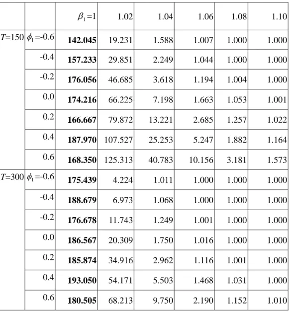
Tables 1, 2, and 3 present the values of ARL, where the varying parameter and its ranges are given in the top row of each table. The baseline case is printed in bold type for each row. The overall in-control ARL can be calculated by

) 1 )( 1 ( 1 /

1 ARL_overall = − −α₁ −α₂ , where α₁ and α₂ denote the probability of committing false alarms for 2

1

T and 2 2

T , respectively. Given α₁=α₂=0.0027, the combination of T and ₁2 T control chart schemes (in (6) and (7), respectively) is ₂2 considered to yield an overall in-control ARL of approximately 185.

Table 1 presents the values of ARL when the true value of β₁ shifts from 1.0 to 1.1, given the same value of φ₁ in each row. The first column denotes the in-control case, in which the values indicate the number of false alarms occurring in 50,000 replications. Almost all of those values printed in bold are less than or close to 185. The ARL values show that the test statistics are sensible to a change in β₁. It is noted that the results are more sensible to a change when the sample size becomes larger, which can be seen by comparing the columns of β₁ =1.02, 1.04, and 1.06 between T=150 and T=300. It also shows that the sensitivity of T is related 2

9

1

φ varies from -0.6 to 0.6, no matter what the sample size is. Here, we only reach a conclusion that the detection of the change in β₁ may depend on the values of φ₁. The pattern for how this differs may depend on more factors, such as the complexity of error function (2) and/or simultaneous shifts in different parameters. To verify this, more simulations should be expected.

Table 2 considers the change of φ₁ in the profile model. We reach similar conclusions about T statistics as with those of Table 1. Again, the ARL value is 2

more sensible to the change for T=150 than that for T=300. However, there lacks a clear pattern with regards to the change of ARL values when comparing the sensitivity due to the left or right deviation from the true value of φ₁. If we look at each row, ARL values are larger for shifts from the left side of the true value than those from the right side for φ₁= -0.6, -0.4, and -0.2. This phenomenon is different for positive values of φ₁, in which ARL values seem more similar on both sides of the true value.

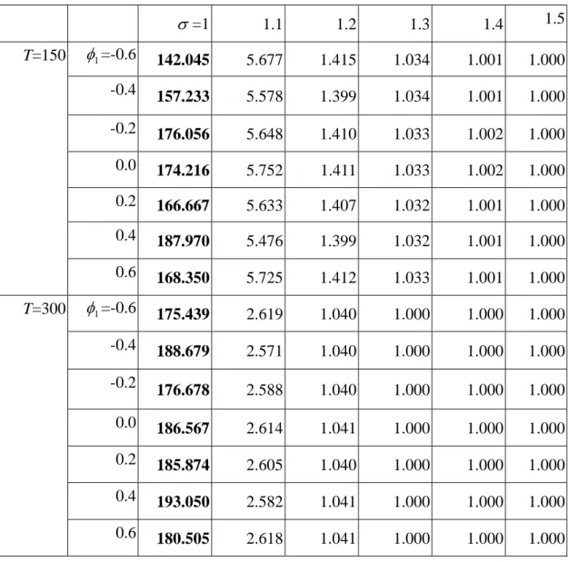
Table 3 examines the deviation of σ from the profile model. Comparing the ARL values row by row yields a similar pattern no matter what the value of φ₁ is. The effect of the sample size appears the same for T=150 and T=300 as shown in Tables 1 and 2. It is noted that both 2

1

T and 2 2

T are able to identify the change in the value of σ , resulting in a significant drop in the ARL values when σ shifts from 1 to 1.1. Nevertheless, 2

2

T is more sensitive to the change than 2 1

T in terms of ARL. While T is a very useful statistic for the change in ₁2 β₁ and φ₁ in Tables 1 and 2, respectively, 2

2

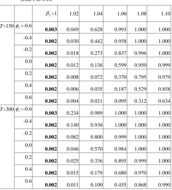
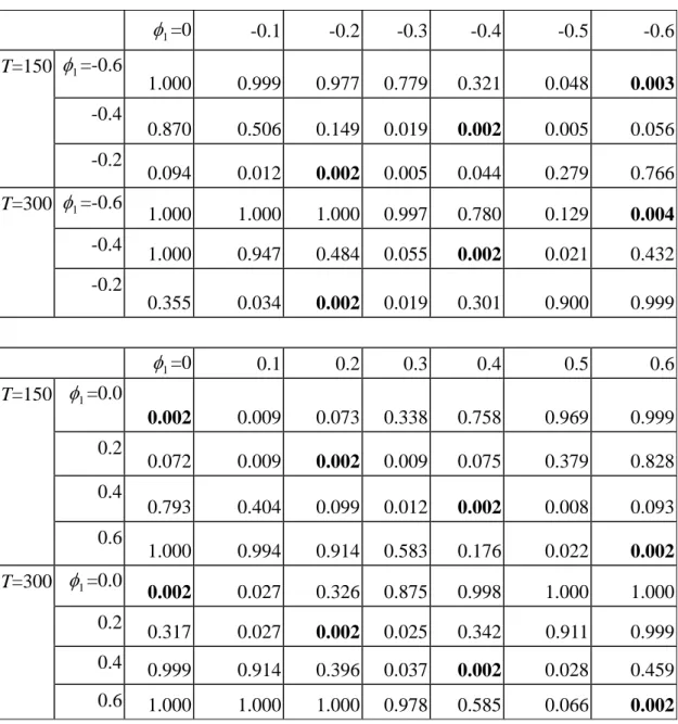
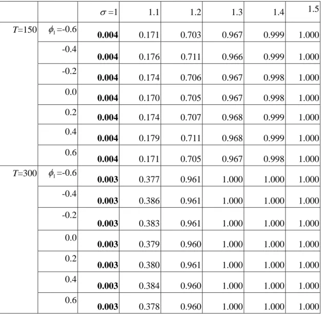
T is not so sensitive to the deviation in β₁ and φ₁. Given α=0.0027, Tables 4 and 5 show the accurate detection rate based on

2 1

T when the values β₁ and φ₁ vary in the same way as the previous tables, respectively. The accurate detection rate is calculated by 1/(out-of-control ARL) given the probability of committing a type I error is 0.0027. The values printed in

10

the bold type are then the estimated false alarm rate. Table 6 presents the accurate detection rate based on 2

2

T when the values of σ change from 1 to 1.1. All these three tables confirm that the proposed statistical approach is sensitive to the change in parameters of concern. It is also noted that the powers of the tests increase as the sample size is larger.

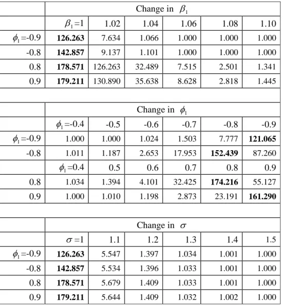
To examine the high correlation problem for an AR(3) errors in models (8) and (9), a new parameter for φ₂ =−0.1 is given to avoid the nonstationarity. Table 7 presents the values of out-of-control ARL with a sample size of 150, where the varying parameter and its ranges are similar to the previous tables, except for the change of φ₁. The performance of using 2

1

T and 2 2

T together on detecting the shift of any one parameter β₁, φ₁, or σ with high correlation errors in the data is similar to those with mild or weak correlation ones.

5. Conclusions

This project proposes approaches to monitoring the profile of the linear regression model with ARMA errors. The first test statistic diagnoses the shift in the coefficients of the linear regression model and the coefficients of the correlated error model. The second test monitors the variance of random errors. The simulation study shows the successful performance in terms of ARL. A real dataset exemplifies the proposed procedure, and graphical analyses enhance the results. This research considers both the Phase I control scheme and Phase II monitoring application, in which the proposed T statistics are quite successful in detecting the abnormal cases. 2

Several issues remain for futher investigation.

According to the simulation, there exists a complex situation on the performance of the proposed test statistics, which depends on the different values of

11

1

φ . We only confirm that this will lead to different conclusions as shown in Tables 1 and 2, which are unable to identify the pattern. This will become more difficult when the error function is more dynamic - for example, the ARMA model with different orders in functions Φ(B) and Θ(B). Furthermore, only one single parameter is allowed to change in the simulation study shown in Tables 1-3. If several parameters simultaneously deviate from that of the candidate profile model, then we expect that the approach will be able to identify the out-of-control situation, but this may require further examinations in order to find out exactly how it happens.

References

Basseville, M., Nikiforov, I.V., 1993. Detection of Abrupt Changes; Theory and Application, Englewood Cliffs, N.J.: Prentice-Hall.

Box, G.E.P., Jenkins, G. M., Reinsel G.C. 2008. Time Series Analysis: Forecasting and Control, 4th ed., New York: John Wiley and Sons.

Brockwell, P.J., Davis, R.A., 2009. Time Series: Theory and Methods, 2nd ed., New York: Springer-Verlag.

Brunato, M, Battiti, R., 2005. Statistical learning theory for location on fingerprinting in wireless LANs. Computer Networks, 47, 825-845

Chatfield, C., 2004. The Analysis of Time Series: an Introduction, Florida: Chapman & Hall.

Chenouri, S., Steiner, S.H., Variyath, A.M., 2009. A multivariate robust control chart for individual observations. Journal of Quality Technology, 41, 259-271.

Durbin, J., Koopman, S.J., 2001. Time Series Analysis by State Space Methods, Oxford: Oxford University Press.

12

methods for online monitoring of linear calibration profiles. International Journal of Production Research, 44, 1927-1942.

Harvey, A.C., 1989. Forecasting, Structural Time Series Models and the Kalman Filter, Cambridge: Cambridge University Press.

Harvey, A.C., Phillips, G.D.A., 1979. Maximum likelihood estimation of regression models with autoregressive-moving average disturbances. Biometrika, 66, 49-58.

Iwashita, T., 1997. Asymptotic null and nonnull distribution of Hotelling's T2-statistic under the elliptical distribution. Journal of Statistical Planning and Inference, 61, 85-104.

Jensen, W.A., Birch, J.B., 2009. Profile monitoring via nonlinear mixed models. Journal of Quality Technology, 41, 18-34.

Jensen, W.A., Birch, J.B., Woodall, W.H. 2008. Monitoring correlation within linear profiles using mixed models. Journal of Quality Technology, 40, 167-183. Kang, L., Albin, S.L., 2000. On-line monitoring when the process yields a linear

profile. Journal of Quality Technology, 32, 418-426.

Kazemzadeh, R.B., Noorossana, R., Amiri, A., 2008. Phase I monitoring of polynomial profiles. Communications in Statistics – Theory and Methods, 37, 1671-1686.

Kim, K., Mahmoud, M.A., Woodall, W.H., 2003. On the monitoring of linear profiles. Journal of Quality Technology, 35, 317-328.

Mahmoud, M.A., Woodall, W.H., 2004. Phase I monitoring of linear profiles with calibration application. Technometrics, 46, 380–391.

Mahmoud, M.A. Parker, P.A., Woodall, W.H., Hawkins, D.M., 2007. A change point method for linear profile data. Quality and Reliability Engineering International, 23, 247-268.

13

Noorossana, R., Amiri, A., Soleimani, P., 2008. On the monitoring of autocorrelated linear profiles. Communications in Statistics - Theory and Methods, 37, 425-442.

Noorossana, R., Eyvazian, M., Amiri, A., Mahmoud, M.A., 2009. Statistical monitoring of multivariate multiple linear regression profiles in phase I with calibration application. Quality and Reliability Engineering International, 26, 291-203.

Pierce, D.A., 1971. Least squares estimation in the regression model with autoregressive-moving average errors. Biometrika, 58, 299-312.

Qiu, P., Zou, C., Wang, Z., 2010. Nonparametric profile monitoring by mixed effects modeling (with discussions). Technometrics, 52, 265-277.

Soleimani, P., Noorossana, R., Amiri, A., 2009. Simple Linear Profiles monitoring in the presence of within profile autocorrelation. Computers & Industrial Engineering, 57, 1015-1021.

Vaghefi, A., Tajbakhsh, S.D., Noorossana, R., 2009. Phase II monitoring of nonlinear profile. Communications in Statistics - Theory and Methods, 38, 1843-1851. Wang, K. and Tsung, F., 2005. Using profile monitoring techniques for a data-rich

environment with huge sample size. Quality and Reliability Engineering International, 21, pp. 677–688.

Williams, J.D., Birch, J.B., Woodall, W.H., Ferry, N.M., 2007. Statistical monitoring of heteroscedastic dose–response profiles from high-throughput screening. Journal of Agricultural, Biological, and Environmental Statistics, 12, 216-235. Williams, J.D., Woodall, W.H., Birch, J.B., 2007. Statistical monitoring of nonlinear

product and process quality profile. Quality and Reliability Engineering International, 23, 925-941.

14

of T2 statistics based on successive differences. Journal of Quality Technology, 38, pp. 217-229.

Woodall, W.H., 2007. Current research in profile monitoring. Revista Producdo, 17, 420-425.

Woodall, W.H., Spitzner, D.J., Montgomery, D.C., Gupta, S., 2004. Using control charts to monitor process and product quality profiles. Journal of Quality Technology, 36, 309-320.

Zou, C., Tsung, F., Wang, Z., 2007. Monitoring general linear profiles using multivariate EWMA schemes. Technometrics, 49, 395-408.

Zou, C., Tsung, F., Wang, Z., 2008. Monitoring profiles based on nonparametric regression models. Technometrics, 50, 512-526.

15

Table 1. Simulated ARL values when β₁ varies from 1 to 1.10 (in-control ARL=185). 1 β =1 1.02 1.04 1.06 1.08 1.10 T=150 φ₁=-0.6 _{142.045 19.231 1.588 1.007 1.000 1.000} -0.4 _{157.233 29.851 2.249 1.044 1.000 1.000} -0.2 _{176.056 46.685 3.618 1.194 1.004 1.000} 0.0 _{174.216 66.225 7.198 1.663 1.053 1.001} 0.2 _{166.667 79.872 13.221 2.685 1.257 1.022} 0.4 _{187.970 107.527 25.253 5.247 1.882 1.164} 0.6 _{168.350 125.313 40.783 10.156 3.181 1.573} T=300 φ₁=-0.6 _{175.439 4.224 1.011 1.000 1.000 1.000} -0.4 _{188.679 6.973 1.068 1.000 1.000 1.000} -0.2 _{176.678 11.743 1.249 1.001 1.000 1.000} 0.0 _{186.567 20.309 1.750 1.016 1.000 1.000} 0.2 _{185.874 34.916 2.962 1.116 1.001 1.000} 0.4 _{193.050 54.171 5.503 1.468 1.031 1.000} 0.6 _{180.505 68.213 9.750 2.190 1.152 1.010}

16

Table 2. Simulated ARL values under the varying values of φ₁ (in-control ARL=185). 1 φ =0 -0.1 -0.2 -0.3 -0.4 -0.5 -0.6 T=150 φ₁=-0.6 1.000 1.001 1.024 1.283 3.089 19.216 145.773 -0.4 _{1.149 1.968 6.539 43.365 177.936 112.867 16.706} -0.2 10.301 60.976 157.729 108.225 20.938 3.544 1.305 T=300 φ₁=-0.6 _{1.000 1.000 1.000 1.003 1.282 7.504 138.122} -0.4 _{1.000 1.056 2.058 17.094 177.305 39.777 2.302} -0.2 _{2.802 27.337} 187.266 44.326 3.294 1.111 1.001 1 φ =0 0.1 0.2 0.3 0.4 0.5 0.6 T=150 φ₁=0.0 174.216 78.125 12.994 2.935 1.317 1.032 1.001 0.2 13.203 76.453 148.810 77.760 12.713 2.621 1.206 0.4 _{1.260 2.460 9.651 60.168 164.474 79.365 10.231} 0.6 _{1.000 1.006 1.094 1.709 5.572 38.580 162.338} T=300 φ1=0.0 186.567 33.201 3.043 1.142 1.002 1.000 1.000 0.2 _{3.128 32.489 168.919 34.626 2.903 1.097 1.001} 0.4 _{1.001 1.094 2.511 24.606 190.840 31.726 2.169} 0.6 1.000 1.000 1.000 1.023 1.706 14.510 171.233

17

Table 3. Simulated ARL values under the shifts of σ from 1 to 1.5 (in-control ARL=185). σ =1 1.1 1.2 1.3 1.4 1.5 T=150 φ1=-0.6 142.045 5.677 1.415 1.034 1.001 1.000 -0.4 _{157.233 5.578 1.399 1.034 1.001 1.000} -0.2 _{176.056 5.648 1.410 1.033 1.002 1.000} 0.0 _{174.216 5.752 1.411 1.033 1.002 1.000} 0.2 _{166.667 5.633 1.407 1.032 1.001 1.000} 0.4 _{187.970 5.476 1.399 1.032 1.001 1.000} 0.6 _{168.350 5.725 1.412 1.033 1.001 1.000} T=300 φ₁=-0.6 _{175.439 2.619 1.040 1.000 1.000 1.000} -0.4 _{188.679 2.571 1.040 1.000 1.000 1.000} -0.2 _{176.678 2.588 1.040 1.000 1.000 1.000} 0.0 _{186.567 2.614 1.041 1.000 1.000 1.000} 0.2 _{185.874 2.605 1.040 1.000 1.000 1.000} 0.4 _{193.050 2.582 1.041 1.000 1.000 1.000} 0.6 _{180.505 2.618 1.041 1.000 1.000 1.000}

18

Table 4. False alarm rate and accurate detection rate based on T when ₁2 β₁ varies from 1 to 1.10. 1 β =1 1.02 1.04 1.06 1.08 1.10 T=150 φ1=-0.6 0.003 0.049 0.628 0.993 1.000 1.000 -0.4 0.002 0.030 0.442 0.958 1.000 1.000 -0.2 0.002 0.018 0.273 0.837 0.996 1.000 0.0 0.002 0.012 0.136 0.599 0.950 0.999 0.2 0.002 0.008 0.072 0.370 0.795 0.979 0.4 0.002 0.006 0.035 0.187 0.529 0.858 0.6 0.002 0.004 0.021 0.095 0.312 0.634 T=300 φ1=-0.6 0.003 0.234 0.989 1.000 1.000 1.000 -0.4 0.002 0.140 0.936 1.000 1.000 1.000 -0.2 0.002 0.082 0.800 0.999 1.000 1.000 0.0 0.002 0.046 0.570 0.984 1.000 1.000 0.2 0.002 0.025 0.336 0.895 0.999 1.000 0.4 0.002 0.015 0.179 0.680 0.970 1.000 0.6 0.002 0.011 0.100 0.455 0.868 0.990

19

Table 5. False alarm rate and accurate detection rate based on T under the varying ₁2 values of φ₁. 1 φ =0 -0.1 -0.2 -0.3 -0.4 -0.5 -0.6 T=150 φ₁=-0.6 1.000 0.999 0.977 0.779 0.321 0.048 0.003 -0.4 0.870 0.506 0.149 0.019 0.002 0.005 0.056 -0.2 0.094 0.012 0.002 0.005 0.044 0.279 0.766 T=300 φ₁=-0.6 1.000 1.000 1.000 0.997 0.780 0.129 0.004 -0.4 1.000 0.947 0.484 0.055 0.002 0.021 0.432 -0.2 0.355 0.034 0.002 0.019 0.301 0.900 0.999 1 φ =0 0.1 0.2 0.3 0.4 0.5 0.6 T=150 φ₁=0.0 0.002 0.009 0.073 0.338 0.758 0.969 0.999 0.2 0.072 0.009 0.002 0.009 0.075 0.379 0.828 0.4 0.793 0.404 0.099 0.012 0.002 0.008 0.093 0.6 1.000 0.994 0.914 0.583 0.176 0.022 0.002 T=300 φ1=0.0 _{0.002 0.027 0.326 0.875 0.998 1.000 1.000} 0.2 0.317 0.027 0.002 0.025 0.342 0.911 0.999 0.4 _{0.999 0.914 0.396 0.037 0.002 0.028 0.459} 0.6 _{1.000 1.000 1.000 0.978 0.585 0.066 0.002}

20

Table 6. False alarm rate and accurate detection rate based on T under the shifts of ₂2 σ from 1 to 1.5. σ =1 1.1 1.2 1.3 1.4 1.5 T=150 φ1=-0.6 _{0.004 0.171 0.703 0.967 0.999 1.000} -0.4 0.004 0.176 0.711 0.966 0.999 1.000 -0.2 0.004 0.174 0.706 0.967 0.998 1.000 0.0 0.004 0.170 0.705 0.967 0.998 1.000 0.2 0.004 0.174 0.707 0.968 0.999 1.000 0.4 0.004 0.179 0.711 0.968 0.999 1.000 0.6 0.004 0.171 0.705 0.967 0.998 1.000 T=300 φ₁=-0.6 0.003 0.377 0.961 1.000 1.000 1.000 -0.4 0.003 0.386 0.961 1.000 1.000 1.000 -0.2 0.003 0.383 0.961 1.000 1.000 1.000 0.0 0.003 0.379 0.960 1.000 1.000 1.000 0.2 0.003 0.380 0.961 1.000 1.000 1.000 0.4 0.003 0.384 0.960 1.000 1.000 1.000 0.6 0.003 0.378 0.960 1.000 1.000 1.000

21

Table 7. Simulated ARL values for high correlation in an AR(3) errors (in-control ARL=185).   Change in β₁   β₁=1 1.02 1.04 1.06 1.08 1.10 1 φ =-0.9 126.263 7.634 1.066 1.000 1.000 1.000 -0.8 142.857 9.137 1.101 1.000 1.000 1.000 0.8 178.571 126.263 32.489 7.515 2.501 1.341 0.9 179.211 130.890 35.638 8.628 2.818 1.445   Change in φ₁   φ₁=-0.4 -0.5 -0.6 -0.7 -0.8 -0.9 1 φ =-0.9 1.000 1.000 1.024 1.503 7.777 121.065 -0.8 1.011 1.187 2.653 17.953 152.439 87.260 1 φ =0.4 0.5 0.6 0.7 0.8 0.9 0.8 1.034 1.394 4.101 32.425 174.216 55.127 0.9 1.000 1.010 1.198 2.873 23.191 161.290   Change in σ   σ=1 1.1 1.2 1.3 1.4 1.5 1 φ =-0.9 126.263 5.547 1.397 1.034 1.001 1.000 -0.8 142.857 5.534 1.396 1.033 1.001 1.000 0.8 178.571 5.679 1.409 1.033 1.001 1.000 0.9 179.211 5.644 1.409 1.032 1.002 1.000

國科會補助計畫衍生研發成果推廣資料表

日期:2012/10/31

國科會補助計畫

計畫名稱: 具相關誤差之線性迴歸模型的剖面曲線監測 計畫主持人: 鄭宗記 計畫編號: 100-2118-M-004-002- 學門領域: 品質管制

無研發成果推廣資料

100 年度專題研究計畫研究成果彙整表

計畫主持人：鄭宗記 計畫編號： 100-2118-M-004-002-計畫名稱：具相關誤差之線性迴歸模型的剖面曲線監測 量化 成果項目 實際已達成 數（被接受 或已發表） 預期總達成 數(含實際已 達成數) 本計畫實 際貢獻百 分比 單位 備 註 （ 質 化 說 明：如 數 個 計 畫 共 同 成 果、成 果 列 為 該 期 刊 之 封 面 故 事 ... 等） 期刊論文 0 1 100% 研究報告/技術報告 0 0 100% 研討會論文 1 1 100% 篇 論文著作 專書 0 0 100% 申請中件數 0 0 100% 專利 已獲得件數 0 0 100% 件 件數 0 0 100% 件 技術移轉 權利金 0 0 100% 千元 碩士生 2 2 100% 博士生 0 0 100% 博士後研究員 0 0 100% 國內 參與計畫人力 （本國籍） 專任助理 0 0 100% 人次 期刊論文 0 0 100% 研究報告/技術報告 0 0 100% 研討會論文 0 0 100% 篇 論文著作 專書 0 0 100% 章/本 申請中件數 0 0 100% 專利 已獲得件數 0 0 100% 件 件數 0 0 100% 件 技術移轉 權利金 0 0 100% 千元 碩士生 0 0 100% 博士生 0 0 100% 博士後研究員 0 0 100% 國外 參與計畫人力 （外國籍） 專任助理 0 0 100% 人次

其他成果

(

無法以量化表達之成 果如辦理學術活動、獲 得獎項、重要國際合 作、研究成果國際影響 力及其他協助產業技 術發展之具體效益事 項等，請以文字敘述填 列。) 無。 成果項目 量化 名稱或內容性質簡述 測驗工具(含質性與量性) 0 課程/模組 0 電腦及網路系統或工具 0 教材 0 舉辦之活動/競賽 0 研討會/工作坊 0 電子報、網站 0 科 教 處 計 畫 加 填 項 目 計畫成果推廣之參與（閱聽）人數 0

國科會補助專題研究計畫成果報告自評表

請就研究內容與原計畫相符程度、達成預期目標情況、研究成果之學術或應用價

值（簡要敘述成果所代表之意義、價值、影響或進一步發展之可能性）

、是否適

合在學術期刊發表或申請專利、主要發現或其他有關價值等，作一綜合評估。

1. 請就研究內容與原計畫相符程度、達成預期目標情況作一綜合評估

■達成目標

□未達成目標（請說明，以 100 字為限）

□實驗失敗

□因故實驗中斷

□其他原因

說明：

2. 研究成果在學術期刊發表或申請專利等情形：

論文：□已發表 ■未發表之文稿 □撰寫中 □無

專利：□已獲得 □申請中 ■無

技轉：□已技轉 □洽談中 ■無

其他：（以 100 字為限）

3. 請依學術成就、技術創新、社會影響等方面，評估研究成果之學術或應用價

值（簡要敘述成果所代表之意義、價值、影響或進一步發展之可能性）（以

500 字為限）

Profile monitoring is a relatively new technique and is becoming popular in the area of quality control, because it is used when the process is characterized by the relationship between a response variable and a set of explanatory variables (i.e., profile) at each time period. This project considers the situation where profiles are modeled parametrically using a multiple linear regression model with random errors following an autoregressive moving-average process. Diagnostic schemes to find out-of-control samples are developed for this purpose. This project conducts a simulation study to examine the performance of the proposed approach based on the average run length criterion. A real example is implemented to illustrate the results, after considering both Phase I and Phase II schemes.