行政院國家科學委員會專題研究計畫 成果報告
Hough 轉換之類神經網路於震測圖型之偵測
計畫類別: 個別型計畫 計畫編號: NSC94-2213-E-009-133- 執行期間: 94 年 08 月 01 日至 95 年 07 月 31 日 執行單位: 國立交通大學資訊科學學系(所) 計畫主持人: 黃國源 報告類型: 精簡報告 報告附件: 出席國際會議研究心得報告及發表論文 處理方式: 本計畫可公開查詢中 華 民 國 95 年 10 月 25 日
行政院國家科學委員會專題研究計畫成果報告
Hough 轉換之類神經網路於震測圖形之偵測
Hough Transform Neural Network for the Detection of Seismic Patterns
計畫編號:NSC 94-2213-E-009-113
執行期限:94 年 8 月 1 日至 95 年 7 月 31 日
主持人:黃國源 交大資訊工程系 [email protected]
一、中文摘要 赫夫轉換類神經網路被應用於單炸點震測 圖形中直接波(直線)與反射波(雙曲線)的 偵測。我們提出以時間軸的座標差定義點 到雙曲線的距離使得參數學習得以實現。 在類神經網路的計算中,一組參數代表一 個圖形,多組參數代表多個圖形,計算點 到多個圖形的距離,當成總誤差,接著利 用梯度下降的最佳化方法,推導出參數修 正的公式,使得點到多個圖形的總誤差為 最小。實驗的結果顯示直線與雙曲線在模 擬的震測圖形中可以被偵測出來。偵測的 結果可以提供作更進一步的解釋。 關鍵詞:赫夫類神經網路,直線偵測,雙 曲線偵測。 AbstractHough transform neural network is adopted to detect line pattern of direct wave and hyperbolic pattern of reflection wave in a one-shot seismogram. We propose the use of time difference from point to hyperbola as the distance. This distance calculation makes the parameter learning feasible. One set of parameters represents one pattern. Many sets of parameters represent many patterns. The neural network can calculate the total error for distances from point to patterns. The parameter learning rule is derived by gradient descent method to minimize the total error. Experimental results show that line and hyperbola can be detected in the simulated data. The detection results can improve the seismic interpretation.
Keywords: Hough transform neural network,
line detection, hyperbolic detection.
二、緣由與目的 近年來類神經網路之研究,在國內外 均極受重視,其應用之領域更是相當的廣 泛。Hough transform (HT) 曾經被應用在 偵測參數圖形[1]-[2],但是記憶體需求與 峰值的偵測是其缺點。即使後來有許多 HT 的 改 良 方 法 , 如 randomized Hough transform 、 rho-theta randomized Hough
transform 、 tree structure Hough
transform 、 generalized Hough transform 等,但仍有同樣的問題。J. Basak 和 A. Das 於 2002、2003 年提出 Hough transform neural network 來 偵 測 直 線 、 圓 與 橢 圓 [3]-[4],可以改善這個問題,但沒有應用 到雙曲線的偵測上。1985 年,Huang 等人 應用 Hough transform 於偵測單點震測圖 中的直接波與反射波[5]。結合以上兩者的 優點,我們提出 Hough transform neural network (HTNN)於雙曲線的偵測,並且應 用在單炸點震測圖形中直接波與反射波之 偵測。
Input one point:
Pattern of p=(ρ1,θ1) Pattern of p’=(ρ1',θ1')
Input next point:
Pattern of p’=(ρ1',θ1') Pattern of p’’=(ρ1'',θ1'') Δp p p'= + Δp p p''= '+
Fig. 1. Illustration of parameter learning. 我們首先給予每個圖形(直線、雙曲線) 一組初始的參數。接著,對於每一個輸入 點,計算點到每一個圖形的距離。然後計
算點對所有圖形的總誤差值,並且利用 gradient descent 的方法來修正每個圖形的 參數,藉以找到使得誤差值最小的參數, 如 Fig. 1 所示。 三、結果與討論 (1) 結果:
(a) Hough Transform Neural Network (HTNN) and Learning Rules
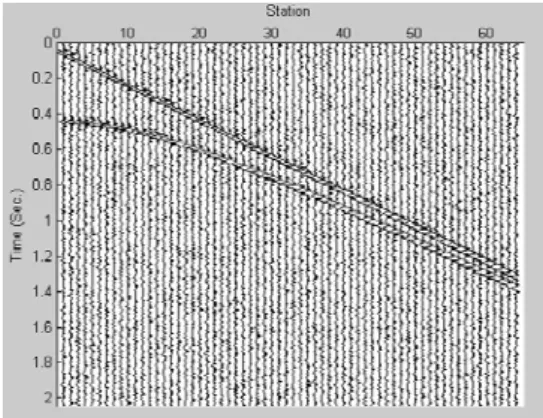
Fig. 2. One-shot seismogram.
Detected patterns Input seis- mogram Hough neural net Pre- processing Detected Parameters
Fig. 3. System for seismic pattern detection.
Fig. 4. Result of thresholding.
Fig. 2 shows the simulated one-shot seismogram with 64 traces and 512 points in each trace. The sampling rate is 0.004
seconds. The size of the input data is 512x64. The proposed detection system is shown in Fig. 3.
The input seismogram in Fig. 1 passes through the thresholding. For seismic data
s( xi,ti ), 1≤xi ≤64 , 1≤ti≤512, we set a
threshold l. If s(xi,ti)≥l, data become the
object points, xi = [xi ti]T, i=1, 2, …, n. Fig.
4 is the thresholding result. Then the data are fed into the network.
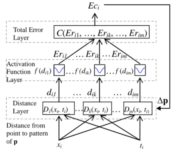
xi ti Eci D1(xi, ti) Dk(xi, ti) Dm(xi, ti) di1 dik dim … … f (di1) f (dik) f (dim) C(Eri1, …, Erik, …, Erim) … … … … Eri1 …Erik… Erim Distance Layer Activation Function Layer Total Error Layer p Δ Distance from point to pattern of p
Fig. 5. Hough transform neural network. The adopted HTNN consists of three layers: distance layer, activation function layer, and the total error layer. The network is shown in Fig. 5. It is an unsupervised network capable of detecting m parameterized objects: lines and hyperbolas, simultaneously.
Input vector xi = [xi ti]T is the ith point
of the image, where i=1, 2, …, n. Input each point xi into distance layer, we calculate the distance dik = Dk(xi) = Dk(xi, ti) from xi to the
kth object (line or hyperbola), k = 1, 2, …, m.
Then, dik passes through the activation
function layer and the output is Erik =1-f(dik),
where f(.) is a Gaussian basis function, i.e.,
) exp( ) ( 2 2 σik ik d d f = −
and Erik is the error or the modified distance
of the ith point to the kth object. Thus, when
ik
d is near zero, Erik is also near zero. In the
last layer, we calculate the total error for
i x ,
∏
≤ ≤ = = = m j ij im ik i i i C C Er Er Er Er Ec 1 1,..., ,..., ) ( ) (ErWhen xi is belonged to one object, then
Erik = 0, and Eci =0.
For a line, Lk(x) = wk,1x + wk,2t + bk = 0,
the parameter vector is pk = [wk,1, wk,2, bk]T.
The distance from point xi to line Lk is Dk(xi)
= | wk,1x + wk,2t + bk| = |Lk(xi)|. From gradient
descent, the derived learning rule for line is
T k T k k =[Δ Δb ] Δp w ( ) T T i ik ik ik ik i d sign d f d Er Ec 1] )[ ( ) ( 1 2 2 ⎟⎠ − x ⎞ ⎜ ⎝ ⎛ ⎟⎟ ⎠ ⎞ ⎜⎜ ⎝ ⎛ − = σ β
Similarly, for a hyperbola with equation 1 2 , 0 2 , 0 = ⎟⎟ ⎠ ⎞ ⎜⎜ ⎝ ⎛ − − ⎟⎟ ⎠ ⎞ ⎜⎜ ⎝ ⎛ − k k k k a x x b t t 0 ) ( 1 ) ( H 0, 2 , 0 + − − = ⎟⎟ ⎠ ⎞ ⎜⎜ ⎝ ⎛ − = k k k k k t t a x x b x
the parameter vector of hyperbola is pk=[ak, bk, x0,k, t0,k]T. the true distance from point to hyperbola is complicated. Here, we consider distance in time from the point (xi,ti) to the
hyperbola Hk(x) = 0 as ) ( H ) ( 1 0, 2 , 0 i k k i k k i k ik t t a x x b d ⎟⎟ + − − = x ⎠ ⎞ ⎜⎜ ⎝ ⎛ − =
We use gradient descent to derive the learning rule for hyperbola,
[
]
( ) ⎥ ⎥ ⎥ ⎥ ⎥ ⎥ ⎥ ⎥ ⎥ ⎥ ⎦ ⎤ ⎢ ⎢ ⎢ ⎢ ⎢ ⎢ ⎢ ⎢ ⎢ ⎢ ⎣ ⎡ + ⎟⎟ ⎠ ⎞ ⎜⎜ ⎝ ⎛ − ⎟⎟ ⎠ ⎞ ⎜⎜ ⎝ ⎛ − ⎟⎟ ⎠ ⎞ ⎜⎜ ⎝ ⎛ − + ⎟⎟ ⎠ ⎞ ⎜⎜ ⎝ ⎛ − + ⎟⎟ ⎠ ⎞ ⎜⎜ ⎝ ⎛ − ⎟⎟ ⎠ ⎞ ⎜⎜ ⎝ ⎛ − ⎟⎟ ⎠ ⎞ ⎜⎜ ⎝ ⎛ − ⋅ − ⎟⎟ ⎠ ⎞ ⎜⎜ ⎝ ⎛ ⎟ ⎠ ⎞ ⎜ ⎝ ⎛ − = Δ Δ Δ Δ = Δ 1 1 1 1 ) ( ) ( 1 2 2 , 0 , 0 2 , 0 2 , 0 2 , 0 2 , 0 , 0 k k i k k i k k k k i k k i k k i k k ik ik ik ik i T k k k k k a x x a x x a b a x x a x x a x x a b d sign d f Er d Ec t x b a σ β p (b) Experimental ResultsThe HTNN is applied to the simulated one-shot seismogram. For flat reflecting layer, we can get x0=0, so three parameters must be detected for hyperbola.
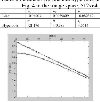
The image space of simulated one-shot seismogram in Fig. 2 is 512x64. After preprocessing, the input data in Fig. 4 have 252 object points. Table I shows the detected parameters of line and hyperbola in
the image space. The experimental results are shown in Fig. 6-8. Fig. 6 shows the result of detection of direct wave and reflection wave in the x-t space. Fig. 7 shows the error versus iteration number, where the dotted line represents the 12 iterations when the iteration number from stage one to stage two. We combine the detection results to the original seismogram and shown in Fig. 8. The result of experiment is quite successful.
Table I. Parameters of line and hyperbola in Fig. 4 in the image space, 512x64.
w1 w2 b
Line -0.040031 0.0079809 -0.082842
a b t0
Hyperbola -21.176 -10.383 4.5614
Fig. 6. Detection result: direct wave and reflection wave.
Fig. 8. Detected line and hyperbola on one-shot simulated seismogram.
(2) 討論:
HTNN is adopted to detect line pattern of direct wave and hyperbola pattern of reflection wave in a one-shot seismogram. The parameter learning rule is derived by gradient descent method to minimize the error. We calculate the distance from point to line. Also we define the vertical time difference as the distance from point to hyperbola that makes the learning feasible. In experiments, we get fast convergence in simulated data because three parameters are considered in the hyperbolic detection. The detection results can improve seismic interpretation.
The result of preprocessing is quite critical for the input-output relation. More wavelet, envelope, and deconvolution processing may be needed in the preprocessing to improve the detection result.
四、成果自評
研究內容與原計畫相符程度: 100% 達成預期目標情況: 100%
研究成果的學術或應用價值: 建立 Hough
transform neural network 於 震 測
one-shot seismogram 直接波與反射波 參數之偵測及圖形之還原,可幫助探油 的震測解釋 是否適合在學術期刊發表: 是 主要發現或其他有關價值: 可用於其他影 像圖形之偵測。 五、參考文獻
[1] Hough, P.V.C., Method and means for recognizing complex patterns: U.S. Patent 3069654, 1962.
[2] Duda, R.O., and Hart, P.E., Use of the Hough transform to detect lines and curves in pictures: Communications of the ACM, 15, 11-15, 1972
[3] Basak, J. and Das, A., Hough transform networks: Learning conoidal structures in a connectionist framework: IEEE Transactions on Neural Networks, 13, no. 2, 381-392, 2002.
[4] Basak, J. and Das, A., Hough transform network: A Class of networks for identifying parametric structures: Neurocomputing, 51, 125-145, 2003.
[5] Huang, K.Y., Fu, K.S., Sheen, T.H., and Cheng, S.W., Image processing of seismograms: (A) Hough transformation for the detection of seismic patterns. (B) Thinning processing in the seismogram: Pattern Recognition, 18, no.6, 429-440, 1985.
[6] Dempsey, G.L. and McVey, E.S., A Hough transform system based on neural networks: IEEE Transactions on Industrial electronics, 39, 522-528, 1992.
[7] Dobrin, M. B., Introduction to geophysical prospecting: 3rd ed., McGraw-Hill, 1976
[8] Slotnick, M. M., Lessons in seismic computing: The Society of Exploration Geophysicists, 1959.
[9] Yilmaz, O., Seismic data processing: Society of Exploration Geophysicists, 1987.