Gbps高速渦輪碼之設計與實現

(1)

國立交通大學

電子工程學系電子研究所碩士班

碩士論文

Gbps 高速渦輪碼之設計與實現

Design and Implementation of Gbps Turbo Decoders

學生：賴名威

指導教授：李鎮宜教授

(2)

Gbps 高速渦輪碼之設計與實現

Design and Implementation of Gbps Turbo Decoders

研究生：賴名威 Student：Ming-Wei Lai

指導教授：李鎮宜 Advisor：Chen-Yi Lee

國立交通大學

電子工程學系電子研究所碩士班

碩士論文

A Thesis

Submitted to Department of Electronics Engineering & Institute of Electronics College of Electrical and Computer Engineering

National Chiao Tung University in Partial Fulfillment of the Requirements

for the Degree of Master of Science

in

Electronics Engineering July 2007

Hsinchu, Taiwan, Republic of China

(3)

Gbps 高速渦輪碼之設計與實現

學生：賴名威指導教授：李鎮宜教授

國立交通大學

電子工程學系電子研究所碩士班

摘要

自九零年代初渦輪碼被發現以來，由於出色的錯誤更正能力一直以來廣泛的引起研究者的注意，在近期寬頻無線通訊以及第四代行動通訊等協定中，對於高速渦輪碼的資料流量的要求，也分別訂定了每秒 70Mb 以及每秒 20Mb 到 100Mb 的高速傳輸量，因此，對於高速渦輪碼的需求也與日俱增。而在渦輪碼的解碼中，由於尋找最大事後機率的解碼方式中，含有遞迴式的計算方式，也因此造成了在渦輪碼的解碼中，產生了很可觀的時間延遲。在這篇論文當中，針對高速的渦輪碼解碼，我們提出了一個完整的解決方案，其中，包含一個資料讀寫平順無誤的打散器設計，一個多級高階的渦輪解碼器，以及提出ㄧ種能夠運用在兩個維度的平行解碼器架構，由於這些因素，使得我們在本論文中所提出的設計，與現今科技之水準比較下，達到最高的能源效率以及每秒的資料解碼量，達到最高的水準。

(4)

Design and Implementation for Gbps Turbo Decoders

Student : Ming-Wei Lai Advisor : Dr. Chen-Yi Lee

Institute of Electronics Engineering

National Chiao Tung University

ABSTRACT

Turbo codes have received a lot of interest since 90’s because of their excellent performance. To apply turbo codes in high-speed digital communications, such as in broadband wireless access based on the IEEE 802.16 standard supporting data rates of up to 70 Mb/s, and in fourth generation cellular systems, which are expected to provide a data rate from 20 to 100 Mb/s for high mobility, high throughput of turbo codes is a critical issue. The recursive computations in the MAP-based decoding of turbo codes usually introduce a significant amount of decoding delay. In this thesis, we present a total solution for a high throughput application, including a contention-free interleaver design, a high radix turbo decoder design, and the two-dimension parallel decoding architecture. The chip proposed in this thesis is the most power efficient and the fastest design in the state of the art.

(5)

誌謝

忙碌而充實的研究生生活，隨著口試的結束也悄悄地接近了尾聲。在這二年的研究生涯中，首先要感謝指導教授李鎮宜教授在這段時間對我的指導，並且提供一個良好的研環境讓我能夠專注於學業與研究。此外，還要感謝 Si2 實驗室以及 Ocean Group 所有的成員，在這段時間給了我非常多的協助與討論，使得我的研究得以順利的完成。其中，特別要感謝張錫嘉教授、林建青學長、陳志龍學長以及翁政吉學長給予我非常多的協助與指導，並且在相互的討論中，給予了我非常多的構想與啟發，使得這些研究能夠順利的完成。最後，感謝我的父母一路上對我的支持與協助，沒有你們也就沒有今天的我。

(6)

List of Figures

FIG.1.1THE BLOCK DIAGRAM OF DIGITAL COMMUNICATION SYSTEM...2

FIG.2.1TURBO ENCODER FOR 3GPP2 STANDARD...5

FIG.2.2TRELLIS TERMINATION...5

FIG.2.3TURBO DECODING FLOWCHART...7

FIG.2.4TRELLIS DIAGRAM OF TURBO CODE IN 3GPP2 STANDARD...9

FIG.2.5THE PROCESS DIAGRAM OF SLIDING WINDOW APPROACH IN THE FORWARD DIRECTION.17 FIG.2.6THE PROCESS DIAGRAM OF SLIDING WINDOW APPROACH IN THE BACKWARD DIRECTION ...18

FIG.2.7THE ENCODER PROCESS OF TAIL-BITING CONVOLUTIONAL CODE...20

FIG.3.1BLOCK DIAGRAM OF PROPOSED TURBO DECODER...22

FIG.3.2BLOCK DIAGRAM OF PROPOSED TURBO DECODER...23

FIG.3.3EXAMPLE OF A CONTENTION-FREE PERMUTATION...24

FIG.3.4AN EXAMPLE OF IBP INTERLEAVER WITH FOUR SUB-BLOCKS...25

FIG.3.5A4X4 BUTTERFLY NETWORK FOR IBP INTERLEAVER...26

FIG.3.6RETIMING PROCEDURE OF A RADIX 2X2ACS UNIT...28

FIG.3.7A RETIMED RADIX 2X2ACS UNIT...28

FIG.3.8THE CIRCUIT FOR LOG-LIKELIHOOD CALCULATION...29

FIG.3.9FER PERFORMANCE COMPARED WITH 3GPP TURBO CODE...30

FIG.3.10BER PERFORMANCE COMPARED WITH 3GPP TURBO CODE...31

FIG.3.11MICRO PHOTO OF PROPOSED TURBO DECODER CHIP...33

FIG.4.1A CYCLE-BASED DECODING PROCEDURE...36

(10)

FIG.4.3DECODING SCHEDULE OF A SUB-CODEWORD...37

FIG.4.4DECODING SCHEDULE OF PREVIOUS DESIGN...37

FIG.4.5DECODING SCHEDULE WITH TWO CODEWORDS...38

FIG.4.6RADIX 16 AND RADIX 4X4TRELLIS DIAGRAM...40

FIG.4.7CIRCUIT DIAGRAMS OF TWO STRUCTURES...40

FIG.4.8THE MEMORY UNIT...41

FIG.4.9A CRITICAL PATH COMPARISON...42

FIG.4.10THE ARCHITECTURE TRANSFORMATION...43

FIG.4.11MULTIPLE BLOCK LENGTHS SUPPORT...44

FIG.4.12POWER ISOLATION OF DLL ...45

FIG.4.13CHIP LAYOUT VIEW...45

FIG.5.1THE ARCHITECTURE OF 1GBPS TURBO DECODER...49

FIG.5.2DECODING PROCEDURE OF SLIDING WINDOW APPROACH...49

FIG.5.3A SECTIONALIZED METHOD...50

FIG.5.4DIFFERENT SIZES OF THE SECTIONALIZED METHOD...50

FIG.5.5COMPARISON OF DIFFERENT STRUCTURES...51

FIG.5.6A TWO-DIMENSION PARALLEL METHOD...52

FIG.5.7A INTRA-CODEWORD PARALLEL ARCHITECTURE...53

FIG.5.8DATA HAZARDS...54

FIG.5.9A PROPER DECODING ORDER FOR DATA HAZARDS...54

FIG.5.1064T PERFORMANCE...55

(11)

FIG.5.168T EXTEND TO 16T ...58

FIG.5.174T EXTEND TO 8T,12T, AND 16T ...59

FIG.5.18THE ORIGINAL DECODING SCHEDULE...60

FIG.5.19 EXAMPLE OF THE NEW 8T AND 16T DECODING SCHEDULE...60

(12)

List of Tables

TABLE 1.1 COMPARISON OF TURBO CODE AND LDPC ... 2

TABLE 3.1 TURBO DECODER SPECIFICATION ... 32

TABLE 3.2 COMPARISON WITH OTHER TURBO DECODER... 34

TABLE 4.1 COMPARISON BETWEEN TWO VERSIONS ... 42

TABLE 4.2 SUMMARY OF THE PROPOSED 1GBPS TURBO DECODER... 46

TABLE 5.1 HARDWARE COMPARISON OF TWO-DIMENSION PARALLEL ARCHITECTURE ... 62

TABLE 5.2 HARDWARE COMPARISON OF INTRA-CODEWORD PARALLEL ARCHITECTURE ... 62

(13)

Chapter 1 Introduction

1.1 Motivation

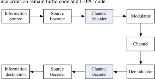
A communication system conveys a information source to a destination through a channel. Fig. 1.1 shows a fundamental block diagram of traditional digital communication system. Generally, the system can be divided into transmitter and receiver via a channel. The main task of transmitter, including source encoder, channel encoder and modulator, is to transform the information into a form that can withstand the effect of noise over the transmission media. And the receiver will reverse the signal transformation by demodulator, channel decoder and source decoder. Since the channel impairments such as noise, interference and distortion may cause the error in the received signal, the channel encoder is incorporated in the system to add certain structural redundancy to the source codeword to minimize the transmission errors. Although these redundant bits may lower data transmission rate, the channel coding eliminate the effects of noise disturbances and thus improve the performance, compared with an uncoded system.

With high coding gain provided by channel codes, the high performance channel codes are widely used in some circumstances, such as low power transmission, high order modulation, and complex channel conditions, in the recent decades. In channel codes, there are three codes that provide marvelously high performance: block turbo code, convolutional turbo code, briefly called turbo code, and low density parity check code. The block turbo code is hard to implement due to the irregular Trellis structure. Therefore, the candidates for the

(14)

high performance criterion remain turbo code and LDPC code.

Fig. 1.1 The block diagram of digital communication system

The comparison of turbo code and LDPC are listed in Table 1.1. From the point of view with block length bigger than 10000, the performance of LDPC would be better than turbo code due to the property of component codes. With block length smaller than 10000, the performance of turbo code would be better due to the girth problem of LDPC. The Parallelism of LDPC is easier for implementation than turbo code. Most important of all, the routing problem of LDPC is getting serious as the throughput demand growing. Meanwhile, the advanced process for high speed implementation aggravates the routing congestion problem of LDPC. Apparently, for a high speed application, the turbo codes would be more suitable and area-efficient if we can increase the throughput of the turbo codes.

Table 1.1 Comparison of Turbo code and LDPC

LDPC Code Turbo Code

>10000 Better Good

Performance

(Block length) _<10000 _Good _Better

Throughput (Parallelism) Better Medium

Efficiency Medium Medium

(15)

In this thesis, our work is motivated to design a high performance and high-throughput turbo decoder. We attempt to achieve the target from two aspects: First one is to speed up the decoding processing elements used in the whole turbo decoder by high radix structures and perfect utilization of hardware. Second, we employ a well-designed interleaver fit for parallel decoding architectures to reduce the latency caused by the interleaver and propose a practical hardware architecture for the whole turbo decoder. Finally, we will propose a new point of view of parallel decoding for MAP-based turbo decoder with the modest hardware cost.

1.2 Thesis Organization

This thesis consists of 7 chapters. In chapter 2, we’ll focus on interpreting turbo coding and decoding algorithm and its relative techniques. Chapter 3 presents a total solution of a high speed turbo decoder with a parallel architecture, including the design of a contention-free interleaver, a high radix turbo decoder, and some techniques applied on our design. Chapter 4 explains how we improve the utilization of the previous chip. A Modified interleaver control for multiple block lengths support will be introduced. In chapter 5, we present the two architectures. A two-dimension parallel architecture will be proposed. Meanwhile, a simplified intra-codeword parallel architecture and the relative issues will be discussed. Finally, conclusion and future work are made in chapter 6.

(16)

Chapter 2 Turbo Code

The parallel concatenated convolutional code (PCCC), named turbo code, was first proposed by C. Berrou, A. Glavieux, and P. Thitimajshima in 1993[1]. It has been proved to have a performance close to Shannon limit with simple constituent codes concatenated by an interleaver. This new technique is now adopted in 3GPP, 3GPP2 and WiMAX standards due to its excellent error correction ability. In this chapter, we’ll describe the principle of both turbo encoding and turbo decoding methods. The sliding-window approach and the tail-biting coding structure will also be interpreted here.

2.1 Principle of Turbo code

2.1.1 Turbo Encoding

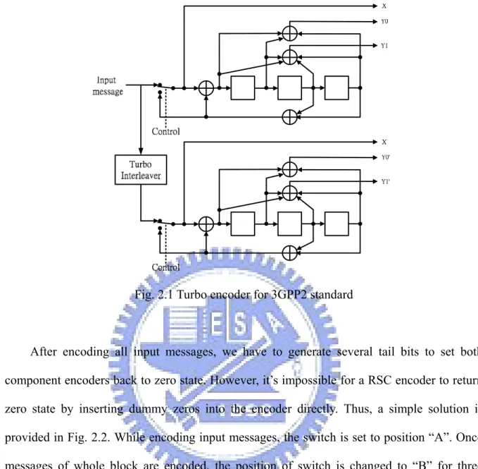
The turbo encoder is composed of two recursive systematic convolutional (RSC) encoders, which are connected in parallel but separated by a turbo interleaver. The two RSC encoders are also called constituent codes of the turbo code. The block diagram of the turbo encoder is illustrated in Fig. 2.1. Note that the same input data are encoded by each RSC encoder but in different order. In 3GPP2 standard, each input bit is encoded as one systematic bit and two parity-check bits for each RSC encoder. Thus, the code rate of each component encoder is 1/3. In order to increase the code rate of turbo code, the systematic bits of the second RSC encoder are not transmitted. Therefore, the output encoded sequence should be {X, Y0, Y1, Y0’, Y1’}, and the overall code rate is 1/5.

(17)

Fig. 2.1 Turbo encoder for 3GPP2 standard

After encoding all input messages, we have to generate several tail bits to set both component encoders back to zero state. However, it’s impossible for a RSC encoder to return zero state by inserting dummy zeros into the encoder directly. Thus, a simple solution is provided in Fig. 2.2. While encoding input messages, the switch is set to position “A”. Once messages of whole block are encoded, the position of switch is changed to “B” for three additional cycles. This will force all registers to zeros and thus back to zero state.

Systematic bit Parity-check bit Input message A B

(18)

2.1.2 Turbo Interleaver

The interleaver plays a very important role in turbo encoder. First of all, a proper coding gain can be achieved with small memory RSC encoders since the interleaver scramble a long block message. Besides, the interleaver de-correlates the input of two RSC encoders so that iterative decoding algorithm can be applied between two component decoders. Theoretically, the block size of interleaver is one of the major factors to lower the upper bound on bit error probability of the turbo code system. The performance upper-bound of turbo code corresponding to a uniform random interleaver has been evaluated in [9]. The result shows that the bit-error-probability upper bound of turbo code is approximately proportional to 1/N, where N is the block size of turbo interleaver. The factor “1/N” is also called the interleaver gain.

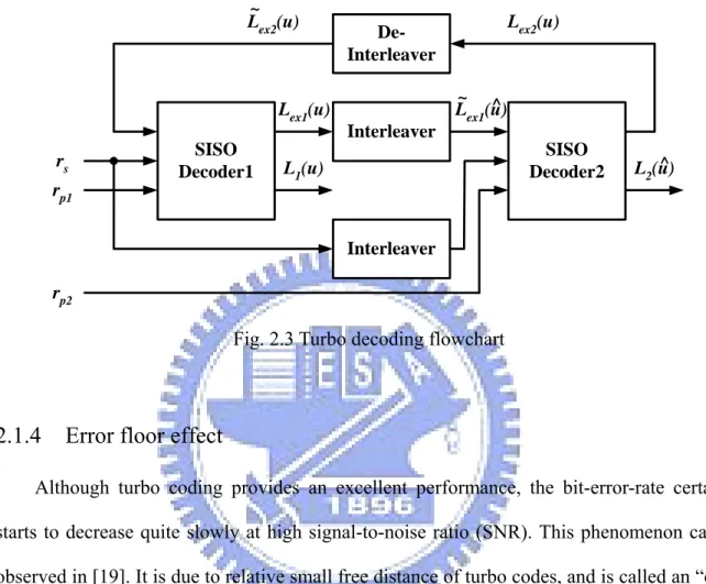
2.1.3 Turbo Decoding

A general idea for iterative turbo decoding is illustrated in Fig. 2.3, where rs is the

received systematic information, rp1 is the received parity information generated by the first

RSC encoder, and rp2 is the received parity information generated by the second RSC encoder.

The iterative turbo decoding consists of two constituent decoders, which are soft-in/soft-out (SISO) decoders concatenated serially via one interleaver and one de-interleaver. An additional interleaver is used to interleave the input systematic information and then provides the interleaved data to the second SISO decoder. Two component decoders can be implemented based on either soft-output Viterbi algorithm (SOVA) [21] or maximum a

posteriori probability (MAP) algorithm [2], which will be discussed particularly in the next

section. During iterative decoding process, each constituent decoder delivers the extrinsic information Lex(u) which is taken as a priori information for the other constituent decoder.

(19)

better coding gain is expected. However, the correlation between two SISO decoders is also raised up. Therefore, there is no significant performance improvement if the number of iterations reaches a threshold.

SISO Decoder1 SISO Decoder2 Interleaver De-Interleaver Interleaver L_ex1(u) L₁(u) r_s r_p1 r_p2 L~_ex1(u)^ L₂(u)^ L~_ex2(u) L_ex2(u)

Fig. 2.3 Turbo decoding flowchart

2.1.4 Error floor effect

Although turbo coding provides an excellent performance, the bit-error-rate certainly starts to decrease quite slowly at high signal-to-noise ratio (SNR). This phenomenon can be observed in [19]. It is due to relative small free distance of turbo codes, and is called an “error floor” [22]. Consider the relation of the minimum free distance and the bit error probability in turbo coding, which can be expressed by

0 2 b b free E P Q d R N ⎛ ⎞ ∝ ⎜⎜ ⎝ ⎠⎟⎟ (2. 1) where dfree is the minimum free distance and Eb/N0 is the SNR. At low SNR, the major part of

errors can be corrected by iterative decoding since systematic information and parity information can be regarded as highly independent events. However, as the channel provides a reliable transmission, the dependency of the systematic and parity information grows up and the interleaver does little contribution on iterative decoding. Thus, the error correction ability

(20)

is limited on the weak constituent code only. To overcome this issue, we can increase the interleaver size to lower the position of the error floor or concatenate a block code, e.g. BCH code, as an outer code to remove the left error bits. For more details, please refer to [9] [23].

2.2 Decoding Algorithms for Turbo Code

It has been proved that the MAP algorithm is the optimal decoding method for turbo code while comparing with SOVA [10]. Unlike Viterbi algorithm which utilizes maximum likelihood (ML) algorithm to find the codewords with minimum error probability, the MAP algorithm minimizes the symbol (or bit) error probability. In this section, we’ll focus on introducing the turbo decoding methods based on MAP algorithm [2][3]. Although SOVA is also one of the commonly used techniques for turbo decoding, we’ll skip it since it’s not adopted in our proposed design. To understand more detail about SOVA, please refer to [21]. And some comparisons of MAP algorithm and SOVA applied in turbo code system are shown in [10].

2.2.1 The MAP algorithm

The main idea of MAP algorithm is to compute the log-likelihood ratio (LLR) of the transmitted information bit uk conditioned on the received information rk for 1≦k≦N, where

N is the block length of encoded message.

( 1| ˆ ( ) ( | ) log ( 1| k k k k P u L u L u P u ) ) = + = = = − r r r (2. 2)

Here r is the vector of received soft values, and can be represented as [r1,r2, …, rn] where n is

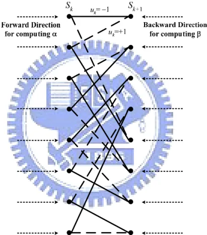
the number of output bits for each encoded bit in the constituent code. Let’s consider the trellis diagram of turbo code in 3GPP2 standard, which is shown in Fig. 2.4 as an example. Note that the solid lines represent the transitions corresponding to an information bit uk of -1,

(21)

Then, the equation can be further expressed as ( 1| ) ˆ ( ) log log ( 1| ) k k -1 k u =+1 k k k k u =-1 P(s ,s , ) P u L u P u P(s ,s , ) = + = = = − k -1 k

∑

r r r r . (2. 3)

where the numerator and denominator are the sum of joint probabilities for all existing transitions from state sk-1 to state sk that corresponding to an information bit uk of +1 and -1

respectively.

Fig. 2.4 Trellis diagram of turbo code in 3GPP2 standard

Assume the encoded data is transmitted through the discrete memoryless channel (DMC), and then the term P(sk-1,sk,r) can be decomposed as three terms:

1 1 1 1 1 1 ( ) ( , ) ( ) ( , , ) ( , ) ( , | ) ( | k k k k k k k k k k j k k k k j k k s s s s P s s P s r P s s P r s eα− − eγ − eβ − = − < ⋅ − ⋅ > = ⋅ ⋅ ) r r . (2. 4) Here _eαk−1(sk−1) is the joint probability of state s

(22)

of the block up to time index “k-1”. Similarly, _eβk( )sk is that of state s

k and received symbols

rj from the end of block back to time index “k”. By shifting the value “k”, it can be perceived

that α is the forward recursion of the MAP algorithm, and can be formulated as

1 1 1 ( ) ( , ) ( ) k k k k k k k k s s s s eα eγ − eα− − =

∑

⋅ s−1 . (2. 5)

The same as above, the backward recursion β can be formulated as

1( 1) ( 1, ) ( ) k k k k k k k k s s s s s eβ− − =

∑

eγ − ⋅eβ . (2. 6)

Note that since the trellis of turbo code diverges from state zero and converges to state zero, the initial condition of the forward recursion and backward recursion should be set as

0 0 0 0 ( ) 0 ( ) 1, for 0 0, otherwise s s e e α α ⎧ = s = ⎨ = ⎩ (2. 7) and ( ) ( ) 1, for 0 0, otherwise N N N N s N s e e β β ⎧ = s = ⎨ = ⎩ (2. 8) For any existing transitions from sk-1 to sk, the branch transition probability eγk(sk−1, )sk can be

further decomposed as 1 ( , ) 1 1 1 ( , | ) ( | ) ( | , ) ( ) ( | ) k sk sk k k k k k k k k k k k e P s s P s s P s s P u P u γ − − − − = = ⋅ = ⋅ r r r . (2. 9)

Here, the term “P(uk)” is well-known as a priori probability. According to the definition of

LLR, which is ( ( ) log ( 1 k k k P u L u P u 1) ) = + = = − , (2. 10)

(23)

( ) ( ) ( ) / 2 ( ) / 2 ( ) ( ) / 2 ( 1) 1 1 . k k k k k k k k L u k L u L u L u u L u L u u k e P u e e e e A e ± ± − ⋅ − ⋅ = ± = + = ⋅ + = ⋅ (2. 11)

where the term Ak is equal for all transitions at the same time index, and thus will cancel out

in (2. 3). On the other hand, the value of P(rk|uk) is dependent on channel characteristic. For

an additive white Gaussian noise (AWGN) channel, the LLR of rk conditioned on uk can be

expressed as 2 , , 1 0 1 2 , , 1 0 1 , , 1 ( | 1) ( ) log ( | 1) exp( ( ) ) log exp( ( ) ) k k k k k k k k n s k v k v v u n s k v k v v u n c k v k v v P u L u P u E r x N E r x N L r x = =+ = =− = = + = = − − − = − − = ⋅ ⋅

∏

∑

r r r (2. 12)

where Lc=4Es/N0 and is called the channel reliability. Here, xk,v is the v-th transmitted symbol

while encoding uk. For systematic codes, xk,1 is equal to uk. Now we can obtain the value of

P(rk|uk) by using the technique in (2. 11) but substitute L(uk) with L(rk|uk).

,1 , , 2 1 1 ( | ) exp( ) 2 2 n k k k c k k c k v k v v P u B L r u L r x = = ⋅ +

∑

r (2. 13)

For the same reason in (2. 11), Bk will also cancel out in (2. 3). Combining (2. 11) and (2. 13),

the γk in (2. 9) can be reduced to

1 ( , ) ,1 , , 2 1 exp ( ( )) 2 k k k n s s k k c k k k c k v k v v eγ − A B L r L u u L r x = ⎛ ⎛ ⎞⎞ = ⋅ ⋅ _⎜ _⎜ + ⋅ + _⎟_⎟ ⎝ ⎠ ⎝

∑

⎠. (2. 14) Substituting (2. 5), (2. 6), (2. 14) into (2. 4), we can derive the a posteriori LLR in the form of

(24)

1 1 1 1 1 1 1 1 ( ) ( , ) ( ) ( , ) 1 ( ) ( , ) ( ) ( , ) 1 ,1 ˆ ( ) log ( ) ( ) k k k k k k k k k k k k k k k k k k k k s s s s s s u k s s s s s s u c k k ex k e e e L u e e e L r L u L u α γ β α γ β − − − − − − − − =+ =− ⋅ ⋅ = ⋅ ⋅ = + +

∑

(2. 15) where , , 1 1 2 1 , , 1 1 2 1 1 2 ( ) ( ) ( , ) 1 1 2 ( ) ( ) ( , ) 1 k ( ) log n c k v k v k k v k k k k k n c k v k v k k v k k k k L r x s s s s u ex k L r x s s s s e e e L u e e e α β α β − − = − − − = − =+ ∑ ⋅ ⋅ = ∑ ⋅ ⋅

∑

. (2. 16) coder

nt decoder, and great performance improvement in iterative AP decoding can be achieved.

2.2.

his problem can be solved by Log-MAP algorithm [24]. It employs the Jacobian algorithm

u =−

The term Lex(uk) is called extrinsic information since it’s a function of the redundant

information that comes from the en . It removes the information about the systematic input and a priori information fromL u( )ˆ_k . Therefore, this term is useful to estimate a priori probability for the next compone

M

2 The Log-MAP algorithm

It can be figured out easily that Max-Log-MAP algorithm is a sub-optimal solution for turbo decoding since an approximation of (2. 21) is used to reduce the complexity of MAP algorithm. T 1 2 1 2 1 2 1 2 1 2 max( , )δ δ f_c(δ δ ), = + − where f

log(eδ +eδ ) max( , ) log(1= δ δ + +e− −δ δ )

(2. 17) has been proved that (2. 21) can be computed exactly by a recursive operation of (2. 25) [10].

(25)

1 1 2 1 2 log( ) log( ), max(log , ) ( log ) max( , ) ( ) n n n n c n n c n e e e e e e e e f f δ δ δ δ δ δ δ δ δ δ δ δ δ δ − + + + = ∆ + ∆ = + + + = = ∆ + ∆ − = + − (2. 18)

Substituting (2. 18) and (2. 19) into (2. 25), the forward and backward recursions can be represented as

(

)

1, 1 1 1 ( ) max* ( ) ( , ) k k k k k k k k k s u s s s α α γ − − − − = + s (2. 19) and

(

)

1( 1) max*_, ( ) ( 1, ) k k k k k k k k k s u s s s β ₋ ₋ = β +γ ₋ s , (2. 20)

where the max*(.) operation is defined as

1 2

1 2 1 2

max*( , ) max( , ) log(1δ δ = δ δ + +e− −δ δ ). (2. 21) Finally, L u( )ˆ_k can be obtained by

(

)

(

)

1 1 1 1 1 ( , ) 1 1 1 1 ( , ) 1 ˆ ( ) max * ( ) ( , ) ( ) max * ( ) ( , ) ( ) . k k k k k k k k k k k k k s s u k k k k k k k s s u L u s s s s s s s s α γ β α γ β − − − − − =+ − − − =− = + + − + + k c c 1 2 (2. 22)

The performance of Log-MAP algorithm is identical to that of MAP algorithm. However, the complexity is also increased compared with Max-Log-MAP algorithm since computing

f (.) still involves complicated exponentiations and multiplications. Thus, the values of f (.)

are usually stored in a pre-computed table and Log-MAP algorithm can be implemented by table look-up. It has been found that excellent performance can be obtained with 8 stored values and |δ -δ | ranging between 0 and 5, and no improvement is achieved with a finer

representation [10].

2.2.3 The Max-Log-MAP algorithm

(26)

multiplications. These are quite complex for hardware realization. Thus, an approximation of MAP algorithm termed Max-Log-MAP algorithm [24] was derived for simple implementation of MAP decoders. Instead of calculating _eγk, _eαk, and _eβk directly, all computations are

done in logarithm domain. Here we define γk, αk, and βk as transition metric, forward path

metric and backward path metric respectively. γk can be formulated as

1 1

( , ) log ( , |

k sk sk P sk k sk )

γ ₋ = r ₋ . (2. 23)

Similarly, referring to (2. 4), αk and βk can be expressed as

( ) log ( , ) k sk P sk j k α = r_< (2. 24) and 1( 1) log ( | k sk P j k sk) β ₋ ₋ = r_> (2. 25)

respectively. After substituting (2. 17), (2. 18), and (2. 19), in (2. 15) can be re-written as ˆ ( )_k L u

(

)

(

)

1 1 1 1 1 ( , ) 1 1 1 1 ( , ) 1 exp ( ) ( , ) ( ) ˆ ( ) log exp ( ) ( , ) ( ) k k k k k k k k k k k k k s s u k k k k k k k k s s u s s s s L u s s s s α γ β α γ β − − − − − =+ − − − =− + + = + +

∑

. (2. 26)

By utilizing the approximation of

1 2

log( n) max( , , , )

n

eδ +eδ + +eδ ≈ δ δ δ , (2. 27)

can be further simplified to ˆ ( )_k L u

(

)

(

)

1 1 1 1 1 ( , ) 1 k k k k k k k k k k s s u − − − − =−

his computation consists of forward

1 1 1 ( , ) 1 ˆ ( ) max ( ) ( , ) ( ) max ( ) ( , ) ( ) . k k k k k k k k k k k s s u L u s s s s s s s s α γ β α γ β − − − − =+ = + + − + + (2. 28)

T and backward recursions that repetitively compute the

αk and βk, and can be expressed by

(

)

1, 1 1 1 ( ) max ( ) ( , ) k k k k k k k k k s u s s s α α γ − − − − = + s (2. 29)

(27)

and

(

)

1( 1) max_, ( ) ( 1, ) k k k k k k k k k s u s s s s β ₋ ₋ = β +γ ₋ . (2. 30) Both equations are add-compare-select (ACS) operations, which are similar to the path metric

pdating of Viterbi algorithm.

2.2.

and Log-MAP algorithm under different SNR estimation fsets was made in [26].

Otherwise, Log-MAP decoder should be the aspect of coding gain.

u

4 SNR sensitivity of Max-Log-MAP and Log-MAP algorithm

Referring to (2.13) and its followed deductions, it’s evident that both MAP and log-MAP algorithm requires SNR estimation to obtain the value of channel reliability, i.e. Lc.

Unfortunately, accurate estimation cannot be achieved easily. Several papers have discussed the effect of SNR mismatch in turbo decoding. In [25], the simulations show that about -3 to +6 dB SNR estimation offset is tolerable before significant performance degradation. However, Max-Log-MAP algorithm is able to provide a SNR independent scheme if a priori information is initialized with a reasonable value, such as all zero’s for each state [26]. Due to the linearity of max(.) operations, the term Lc can be canceled out while computing L u( )ˆk .

The comparison of Max-Log-MAP of

Although Log-MAP algorithm provides the performance better than that of Max-Log-MAP algorithm, it suffers the risk of serious SNR mismatch offset. Thus, channel characteristics play an important role in practical implementation. It has been concluded in [26] that if channel characteristics change over time, the Max-Log-MAP decoder is suitable to be the constituent decoder in turbo decoding.

(28)

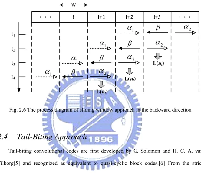
2.3 Sliding Window Approach

As what we described in the previous section, the MAP-based algorithm (including MAP algorithm, Max-Log-MAP algorithm, and Log-MAP algorithm) requires both forward and backward path metric to calculate the log-likelihood ratio. Since the forward and backward recursions start from different initial point, the entire block message has to be received and stored for computing forward and backward recursions. Furthermore, we have to store one of the path metrics of forward or backward recursion and wait for another. These restrictions enlarge the memory requirement for hardware implementation of turbo decoder. For example, the maximum block length of 3GPP standard is 5114, which means 5114 codewords and path metrics should be stored. Besides, long output la

state if the backward recursion goes long enough. Fig. 2.5 and Fig. 2.6 shows the process of this approach in both directions and the detail operating flow is described as follows.

tency is also introduced. It limits the speed and throughput of turbo decoder design.

The main problem is that long block length can not be divided into several shot sub-blocks immediately, since the lack of boundary path metric of sub-blocks in opposite direction of input sequences will degrade the performance. Thus, a sliding window approach was proposed in [27] and later on in [28] to overcome this drawback. This approach utilizes the fact that the backward path metrics can be highly reliable even without knowing the initial

(29)

i i+1 i+2 i+3 L(u )t L(ut) L(ut)

t

1 3 4

t

2

t

W

α

β

1 2

β

1

β

1

β

2

β

1

β

2

β

α

2

β

α

Fig. 2.5 The process diagram of sliding window approach in the forward direction

path metric values for the true backward recursion

First, the received codeword is divided into many sub-blocks, with a sub-block length of

W. W is called the convergence length with typically five times the constraint length of the

encoder. For each sub-block i, the initial path metric values are inherited from the neighbor sub-blocks for both forward and backward recursion operations. Note that in Fig. 2.5 the dummy backward recursion β1 is employed to obtain the initial

β2. Although the initial condition for β1 is unknown except the last

sub-block, we introduce the equal probability condition for β1 values:

1

1 ( )

j

, for all

0,1,...,

t

x

j

M

β

=

_{(2. 31)}

where

x

tj denotes the path metric of j-th state at time t, the last Trellis section of β1 , and M

is equal to the total state number. During the forward recursion α proceeds in the i-th sub-block and stores these values into memory, the dummy backward recursion β1 is

performed in the i+1 sub-block concurrently. As soon as β1 computation is finished, the initial

metrics in the i+1 sub-block are available for β2 metrics in computation, and the

(30)

Fig. 2.6 shows the process diagram of sliding window approach in the backward direction. The operation flow is similar to the forward direction type except for two forward recursions α and one backward recursion β.

β

2

α

1

α

1

α

1

α

2

α

2

α

2

α

1

α

ength code blocks of CCs. The standard solution is to add same bits at the tail of in

Fig. 2.6 The process diagram of sliding window approach in the backward direction

2.4 Tail-Biting Approach

Tail-biting convolutional codes are first developed by G. Solomon and H. C. A. van Tilborg[5] and recognized as equivalent to quasi-cyclic block codes.[6] From the strict definition of convolutional codes (CCs) it is clear that CCs can only be applied to semi-infinite sequences, i.e., encoding starts at time t = 0 in the all-zero state and goes on continuously. But almost any communication system is block-oriented, we must find methods to obtain finite l

formation sequences to force the encoder back to the all-zero state. This method can avoid the weak error protection for the last codeword bits, however it causes same rate loss due to tail bits.

Tail-biting avoids the rate loss without suffering from degraded error protection at the end of the codeword. With tail biting technique, the starting state of encoder is not necessarily

(31)

the all-zero state. It can also be any one of the other states. The fundamental idea behind state after encoding the infor

tail-biting is that the starting state should be the same as the ending

mation sequence, i.e., x₀ =xN. In the Trellis representation of tail-biting codes only

those paths that start and end at the state are valid codewords.

2.4.1 Encoding tail-biting codes using feedback encoders

Let us consider a feedforward encoder first. It is obvious that we only have to consider the last m input k0-tuples of information sequences to fulfill the tail-biting boundary

conditionx₀ =x_N. But the situation is more complicated for feedback encoders. The last

encoding statexN depends on the entire information vector u=( , ,u0 … uN−1). Thus, we must

calculate for a given information vector u the initial statex₀ that will lead to the same state

after N cycle. To solve this problem, we consider the state representation:

1

T

t t

x

₊

=

A

x

+

B

u

_t (2. 32) To solve the iterated function by substitution, we can find that the complete solution of (2.32) equals to the superposition of the zero-input solution and the zero-state solution .

0 t τ − =

A

the in [ ]zi [ ]zs t

x

_t 1 ( 1) [ ] [ ] [ ] 0 0 t t T zi zs t zs t t t t

x

=

x

+

∑

A

− −τ

B

u

_τ

=

x

+

x

=

A

x

+

x

_{(2. 33)}

If we demand that the state as time t=N is equal to itial statex₀, we obtain from

[ ]zs N

(2.33):

N

(

m

)

0

x

=

A

+

I

x

(2. 34) Where I_mdenotes the m-by-m identity matrix. If a feedback encoder with certain information length N can provide an invertible matrix( N )

m

+

A I , the correct initial state x₀ can be

calculated by knowing the zero-state response [ ]zs N x .

(32)

two steps:

First, the encoder starts from the all-zero state with given information sequences to determine the zero-state response . By knowing the zero-state response, we can calculate the corresponding initial state

[ ]zs N x

0

x by (2.34). Second, the encoder starts from the correct initial

statex₀ and a valid codeword results.

Fig. 2.7 The encoder process of tail-biting convolutional code

Since the matrix has to be invertible, not every code length is legal with a given feedback encoder. Moreover, some feedback encoder can not be tail-biting. Some detail discussion can be found in [7], [8], and[9].

( N )

m

+

(33)

Chapter 3 The High Speed Turbo Decoder

Design I

3.1 Introduction

Presented by Berrou et al. in 1993 [1], turbo codes have been recognized as a milestone in the channel coding theory. Due to their outstanding error-correcting capabilities, turbo codes have been highly appreciated in wireless communications, where signal-to-noise ratios (SNRs) are generally low. Two commonly used soft-input–soft-output (SISO) turbo decoding algorithms are maximum a posteriori probability (MAP) algorithm [2] and soft-output Viterbi algorithm (SOVA) [4]. MAP-based turbo decoders are known to have better performance than SOVA-based turbo decoders while having slightly larger complexity.

Many researches are proposed to improve the speed of turbo decoder. Bickerstaff proposed a high radix decoder [11]; Bougard introduced a full-duplex design [12]; Urard implemented a 5 iterations series turbo decoder [16]. Their works increase the throughput by refining the architectures of the SISO decoders. The highly parallel structure might be a solution to substantial improvement, but there are two difficulties that have to be overcome. One is the memory contention problem resulted from high-radix and multiple processing elements; the other is the critical path resided in the add-compare-select (ACS) circuit. We proposed a high speed solution that resolves these two problems by using a novel interleaving methods and modifying the MAP decoders. Some interleaving algorithms with contention-free properties have been published [9], and our design adopts the inter-block permutation (IBP) interleaver [13]. Then we exploit a high-radix MAP decoder with shorter

(34)

critical path to increase data rate [14]. The proposed turbo decoder provides both high throughput capability and outstanding energy efficiency while maintaining equivalent performance as 3GPP turbo code.

3.2 Decoder Structure

For high speed turbo decoder design, there are generally two types of architectures proposed in the state of the art. Fig 3.1 shows these architectures, the series architecture and the parallel architecture. The series architecture duplicates the same number of processing elements as iterations and each processing element decodes the codeword for only one iteration. After decoding, each processing element will pass the extrinsic value to the next element. This architecture is easy to implement but the hardware cost is very high. The parallel architecture decodes one codeword with multiple decoders. This architecture is more flexible since number of decoders varies from different specifications. The major problem of this architecture is that how to decode a block codeword with multiple decoders. The forward recursion and the backward recursion connect the whole codeword, so we should apply some techniques to separate them. In the following, we will introduce our proposed design using the parallel architecture to solve this problem.

(35)

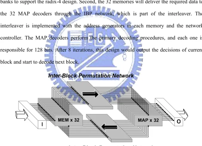
Fig. 3.2 shows the block diagram of proposed decoder, which consists of 32 parallel MAP decoders and 32 parallel memory sets. We separate a codeword into 32 sub-codewords with length 128. Each sub-codeword is assigned to one decoder and decoded separately. These sub-codewords are connected by a well-designed inter-block permutation (IBP) interleaver. This method avoids the forward and backward recursion problem while using the parallel architecture. The decoding process is described as follows: first, each memory will collect a 128-bit sub-codeword from input buffer till the whole 4096-bit codeword is received. The memory stores the received symbols and extrinsic information, which is divided into two banks to support the radix-4 design. Second, the 32 memories will deliver the required data to the 32 MAP decoders through the IBP network, which is part of the interleaver. The interleaver is implemented with the address generators in each memory and the network controller. The MAP decoders perform the primary decoding procedures, and each one is responsible for 128 bits. After 8 iterations, this design would output the decisions of current block and start to decode next block.

Fig. 3.2 Block diagram of proposed turbo decoder

3.3 Interleaver Design for High Speed Turbo Code

3.3.1 Contention-free Interleaver

(36)

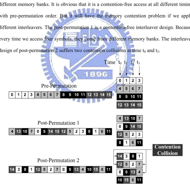
into M size-W windows (N = MW) and employing M synchronous MAP-based decoders with M separate memory banks. Interleaving latency is eliminated by writing the M values generated each clock cycle directly to their interleaved positions. However, if the interleaver is not designed carefully, two or more MAP-based decoders may require access to the same memory bank on a given clock cycle, resulting in a memory contention. Moreover, a high radix decoding structure also suffers from the memory contention problem while accessing multiple codeword symbols from memories. Fig 3.3 shows an example of memory contention problem in a parallel decoding structure. We store a codeword sequence in order in four different memory banks. It is obvious that it is a contention-free access at all different timing with pre-permutation order. But it will have the memory contention problem if we apply different interleavers. The post-permutation 1 is a contention-free interleaver design. Because every time we access four symbols, they come from different memory banks. The interleaver design of post-permutation 2 suffers two contention collisions at time t0 and t3.

(37)

3.3.2 IBP Interleaver

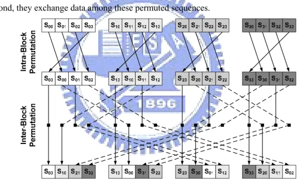
The IBP interleaver in [13] favors both performance and throughput of turbo decoder. Such method guarantees no hazards when multiple MAP decoders try to access multiple memories concurrently. The IBP interleaver consists of two steps of permutation: intra-block permutation and inter-block permutation. The first step rearranges the symbol sequences in each sub-block with the same rule. The second step swaps the sequences between blocks periodically. The destination can be derived by executing bit-wise exclusive-or between the original block index and the IBP parameter. Fig. 3.4 demonstrates an example of IBP interleaver with four sub-blocks. First, all sub-blocks are individually reordered by right rotate; Second, they exchange data among these permuted sequences.

Fig. 3.4 An example of IBP interleaver with four sub-blocks

3.3.3 Butterfly network

The butterfly network is designed to perform the inter-block permutation in the IBP interleaver. This structure also avoids the memory contention problem between sub-blocks and reduces the circuit complexity. Fig. 4 shows the corresponding structure for above example illustrated in Fig. 3. The network is divided into two levels, and each level has one external signal to control the multiplexers. S0 and S1 will define four possible connections. In

(38)

general, the butterfly network links N memories to N MAP decoders by log2N levels of

switches. Each level requires 1-bit control signal to manage its N multiplexers; the total log2N bits establish N possible connections.

Fig. 3.5 A 4x4 butterfly network for IBP interleaver

3.3.4 Double prime interleaver

All the data inside each block will be divided into two groups and be stored in the two separate memory banks. When radix-4 MAP decoders request two symbols at each cycle, these two symbols must be derived from different memory banks. This is another contention problem that should be aware of. Our design uses the double prime interleaver to resolve this problem. The double prime interleaver is constructed by two prime interleavers whose function are expressed by

(( ₂ ) mod ) 2 1, is odd 2 (( ₂ ) mod ) 2, is even 2

( )

{

L i _p _i L i _{p s} _i

i

π

⎢ ⎥×⎣ ⎦ × + ⎢ ⎥× + × ⎣ ⎦

=

(3. 1) This L is the block length, and it must be an even number. Note that p must be relative prime to L/2 and s is a constant shift. Both the interleaver and de-interleaver could be expressed in (3.1) with different parameters. Double prime interleaver with well-searched parameters would outperform the interleaver in 3GPP turbo coding. Most important of all, an well-designed double prime interleaver is an fully contention-free interleaver for certain

(39)

sub-block length. For example, we can choose any factor of the sub-block length as the parallel access number and the memory bank number. It is guaranteed that a well-designed double prime interleaver is a contention-free interleaver.

3.4 High-Throughput MAP Decoders

3.4.1 Retimed radix-2x2 ACS unit

For trellis-based decoders, the branch number of conventional high-radix design increases exponentially however the branch number of the two-stage structure increases linearly. A two-stage ACS is introduced in [14] to ease the area overhead of high-radix ACS. The complexity of ACS unit depends on the branch number, so our design prefers radix- 2 × 2 ACS to radix-4 ACS. But the critical path of two-stage structure is longer than conventional structure. The recursive property of path metric would make the pipelining method inefficient here, however, the critical path can be reduced by our proposed retiming method.

It is obvious that the ACS unit could not execute compare-select operations until addition results are ready; such data dependency restricts the operating frequency. To eliminate the dependency, the data path of ACS unit must be modified. So the proposed decoder applies the retiming technique, and Fig. 3.6 demonstrates the procedure of a retimed radix-2× 2 ACS. The first step shown in Fig. 3.6(a) is retiming of registers. Move and duplicate the registers ahead of the compare circuits, then computation order is rearranged from add-compare-select to compare-select-add. The registers have to store the summation of path metric and branch metric rather than only path metric. The second step shown in Fig. 3.6(b) is relocation of adders. Move and duplicate the adders ahead of the multiplexers; now the compare-select and addition could execute concurrently. The modified ACS unit is shown in Fig. 3.7, where the critical path becomes two consecutive compare-select operations. It would cause extra area overhead because of double registers and double adders, and the improvement of the radix-2×2 architecture could compensate for this loss. The relocated method can accomplish

(40)

not only high-speed but area-efficient solution.

Fig. 3.6 Retiming procedure of a radix 2x2 ACS unit

(41)

3.4.2 The circuit for log-likelihood ratio calculation

Our design adopts the modulo normalization to avoid overflow of path metric [15]. This method requires only one more bit in the ACS unit and a simple modification inside the LLR unit; there are no specific circuits for normalization in ACS unit. Only the differences between forward path metrics and the differences between backward state metrics are significant in modulo normalization, so the LLR unit has to use these differences to calculate the log-likelihood value. Our design rearranges the computation order of log-likelihood value from circuit in Fig. 3.8(a) to circuit in Fig. 3.8(b). Although the two circuits have the same function, but original circuit may result in overflow due to the limited data width. The modified circuit could guarantee the correctness and cause no extra path delay.

Fig. 3.8 The circuit for log-likelihood calculation

3.5 Simulation Result and Chip Implementation

The proposed turbo code with code rate 1/2 could decode 4096 bits after 8 iterations, and the implementation applies maximum log-MAP algorithm with a scaling factor 0.75. The other specifications are listed in Table. 3.1. Fig. 3.10 and Fig. 3.11 shows the performance comparison between the proposed code and 3GPP turbo code. The floating point and the fixed point simulation result are both competitive to the result of 3GPP standard. However, the proposed turbo design has better distance property due to the interleaver design than the 3GPP

(42)

standard. Obviously, the 3GPP standard suffers from the error floor phenomenon more than the proposed design.

(43)

(44)

Table 3.1 Turbo Decoder Specification

Algorithm Max-Log MAP

ACS unit Radix 2x2 (retimed)

Code polynomial 3 2 3 1 1 1 D D D D ⎡ + + ⎤ ⎢ ₊ ₊ ⎥ ⎣ ⎦

Interleaver IBP interleaver (p, s) = (15, 23)

Sliding Window 32

Code Rate 1/2 (punctured)

Block length 4096(128 x 32) Quantization 6 bits (3.3) iteration 8 Scaling Factor 0.75 Note Tail-Biting Technology 0.13um 1P8M

Clock rate 250MHz /w DLL 80MHz/wo DLL *

Throughput 500Mbps 160Mbps *

Gate count 2.67M

Core Area 17.8 mm2

power 762mW 275mW *

nJ

/

bit‧iteration 0.19 0.22 *

The decoder chip is fabricated with a 0.13µm 1P8M CMOS technology, and the die photo is shown in Fig. 3.12. The core area is 17.8mm2 with 2.67M gates count, including the 3.33mm2 memory block. A delay lock loop (DLL) circuit is applied to generate internal clock

(45)

source as four times the external frequency. The design could operate at 250MHz with the help of DLL during post-layout simulation, due to the relocation technique. However, the DLL could not work as expected during measurement. The test chip could achieve 160Mb/s and 275mW power consumption with 1.32V supply. For the decoder with 8 iterations, the energy efficiency is 0.22nJ/b/iter. Table II lists the comparison of the proposed code with other published works, and the proposed design has the optimal energy efficiency [11][12][16].

Output Buffer

DLL

(46)

Table 3.2 Comparison with Other Turbo Decoder proposed [11] [12] [16] Technology 0.13μm 0.18μm 0.18μm 0.13μm Clock rate 80MHz 145 MHz 160 MHz 352 MHz Throughput 160Mbps 24 Mbps 71.7 Mbps 352 Mbps Block Size 4096 5114 384 2048 Core Area 17.8mm2 14.5 mm2 7.16 mm2 10 mm2 power 275mW 1450mW N/A 2464mW Energy Efficiency 0.22 nJ/bit‧iter 10.0 nJ/bit‧iter 9.7 nJ/bit‧iter 1.4 nJ/bit‧iter

3.6 Summary

The proposed turbo decoder with the parallel architecture enables multiple processing elements to decode one codeword concurrently. The proposed IBP interleaver connects all processing elements in the parallel architecture and avoids the limit of the forward and backward recursions. We also introduce a high speed methodology for high radix decoder structure. The combination of two stages ACS and the retiming technique efficiently speed up the decoding throughput with acceptable hardware cost. The energy efficiency of proposed turbo decoder is much smaller than that of the state of the art.

(47)

Chapter 4 The High Speed Turbo Decoder

Design II

In chapter 3, we have introduced a power efficient turbo decoder design with 32 processing elements. The throughput of the proposed design is about 500Mbps in pre-layout simulation. The critical path of the proposed design is the ACS units. However, the throughput of a radix 2x2 ACS unit working under 250MHz is 500Mbps and the total throughput of the decoder should be 1Gbps with 32 processing elements under 8 iterations. The total throughput is reduced by the following two issues:

z One block is calculated twice due to the tail-biting. The calculation of α recursion of first

block introduces a dummy sub-block and reduces the throughput.

z Due to the iterative decoding and the interleaver of turbo code, the decoder must stop

and wait until the processed data stored in the memories. This data hazards happen twice per iteration between two different decoding rounds.

These issues will be discussed in detail in the following sections. We will propose methods to solve these problems and implement a 1Gbps high throughput and power efficient turbo decoder.

4.1 Introduction

4.1.1 Data Hazards

There is an iteration bound occurred in the MAP-based decoder structure, so the forward and backward recursion in a turbo decoder is always the critical path and occupy a large area in the implementation. This is a main reason that the hardware of the forward and backward

(48)

recursion is always reused. The cycle-based decoding procedure is shown in Fig. 4.1. This example shows a sub-block size 16 and a radix 4x4 decoder decodes 4 symbols each cycle. It shows that the forward and backward recursion modules and the LLR module are reused for four cycles. Furthermore, the pipelined method can be used while decoding different sub-blocks because there is no data dependency between different sub-blocks in the same decoding round. Fig. 4.2 shows the case we proposed in chapter 3 and a data hazard happens while decoding. The data dependency results from the interleaver between sub-block 4 in the pre-decoding round and sub-block 1 in the post-decoding round. The extrinsic information of sub-block 4 in pre-decoding round may be used in sub-block 1 in post-decoding round. This is the reason why the decoder should be idle until the extrinsic information stored in the memories.

Fig. 4.1 A cycle-based decoding procedure

Fig. 4.2 A data hazard occurred while decoding

4.1.2 A dummy sub-block

A valid codeword in the tail-biting Trellis makes the encoder to start and end at the same state, instead of zero state only. Therefore, a dummy sub-block, as well as the last sub-block, will be calculated first to estimate the initial value of the forward recursion of the first sub-block. Decoding schedule of a sub-codeword is shown in Fig. 4.3 and Fig. 4.4. We can

(49)

easily find that the data hazard and the dummy block make the decoding procedure longer. It takes 128 cycles to decode a sub-codeword and the utilization of the hardware is 50% only. The decoder is idle for 12 cycles and some modules are idle while other modules are calculating. Therefore, the working duration of the forward and the backward recursion modules and the LLR module is 64 cycles.

Fig. 4.3 Decoding schedule of a sub-codeword

Interleaved

Sub-block

Idle 16 cycles

Total 128 cycles

… …

Fig. 4.4 Decoding schedule of previous design

4.2 Decoding Schedule

The data hazard and the dummy sub-block cause a 50% degradation of the throughput. In this section, we will propose a method to solve this problem and make the 100% utilization of the hardware.

4.2.1 Decoding with two codewords

Due to the data dependency of pre-decoding round and post-decoding round connected by the interleaver, a better way to break this relation is to decode two codewords alternately.

(50)

The proposed method achieves 100% hardware utilization without any extra logic cost. The only cost of this method is that we have to store two codewords in the memories. The detail procedure in Fig.4.5 is described as follows:

z Decode from the first sub-block and get the initial value of forward recursion of the

first sub-block from the previous iteration. If it is the first iteration, then set an all zero initial value for beginning.

z Store the initial value needed by the next iteration, so it is not necessary to calculate

the dummy sub-block.

z First, decode the pre-permutation sequences of sub-codeword A. z Second, decode the pre-permutation sequences of sub-codeword B. z Third, decode the post-permutation sequences of sub-codeword A. z Decode the post-permutation sequences of sub-codeword B. z Then decode alternately until the last iteration.

Fig. 4.5 Decoding schedule with two codewords There are two more steps should be noticed about the dummy block:

z While decoding each sub-codeword, decode from the first sub-block and get the

initial value of forward recursion of the first sub-block from the previous iteration. If it is the first iteration, then set an all zero initial value for beginning.

(51)

z Store the initial value needed by the next iteration, so it is not necessary to calculate

the dummy sub-block. The dot line in Fig. 4.5 shows where we store the initial value and where we read the initial.

The fundamental idea of our proposed method is to keep the hardware calculating and avoid to calculate the same sub-block twice. Notice that at any timing frame all hardware modules are working, which means the hardware utilization reaches 100%. Applying the method, we can double the throughput by reducing the decoding cycles from 128 to 64 for each sub-codeword, but the extra storage of initial values is about 6144 bits in the case of our proposed design in chapter 3.

4.3 MAP Decoders

4.3.1 The structure of each processing element.

It is mentioned in section 3.4 that the number of the processing elements and the throughput of each element are two main factors of the total throughput. In addition to adding the number of processing elements, the throughput of each element should increase for a high throughput turbo decoder design. The method we used in the new proposed design is a higher radix Trellis structure.

For any Trellis-based decoder, two important factors should be considered carefully are the number of states and the branch number of each state, which affect the implementation complexity numerously. While applying a high radix design, another dimension should also be taken into account is the stage number of Trellis. In Fig. 4.6, both radix 16 and radix 4x4 Trellis diagram merge 4 stage Trellis diagram into one. The radix 16 Trellis has 16 branches for each state. The radix 4x4 Trellis has 4 branches for each state, but it is a two stage structure. However, the total branch number of the radix 4x4 is half of the radix 16. Therefore, the hardware of radix 16 is twice as that of radix 4x4.

(52)

16

Radix 16 Radix 4x4

Fig. 4.6 Radix 16 and radix 4x4 Trellis diagram

Fig. 4.7 shows the hardware cost of two structures. We can find that the number of comparators and multiplexers of the radix 4x4 structure is twice as that of the radix 16 structure, but the complexity of a 4 to 1 comparator is much smaller than that of a 16 to 1 comparator. Besides, the branch number of the radix 4x4 is less than that of the radix 16. The new proposed design uses the radix 4x4 structure in each processing element.

(53)

4.3.2 The memory units

Considering the radix 4x4 structure and the storage of two codewords, the memory units of the turbo decoder should be redesigned. First, the memory should be divided into four banks and each bank consists of five sub-banks. The division of the memory units is due to the bandwidth and contention. We have to access four input symbols for the processing element at each cycle and each symbol consists of information bits, parity bits and the extrinsic part. Fig. 4.8 shows one memory unit in detail. Notice that each bank in the memory unit is the same as that mentioned in chapter 3, but the number of banks is double and the bandwidth is also double. Furthermore, the total storage is double because of the additional codeword B.

Fig. 4.8 The memory unit

4.3.3 Retime or not retime

In chapter 3, we have introduced a retiming technique to shorten the critical path for a two stage ACS structure. The retimed structure has more hardware costs than the no retiming version. The critical path comparison between these two versions is shown in Fig. 4.9, and the target technology of our implementation is the UMC 90 nanometers process. Obviously, the

Gbps高速渦輪碼之設計與實現

國立交通大學

電子工程學系 電子研究所碩士班

碩 士 論 文

Gbps 高速渦輪碼之設計與實現

Design and Implementation of Gbps Turbo Decoders

學生 ： 賴名威

指導教授 ： 李鎮宜 教授

Gbps 高速渦輪碼之設計與實現

Design and Implementation of Gbps Turbo Decoders

研 究 生：賴名威 Student：Ming-Wei Lai

指導教授：李鎮宜 Advisor：Chen-Yi Lee

國 立 交 通 大 學

電子工程學系 電子研究所 碩士班

碩 士 論 文

Gbps 高速渦輪碼之設計與實現

學生：賴名威 指導教授：李鎮宜 教授

國立交通大學

電子工程學系 電子研究所碩士班

摘要

Design and Implementation for Gbps Turbo Decoders

Student : Ming-Wei Lai Advisor : Dr. Chen-Yi Lee

Institute of Electronics Engineering

National Chiao Tung University

ABSTRACT

誌 謝

Contents

List of Figures

List of Tables

Chapter 1

Introduction

1.1 Motivation

1.2 Thesis Organization

Chapter 2

Turbo Code

2.1 Principle of Turbo code

2.1.1 Turbo Encoding

2.1.2 Turbo Interleaver

2.1.3 Turbo Decoding

2.1.4 Error floor effect

2.2 Decoding Algorithms for Turbo Code

2.2.1 The MAP algorithm

∑

∑

∑

∑

∏

∏

∑

∑

∑

∑

∑

∑

∑

2.2.

2 The Log-MAP algorithm

(

)

(

)

(

)

(

)

2.2.3 The Max-Log-MAP algorithm

(

)

(

)

∑

∑

(

)

(

)

(

)

(

)

電子工程學系電子研究所碩士班

碩士論文

學生：賴名威

指導教授：李鎮宜教授

研究生：賴名威 Student：Ming-Wei Lai

國立交通大學

電子工程學系電子研究所碩士班

碩士論文

學生：賴名威指導教授：李鎮宜教授

電子工程學系電子研究所碩士班

誌謝