新穎影像重建演算法暨其系統晶片設計應用於連續波式擴散光學斷層掃描系統

國

立

交

通

大

學

電子工程學系

碩

碩

碩

碩

士

士

士

士

論

論

論

論

文

文

文

文

新穎影像重建演算法暨其系統晶片設計應用於

連續波式擴散光學斷層掃描系統

Novel Image Reconstruction Algorithm and System-on-Chip Design for

Continuous-wave Diffuse Optical Tomography Systems

研 究 生： 徐源煌

指導教授： 方偉騏 教授

桑梓賢 教授

中

中

中

中

華

華

華

華

民

民

民

民

國

國

國

國

九

九

九

九

十

十

十

十

八

八

八

八

年

年

年

年

六

六

六

六

月

月

月

月

新穎影像重建演算法暨其系統晶片設計應用於

連續波式擴散光學斷層掃描系統

Novel Image Reconstruction Algorithm and System-on-Chip Design for

Continuous-wave Diffuse Optical Tomography Systems

研究生:

徐源煌 Student：Yuan-Huang Hsu

指導教授:

方偉騏 Advisor：Wai-Chi Fang

桑梓賢 Advisor：Tzu-Hsien Sang

國 立 交 通 大 學

電 子 工 程 學 系

碩 士 論 文

A Thesis

Submitted to Department of Electronics Engineering & Institute of Electronics College of Electrical and Computer Engineering

National Chiao Tung University In partial Fulfillment of the Requirements

for the Degree of Master of Science

in

Electronics Engineering June 2009

致

致

致

致

謝

謝

謝

謝

我是個幸運的人，在研究的路上一直有兩位優秀的指導老師給予指導與協助， 感謝 方偉騏老師與 桑梓賢老師兩年來的教誨與包容，從方偉騏老師身上，我在 課業上、研究上、與待人處事上均獲益良多，研究過程中老師總是鼎力協助。儘 管非常忙碌也一定會撥空或是利用餐敘的時間與我討論研究方向與進度，有時您 因為國際會議在國外，也會利用視訊與學生開會並給予指導，非常感謝您的辛勞。 桑老師常常耐心的與我討論研究內容與陪我一起思考問題的解決方式，每次精準 的問題也讓我可以發現更多研究的空間與盲點，感謝老師。我還有很多方面要與 兩位老師學習，因為自己還有許多不足之處，在未來一定也還要抓住與兩位老師 學習的機會。 同時也要感謝我的口試委員 趙昌博教授與 范倫達教授給予我論文內容的 指導與討論，讓本論文與研究因為有兩位教授的參與更加完美。也感謝兩位老師 的不辭辛勞的參與口試與論文指導，使學生備感榮幸，收獲滿滿。

接著我要感謝實驗室學長(秋國學長、盛弘學長、翔琮學長與凱信學長)，感 謝你們參與討論、工作站上協助與經驗的傳承。尤其感謝翔琮學長，給予硬體設 計上的指導與協助，我們常常在深夜的實驗室，同時都在為自己的研究努力。感 謝實驗室同學與學弟(詔凱、志文、致中、宗翰、少彥與鴻溝)，與你們一起為計 劃努力與互相學習是件很開心的事情，也特別感謝致中在系統雛型建置上一起做 的努力與貢獻。感謝同處在同一間辦公室的學長與同學在研究上的討論與協助 (建螢、燦文、偉豪、曉涵與書餘)。 此外，也要感謝北翰科技的薛岱方先生與美商國家儀器的林逸帆先生、黃翔 鉎先生在儀器使用上的指導與教學。 最後，我要感謝我的父母親與我的妹妹。在求學的路上一路支持與鼓勵，沒 有你們我也就沒有現在的我，謝謝爸媽的辛勞與養育，也謝謝妹妹與小遙在我苦 悶時的關心與鼓勵。我幸運是因為有老師與大家的提攜，謝謝你們。

摘

摘

摘

摘

要

要

要

要

本論文針對連續波式擴散光學斷層掃描術之影像重建演算法，提出擁有較低 運算複雜度的區塊重建模式，並對此新穎的重建演算法進行模擬與精確度分析， 最後將之實現於超大型積體電路。 擴散光學斷層掃瞄為一非侵入式醫學造影術，使用光源為 650nm-950nm 之 近紅外光波段的擴散光源，利用不同生物組織對近紅外光光譜不同的分佈與相關 資訊，偵測生物體內組織之光學特性與成分濃度在空間與時間的變化或是絕對量， 如:吸收係數、擴散係數、含氧血紅素濃度、非含氧血紅素濃度以及血氧飽和度 等…。 近年來，擴散光學斷層掃描系統在臨床應用上有，大腦功能性造影、胸部腫 瘤檢測以及其他醫學相關領域。此技術有非侵入、及時檢測、非輻射源等優點， 其中連續波式系統擁有良好的可攜性、造價低廉與快速檢測等優點，如可將影像 重建演算法複雜度降低並實現於系統晶片之中，並配合手持式裝置與無線模組， 可將此醫學影像技術更廣泛的使用。 本研究目的分為兩大部分，第一部分著重於不同影像重建模式的模擬與分析， 以求在降低運算量與使用有限的資訊來源限制下重建出精確的影像，模擬的模型 為兩不同吸收係數的非均勻吸收體位於均勻的吸收體中，在幾何形狀與位置不同 的條件情況進行影像重建，並利用 Mean Square Error 分析影像的精確度。第 二部分，選擇 Jacobi 奇異值分解演算法執行影像重建過程中的反向解並將 Jacobi 奇異值分解演算法實現於電路，應用 MATLAB 做硬體資源需求的評估與考量， 最後使用 FPGA 做為功能的驗證。 未來，此醫學影像重建引擎可配合其他醫學訊號處理引擎，像是腦波訊號與 心電訊號共同實現於系統晶片。使系統縮小化成為醫療用途的可攜式裝置，並應 用於緊急救護、醫療檢測儀器、臨床檢測與遠端照護，為人類帶來更多福祉。 關鍵字 關鍵字 關鍵字 關鍵字:::: 近紅外光斷層掃描術、奇異值分解、近紅外光光譜、醫學影像

Abstract

This paper proposes a low computational overhead image reconstruction algorithm of continuous wave diffuse optical tomography (CW-DOT) which is called sub-frame reconstructed mode. The novel reconstruction algorithm was simulated and its accuracy analyzed. Moreover, it was implemented on very large scale integrated circuit.

DOT is a non-invasive medical imaging technique and uses near infrared optical source with wavelength within 650nm-950nm. By the different distribution of near infrared spectroscope (NIRS) within distinct biological tissue, the spatial and temporal change and absolute values of biological characteristics can be obtained such as absorption coefficient, scattering coefficient, concentration of oxy-hemoglobin and concentration of de- oxy-hemoglobin.

Recently, the clinical applications of DOT are in functional image reconstruction of the brain, detection of tumor in breast, and others. Non-invasive, real-time and not a source of radiation are the beneficial features of DOT. Furthermore the CW-DOT systems have small volume, low cost, high speed and other advantages. If the image reconstruction algorithm can be decreased the complex and implemented on SoC, then through cooperation with handheld instrument with wireless module, the DOT system can be more convenient to put in use in real life applications.

There are two focuses in this research. The first one aims to reduce the complexity of algorithm and reconstruct accurate image with the finite information by simulating and analyzing the different reconstructed way. Distinct geometry and location of inhomogeneous absorbers were allocated in homogenous absorbers to do simulation. Mean Square Error (MSE) was used to compare the accuracy of images. The second issue is choosing the algorithm to implement. After survey, the Jacobi

Singular value decomposition was chosen to realize the inverse solution of reconstruct process and realize on hardware description language (HDL). MATLBA is used to evaluate the hardware resources. Finally, FPGA will be used to do the function identification of the image reconstruction processor.

In the future, the image reconstruction processor can be accompanied with other biomedical signal processors such as electroencephalography (EEG) or electrocardiograph (ECG) and be implemented on SoC. The urgent image modality, clinical diagnosis and bed-side monitor, real-time inspection and remote care can be made by minimizing these medical systems to handheld apparatus and bring the more welfare to our human life.

Keywords: diffuse optical tomography, singular value decomposition, near infrared

Contents 致謝 ……… i 摘要 ……… ii Abstract ……… iii Contents ……… v List of figures ……… vi

List of tables ……… vii

Chapter 1 Introduction ………. 1

1.1. Medical imaging………. 1

1.1.1 Invasive medical imaging ……….. 1

1.1.2 Non-invasive medical imaging………... 1

1.2. Singular value decomposition algorithm………... 6

1.3. Overview of the proposed prototype of CW-DOT system…… 7

1.4. Scope and contributions of this research……… 9

Chapter 2 Diffuse Optical Medical Imaging Technique………. 12

2.1. Photon migration ………... 12

2.2. Near-infrared ray spectroscope……….. 14

2.2.1 Modified Beer-Lambert Law………... 14

2.2.2 Application and implementation of NIRS…………... 16

2.3. Diffuse optical tomography………... 17

2.3.1 Diffusion equation………. 18

2.3.2 Application and implementation of DOT………... 19

2.4. Review of this study and recent works………... 22

Chapter 3 Image Reconstruction Algorithm and Processor………….. 26

3.1. Forward model………... 26

3.2. Inverse solutions………. 28

3.2.1 Jacobi SVD algorithm……….... 29

3.2.2 Truncated SVD………... 31

3.2.3 Frame mode and sub-frame mode………... 32

3.3. The result of software simulation and analysis……….. 32

3.4. The design of image reconstructed processor………... 37

3.4.1 The architecture of processor………. 37

3.4.2 Memory controller………. 39

3.4.3 The spec of the JSVD processor……….... 41

Conclusion ……… 42

List of figures

Figure 1.1 A typical MRI facility………... 3

Figure 1.2 A schema of a PET acquisition process……… 3

Figure 1.3 Standard OCT scheme is based on a low time-coherence Michelson interferometer………. 4

Figure 1.4 A scheme of the homemade prototype………. 8

Figure 1.5 Figure 1.5 Overview of the proposed CW-DOT system. (a) User Interface of CW-DOT system. (b) A set of sensor networks. (c) Power supply and DAQ card of NI PXI system. (d) FPGA platform. (E) The flow of emulation……… 10

Figure 2.1 Different types of travel paths of photon migration………. 13

Figure 2.2 Spectrum of absorption coefficients of HbR, HbO2 and H2O….. 13

Figure 2.3 One channel NIRS system……… 15

Figure 2.4 The modality of TD-DOT systems………... 19

Figure 2.5 The modality of FD-DOT systems………... 20

Figure 2.6 The modality of CW-DOT systems……….. 21

Figure 2.7 (a) Schematic drawing of a high-speed laser Doppler blood flow imager. (b) Blood flow-related images of human fingers. Images size is 512x512………. 22

Figure 2.8 (a) Pulse Oximetry (b) CW-DOT system of NIRx company…... 23

Figure 2.9 (a) Sensor attached on the hat. (b) LED and photo-diode……… 24

Figure 2.10 (a) Hitachi ETG-7100 (b) Array of sensor network………. 24

Figure 2.11 Concept of DYNOT. The input arrows indicate the direction of light……….. 25

Figure 3.1 The relation between sub-frames and one frame………. 32

Figure 3.2 The flow chart of simulation……… 33

Figure 3.3 The distribution of sources and detectors………. 33

Figure 3.4 Two inhomogeneous medium with different location. (a) Th first medium. (b) The second medium……….. 34

Figure 3.5 (a) Frame mode with t=18. (b) Frame mode with t=24………… 34

Figure 3.6 (a) Sub-Frame mode with t=3. (b) Sub-Frame mode with t=4…. 34 Figure 3.7 (a) Frame mode with t=6. (b) Frame mode with t=12………….. 35

Figure 3.8 (a) Sub-Frame mode with t=1 (b) Sub-Frame mode with t=2….. 35

Figure 3.9 The simplified, general bock diagram of architecture………….. 37

Figure 3.10 The basic architecture of CORDIC engine………... 38

Figure 3.11 The example of different data types………. 40

Figure 3.12 The first renew flow of the data input……….. 40

List of tables

Table 1 Different categories of tomography……….. 6

Table 2 The specifications of the home-made prototype……….. 9

Table 3 Pros and cons of different types of DOT systems……… 21

Table 4 Relative researches about NIRS and DOT………... 23

Table 5 The two modes of CORDIC………. 31

Table 6 Compute time and MSE of frame mode……….. 36

Table 7 Compute time and MSE of sub-frame mode……… 37

Chapter 1 Introduction

1.1 Medical imaging

Medical imaging has become one of the most important techniques to help doctors perform accurate diagnosis and obtain more information from patients. By the ways of imaging, it can be divided into two categories: invasive medical imaging and non-invasive medical imaging. This section introduces some commonly used medical imaging in hospitals.

1.1.1 Invasive medical imaging

Invasive medical imaging means a way to destroy the recent state to obtain the biological tissue. For example, biopsy is a way to cut a section by doing a surgical operation or stab a needle into tissue. The section will be examined by a professional pathologist. Biopsy is usually used to inspect tumors of tissue such as skin, breast, or other organs. Sometimes biopsy is also executed to check surgical results.

Another technique is named endoscope but the level of invasion is lower. The endoscope is a method to put a thin fiber into a patient’s body and the images are transferred by the fiber. Doctors have to perform the surgery to open a small hole to set the fiber occasionally. Recently, the core of the fiber was made an empty channel to let a robotic arm go into the body to do operate on patients.

Invasive medical imaging makes the patients suffer from unnecessary pain and harm the patients’ body. Although in special circumstances invasive medical imaging has to be used, in most situations non-invasive imaging can be a better choice.

1.1.2 Non-invasive medical imaging

The oldest non-invasive medical imaging technique was invented after Roentgen devised the X-rays. X-rays have ability to pass through human body directly as same as transparent glass but it contain harmful radiation. Diagnosing pathological changes

of bone and soft tissue are the most important applications of X-rays.

As technology and medical science progress, computed tomography (CT) has replaced the X-rays. CT generates three-dimensional images of an object from a large series of two-dimensional X-ray images taken around a single axis of rotation  by  digital image processing [1]. Its advantages are high speed, high spatial resolution and can be used to exam most parts of body. However, the great bulk and the expensive cost are the main drawbacks of CT.

Another developed imaging technique is magnetic resonance imaging (MRI). MRI provides much greater contrast of image between the distinct soft tissues with no ionizing radiation. The imaging theory of MRI is introduced as follows. Biological tissues are mainly composed of water molecules which each contain two hydrogen nuclei or protons[2]. When a person goes inside the powerful magnetic field of the scanner these protons align with the direction of the field. Radio frequency (RF) fields are used to systematically alter the alignment of this magnetization, causing the hydrogen nuclei to produce a rotating magnetic field detectable by the scanner. This signal can be manipulated by additional magnetic fields to build up enough information to construct an image of the body.

The diseased tissue, such as tumors, can be detected because the protons in different tissues return to their equilibrium state at different rates. By changing the parameters on the scanner this effect is used to create contrast between different types of body tissue. MRI is particularly useful to imaging in neurological conditions because the variation of de-oxy-hemoglobin and oxy-hemoglobin can be detected. When a neuron is activated the de-oxy-hemoglobin around it will increase comparatively to rest state. MRI is also applied on scanning disorders of the muscles and joints, for evaluating tumors and showing abnormalities in the heart and blood

vesse MRI MRI scann introd T indire radio circul biolo the tr positr annih movi they simul do no els. A patien to scan bec is long scan ner is show duced. The positron ectly by a po active tracer lation to co gically activ racer becom ron emissio hilates with ng in oppos create a b ltaneous det ot arrive in p Figure 1.1 A nt who has b ause of the n time and wed in Figur n emission t ositron-emit r isotope is i onduct the s ve molecule me concentr on decay an an electron site direction burst of lig tection of the pairs. A schem A typical MR been implan strong magn inability to re 1.1. Next tomography tting radionu injected into scan [3]. Th .  After it is rated in tiss nd emits a n, producin ns. When the ght and can e pair of pho ma of a PET RI facility. nted with me netic field o construct re t, nuclear m y (PET) dete uclide (trace the living su he tracer is administere sues of inte positron. T ng a pair of ey reach a sc n be detect otons and th T acquisition Figure 1. etal instrum f MRI. The eal-time ima medicine sca ects pairs of r). Before sc ubject which s chemically d and waits rest, the ra The positron f annihilatio cintillator in ted. The te he scanner ig n process is p 2 A schema proc ments isn’t ab main shortc aging. A clin an techniqu f gamma ray canning, a s h is usually i y incorporat typically an dioisotope u n will encou on (gamma) n the scannin chnique de gnores photo presented in of a PET ac cess. Scintill ble to use coming of nical MRI ue will be ys emitted short-lived into blood ted into a n hour for undergoes unter and ) photons ng device, pends on ons which Fig. 1-2.   quisition l

The medical imagings presented above were developed throughout several decades and have been applied on clinical applications widely. Following are newer techniques: optical coherence tomography (OCT) and diffuse optical tomography (DOT) will be briefly presented. In OCT systems, low-coherence light source is used. The beam of light is split by a beam splitter and a beam of light travels along the reference axis while the other one goes toward the tissue [4]. These two light will meet again on mirrors by the beam splitter. If the difference of their travel distances is smaller than the coherence length, it causes the interference. The 3-D images can be obtained by cooperation with the depth scan of reference mirror and lateral scan of objective mirror. The standard scheme of OCT is shown in Fig. 1-3. Though the resolution of OCT is superior to other medical imaging which is about several micrometers and millimeters depth of tissue, the shallow depth is the main shortcoming of OCT. The technique is applied in skin and eye medical area mainly.

The last one to be introduced is diffuse optical tomography (DOT), at the same  

Figure 1.3 Standard OCT scheme is based on a low time-coherence Michelson interferometer [4]. LS=low time-coherence light source; PC=personal computer

time DOT is the main focus of this thesis. The optical source of DOT is within near-infrared wavelength. Because the relative weak absorption by biological tissue, the photons of near-infrared ray can transport deep into several centimeters of tissue [5]. Different elements of human tissue have dissimilar ability to absorb photons, thus DOT reconstruct the characteristics of tissues by detecting the diffuse photons. DOT systems can provide the change of concentration of oxy-hemoglobin (Hb), de-oxy-hemoglobin (HbO2) and optical parameters such as absorption coefficient and

scattering coefficient which are other imaging methods can’t obtain[6, 7].

By using multi-channels of optical sources and detectors, the result of optical parameters can be mapped on the region of object. The application of DOT is extensive from functional brain imaging to tumor detection. The forward model and inverse solution are two critical processes to reconstruct image. The forward model describes how the photons migrate in highly scattering medium and the inverse solution resolves optical characteristics of the medium. There is more detail description of these procedures.

After all, the non-invasive medical imaging techniques can be classified in three sorts by the way of imaging processing. The first way is recording the decay of the straight light from the optical sources to the detectors and reconstruct by the back-project algorithms. The second way employs array of optical sources and detectors which are allocated around the object to detect photons. The travel paths of photons are unknown and the diffusion model is usually used to describe the path of light. The reconstruction images can be obtained by the model and diffuse photons. The last one is very different to the former techniques. The light beams are not needed to pass across the objective such as OCT. Table1 shows these techniques of non-invasive tomography.

1.2 Singular value decomposition (SVD) algorithm

The inverse solution is a procedure of image reconstruction of DOT. Although the multi-channels of sensors can acquire more optical information, the inverse solution still suffers from ill-posed and underdetermined condition. There are some algorithms to deal with the inverse problems such as simultaneous iterative reconstruction technique (SIRT) [8], algebraic reconstruct technique (ART) [9], singular value decomposition (SVD) [10], conjugate gradient algorithm (CG) [10] and others. SVD has been proved that it is superior to other method in localization of in homogeneities and estimation of their amplitude.

In linear algebra, SVD is an important algorithm to deal with matrix factorizations of real or complex rectangular matrix. Its application is wide from digital image processing to principal component analysis (PCA), latent semantic analysis (LSA) …etc [11]. SVD provides very robust quantitative information of a

Table 1 Different categories of tomography [1].

Back-project Method Possibility Method Directly Measure Method

Computed tomography (CT) Positron emission tomography (PET) Single-photon emission computed tomography (SPECT) Electron tomography(ET) Ultrasound tomography (UT) Optical projection tomography (OPT) Electrical resistance tomography(ERT) Electrical capacitance tomography (ECT) Electrical impedance tomography(EIT) Magnetic induction tomography (MIT) Diffuse optical tomography (DOT) Fluorescent molecular tomography (FMT) Optical coherence tomography (OCT) Confocal tomography(CM) Ultrasound biomicroscopy (UBM) Other Method Magnetic resonance imaging (MRI)

matrix and it has proven to have outstanding performance to deal with pseudo inverse, least squares fitting of data, matrix approximation and also problems of ill-posed condition.

A matrix A∈ m n× could be factorized to Eq. (1) by the definition of SVD.

T m n m m m n n n

A_× =U _× D _×V_× (1)

The m m

U∈ × and n n

V∈ × are orthogonal matrix which are T

U U =I and

T

V V = . The columns of I U_{m m}× and

V

n n× are the eigenvectors of T

AA and A AT . The D∈ m n× is a diagonal matrix with nonnegative diagonal elements

σ

_i. The numbers of the singular values are m and it can be represented as

(

1, 2,

)

i m

σ

=

σ

σ

σ

arranged by decreasing order.

There are many numerically stable algorithms for computing the SVD: for instance, Jacobi algorithm, the QR method and the one side Hestenes method. Among these methods Jacobi SVD has features of simplicity, regularity, and local communication for parallel computation. It is also superior to other method to implement on very large scale integrated circuits (VLSI).

1.3 Overview of the proposed prototype of continuous wave diffuse optical tomography (CW-DOT) system

The continuous wave DOT (CW-DOT) system is one approach way to implement DOT. It can be made portable, low-cost, and low-power. For these reasons, this study proposed a homemade prototype CW-DOT system to emulate the novel image reconstruction algorithm.

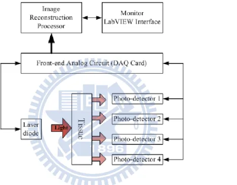
The system is divided into four parts which are sensor networks, front-end circuits, back-end signal processor, and monitor. Fig 1.4 presents the scheme of the system. The sensor network provides the array of the optical sources and the detectors.

The functionalities of front-end circuit’s are convert the analog signals to digital signals, control the sensor networks and reduce the noise with filters built in. The image reconstruction processor is designed to operate the computation of inverse solution. Finally, the result of images can be shown on a monitor of personal computer or handheld devises. The first version is only includes one set of sensor networks which has one laser diode and four detectors.

This prototype is composed of one optical source with 650nm wavelength and uses light-to-voltage converter detectors mounted on an ultra-thin flexible board. The NI PXI-6251 data acquisition card is used to replace the front end circuits to acquire the analog signals from the detectors. The image reconstruction processor is implemented on the Field Programmable Gate Array (FPGA) which model is VIRTEX-4 XC4VLX60 manufactured by XILINX. The result will be shown on the personal computer by LabVIEW 8.5. Table 2 is the specification of the homemade CW-DOT system.

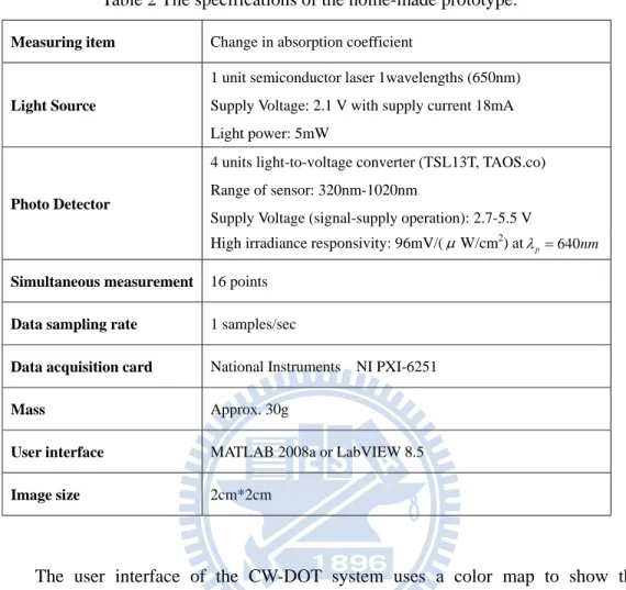
The user interface of the CW-DOT system uses a color map to show the distribution of change in absorption coefficients in different points and the system supply reasonable spatial and high temporal resolution to be scanned.

1.4 Scope and contributions of this research

DOT is developing rapidly and becoming more and more important lately. There are also more and more researches about clinical applications of DOT. For these reasons, this research aims to reduce the bulk of DOT system and lessen the computation overhead of image reconstruction algorithm in order to implement DOT on portable devise with VLSI.

At first, the homemade prototype of CW-DOT system was built to emulate the real value of detectors. Figure 1.5 demonstrates the prototype. The user interface

Table 2 The specifications of the home-made prototype.

Measuring item Change in absorption coefficient

Light Source

1 unit semiconductor laser 1wavelengths (650nm) Supply Voltage: 2.1 V with supply current 18mA Light power: 5mW

Photo Detector

4 units light-to-voltage converter (TSL13T, TAOS.co) Range of sensor: 320nm-1020nm

Supply Voltage (signal-supply operation): 2.7-5.5 V High irradiance responsivity: 96mV/(μW/cm2_{) at}

640

p nm

λ =

Simultaneous measurement 16 points

Data sampling rate 1 samples/sec

Data acquisition card National Instruments NI PXI-6251

Mass Approx. 30g

User interface MATLAB 2008a or LabVIEW 8.5

made real-t suppl card P I with     Figu CW NI P e by LabVIE time. Figure ly card whic PXI-6251 is In emulation concentrated             ure 1.5 Over W-DOT system PXI system. EW which (b) is a set ch can config shown in fi n, the glue an d hemoglobi (a)          (c)   rview of the m. (b) A set (d) FPGA p is in (a) an t of sensor n gure the DC gure (c). Th nd blood of in. The glue           proposed CW of sensor ne platform. (E) nd it can sh networks. NI C voltage and e last figure

pig were use e is the homo             (E) W-DOT syst etworks. (c) ) The flow of

how the rec I PXI system d current an

(E) is the flo

ed to emulat ogenous me       (b

  (

tem. (a) Use Power suppl f emulation. construction m included t nd the data a ow of emula te the biolog edium while b)  (d)  er Interface o ly and DAQ image in the power acquisition ation. ical tissue the blood     of Q card of

is the inhomogenous medium with bigger absorption coefficient. The result of image reconstruction displays the allocation of inhomogenous medium is as same as the site of blood. The result proves the accurate of the reconstruction algorithm.

The second part of this research is studying image reconstruction algorithm with intend to reduce its complexity. Various models of biological tissue and reconstruction modes are simulated. Eventually, the algorithm of inverse solution is chosen and realized by hardware description language (HDL) with appropriate design methodology in order to adapt to portable instrumentation.

There are three chapters in the essay. Chapter 1 is the introduction of various medical imaging techniques and background of this research. The theories, techniques, and relative application of DOT and NIRS are interpreted in chapter 2. In chapter 3, the algorithms of image reconstruction and the results of simulations are shown. Moreover the design of hardware architecture and specifications of image reconstruction processor are demonstrated.

Chapter 2 Diffuse Optical Medical Imaging Technique

2.1 Photon migration

When photons travel through a medium, they are affected by two factors which are scattering and absorption. Scattering is caused by collusion with molecules in the medium and the characteristics and direction of photons will be changed after scattering. Decreasing of light intensity or disappearance of photons are called absorption. Scattering coefficient and absorption coefficient can be used to quantify these abilities of different mediums.

If a medium is composed of various substances with no order, it can be view as “turbid medium”, which have relative large scattering coefficient. The most common turbid medium is biological tissues. The components biological tissues are lipid, water, hemoglobin and others. While a light incident into a turbid medium, it meets a large possibility to be scattered and its frequency, polarization, and travel path are changed disorderly.

Nevertheless, the paths of the photons still can be divided into three main groups shown in Fig. 2.1 [12]. Few photons go through the turbid medium directly without any scattering are “ballistic photons” and these photons contain the most information of the original photons. CT systems use these ballistic photons to construct image. Some photons diffuse through the same direction and company with some scattering condition are “snake photons”. When a light incidents into the turbid medium, most photos belong “diffusion photons” after they undergo huge amount of scattering and also absorption during pass through the tissue. A part of diffusion photons transfer out of the same surface as they enter in or pass through the tissue. That is the reason you can see some light is going into several centimeters in your hand when you shine a laser light onto your hand.

Although, the original attributes of diffusion photons have been changed by scattering, the big amount of these photons still has useful messages after they pass through the tissue. For instance, the absorption ability or components of the biological tissue affect the density of diffuse reflection.

Therefore, if there is more detectable diffusion photons get out of tissue, there is more opportunity to construct the characteristics of the tissue. The light source is chosen by acquiring the absorption coefficient of three main absorbers of human tissue within different wavelengths light. The spectrum is demonstrated in Fig. 2.2

  Figure 2.1 Different types of travel paths of photon migration [12]

 

In figure 2.2, we can found that HbR, HbO2 are relatively weak absorbers at

near-infrared wavelengths. This characteristic allows the photons of near-infrared ray (NIR) to penetrate through the tissue deeper and still can be detected. The range of the wavelengths is also called an “optical window” of biological tissue[12]. The spectrum of HbO and Hb are distinct enough to permit us recognize the difference within the window.

According to the usage of NIR, NIR spectroscope (NIRS), NIR imaging (NIRI) and diffuse optical tomography (DOT) are the main applications. NIRS is a way to measure the concentration of HbO2 and Hb by detecting the diffusion photons. While

NIRS can quantify the whole situation of an area, it lack of depth or location information. DOT uses more complicated algorithm to construct features of medium and the spatial resolution is higher than NIRS. DOT employs multi optical sources and detectors to reconstruct 2-D and 3-D images of biological tissue. More specific principles and applications of NIRS and DOT are introduced later.

2.2. Near-Infrared Ray Spectroscope

Near Infrared Spectroscopy (NIRS) use two or more than two various optical wavelengths to compare the absorption property of different components in biological tissue. NIRS system measures the light and electricity signal so it can reveal the change of tissue quickly. This section presents the theory and applications of NIRS.

2.2.1. Modified Beer-Lambert Law

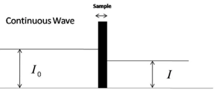
In high turbid medium such as human tissue, Modified Beer-Lambert Law is usually used to describe the result of the optical density after a light migrates through the medium [13]. It is written as Eq. (1).

Optical density attenuation log out in

I

OD A S

I λ λ

= = − = + (1)

density after the light penetrating through the biological tissue. The quantity of optical density attenuation isOD and it is referred as the superposition of absorption Aλ

and scattering S_λ quantities which are the main factors to weaken the light. The absorption part of attenuation can be formulated as Eq. (2).

2 , , i i i Hb HbO A_λ ε _λC L_λ = =

∑

(2)

Theε_i,λ is specific extinction coefficient of different absorbers and optical

wavelengths. Ci are the concentrations of blood chromophores which are the main

absorber. Figure 2.3 shows the one channel NIRS system and the diffusion photons pass from source to detector form the “banana shape”.

The Lλ is the total length of the radiation go through the biological tissue which

relate to the distance of the source and detector d and the differential path-length fa DPF_λ. DPF_λ is composed with the absorption coefficient and reduce scattering

coefficient. Due to the anisotropy of the scattering property, reduce scattering coefficient replace scattering coefficient. The total path of the radiation can be written as Eq. (4) and the DPF_λ is demonstrated in Eq. (5).

Lλ = ⋅d DPFλ (4)

  Figure 2.3 One channel NIRS system. [13]

1 ' 2 , 1 ' , 2 , , 3 1 1 1 2 1 (3 ) s a s a DPF d λ λ λ λ λ

μ

μ

_{μ μ}

⎡ ⎤ ⎛ _{⎞ ⎢ ⎥} = ⎜_{⎜ ⎟ ⎢⎟} − _⎥ ⎝ ⎠ _{⎢⎣ + i ⎥⎦} (5)

The S_λ in Eq. (3) is the attenuation which is caused by scattering. The

scattering coefficient and geometry of the tissue influence S_λso it is unknown and too complex to measured. But it can viewed as constant in same medium so we can get the change of chromophores concentration by measure the attenuation of the optical density. After successive measurement of light density we can obtain different light attenuation. The formula can be written as Eq. (6).

,final ,initial i, i

ODλ ODλ ODλ ε λ C dDPFλ

Δ = − =

∑

Δ (6)

In human tissue, water and lipid are weak absorbers within optical window so its concentration could be viewed as constant and ignored. Getting the changes of concentration of HbO and Hb are the main applications of NIRS. In order to obtain these two values, two different wavelengths which are over and below 800nm optical sources are need generally. Therefore, the Eq. (6) can be written as Eq. (7).   

Finally, the change of chromophores concentration can be obtained from Eq. (9).  

1 2 2 , , HbO Hb OD C OD M C OD C OD C λ λ Δ Δ ⎡ ⎤ ⎡ ⎤ Δ = ×Δ Δ =⎢_Δ ⎥ Δ =⎢_Δ ⎥ ⎢ ⎥ ⎣ ⎦ ⎣ ⎦ (7) 2 1 2 2 1 1 2 2 , , , , 0 0 T HbO HbO Hb Hb DPF M d DPF λ λ λ λ λ λ

ε

ε

ε

ε

⎛⎡ ⎤ ⎡ ⎤⎞ = ⎜_⎜⎢ ⎥ ⎢× ⎥⎟_⎟ ⎢ ⎥ ⎢ ⎥ ⎣ ⎦ ⎣ ⎦ ⎝ ⎠ (8) 1 C M− OD Δ = × Δ (9)

2.2.2 Application and implementation of NIRS

By Modified Beer-Lambert Law, NIRS provide the real-time measurement of chromophore. There are some applications by measuring the concentration of chromophores. Using blood chromophores concentration, oxygenation and blood

volume changes in tissue such as Eq. (8) and Eq. (9) can be defined. 2 HbO Hb OXY = ΔC − ΔC (9) 2 HbO Hb BV = ΔC + ΔC (10)

The OXY and BV are estimates proportional to the change of oxygenation and blood volume. By observing these values, testing screen testing of infant can be realized [13]. NIRS can also be used to exam the function of brain and called functional NIR (fNIR)[14][15]. NIRS is also applied on diagnosing cancer base on the difference of endogenous chromophore between anomaly and normal tissues [15]. The breast tumor is the main part of exam.

The NIRS has been developed for several decades, and there are some different modalities to implement NIRS. In the way of time-domain modality, high speed about picoseconds pulsed laser and time resolve measurements were used so it has high resolution. But the heavy instrument let the investigators proposed RF system. The RF system modulates laser diodes and detectors the phase delay and the amplitude of modulated light.

The other newer application is NIR image (NIRI). It has gained interest to researchers recent years. NIRI can be referred as the extension of NIRS with multi-channel of source and detectors. The result of concentration image of chromophores is showed by color mapping.

2.3. Diffuse Optical Tomography

We have known that the main absorber in biological tissue is HbO2 and Hb.

Therefore, the optical characteristics of absorption or scattering ability are affected by chromophores. The DOT uses another algorithm to approach the optical characters of tissue. In order to generate a mapping image of spatial variations optical parameters, we need to measure the photon fluence with multiple sources and allocate detectors to

back-project the image essentially. This section introduces the theory and approach ways of DOT system.

2.3.1 Diffuse equation

To describe how the near-infrared photon migration through biological tissue has been developed based on the radiative transfer equation (RTE) about the 1990s. The scattering probability is much greater than absorption probability in turbid medium. Therefore diffusion approximation to the transport equation can be used. The diffusion equation is showed as Eq. (6).

2 _{( , ) ( , ) ( , ) ( , )} a D r t r t r t S r t t νμ ∂ ν − ∇ Φ + Φ + Φ = ∂ (11)

The Φ( , )r t is the photon fluence at position r and at time t. S r t( , ) is the light intensity of the light source. D is the scattering factor which distinct from the optical characteristics and can be presented as Eq. (11).

' ' 3 s a 3 s D

ν

ν

μ αμ

μ

= ≅ + (12)

The μ_s'and

μ

_a are reduce scattering and absorption coefficient of objective. In turbid medium,

μ

_s' much greater than

μ

_a so D can be reduced to the right side of Eq. (11). The optical properties of biological tissue can be found in reference [16].

ν

is light speed of the medium. Note that the parameters in Eq. (11) are dependency to wavelength of light source. The relation between μ_a and concentration of HbO2 and

Hb is showed in Eq. (12).

2, [ 2] , [ ]

a HbO λ HbO Hbλ Hb

μ

=

ε

+

ε

(13)

To get the variation of absorption coefficient the Φ( , )r t should be measure first. Eq. (11) is an implicit equation and it demand to do the approximation and linearization to simplify the diffusion equation.

early tumor detection, brain function image, and early discrimination between ischemic and hemorrhagic stroke. There are several technical solutions to realize DOT system, including time domain (TD), frequency domain (FD), and continuous wave (CW) techniques.

2.3.2 Application and implementation of DOT

TD-DOT use ultra high speed laser (picoseconds) to incident pulses of light into the tissue. After the pulses incident the tissue, various tissue made them board and attenuate which is mean reshape the pulse. TD system detects amplitude and temporal distribution when they penetrate out of the surface of tissue. In figure 2.4, the head of the long pulse is the photons which don’t undergo many scattering effect and are called ballistic photon. While the photons reach the detectors slower they also contain more information about the depth, optical characteristic and others. TD systems have some advantage, the scattering coefficient of tissue can be get by calculate the slope of the long pulse and TD-DOT also have relatively high spatial resolution to FD-DOT and CW-DOT.

On other hand, TD systems are very expensive, large dimension and long acquisition times to receive reasonable signal- to-noise ration. The high speed optical detectors are also needed to implement the systems such as streak camera, avalanche photon-diode and photomultiplier.

  Figure 2.4 The modality of TD-DOT systems.

In FD systems, amplitude of optical sources are modulated at frequency about tens to hundreds megahertz which is between TD and CW systems. This system reconstruct the information of tissue by detect the amplitude decline and the phase delay of the photon. After modulating, the light includes AC and DC component. The AC part has phase and the amplitude component and the DC part also has the information of amplitude. Fig. 2.5 shows the modality of FD-DOT system. The phase delay is hard to detect because of modulate of the optical sources. Therefore, when the signals are detected, the cross-correlation also is done at the same time. The frequency of signal is modulated to below 1 kHz to obtain the ration of AC and DC amplitude and the phase delay.

Compare to TD system the photon penetrate depth of FD system is shallow, but temporal revolution is much higher than TD systems. The optical source of CW-DOT system is very low frequency and steady compare to “pulse” in TD systems. The optical sources can view as on continuously. The information obtains from optodes is only the DC amplitude so scattering parameter can’t obtain in CW systems. Scattering coefficient is usually set to be constant in CW-DOT. The reconstruction algorithm is relative simple and computation overhead is lower than other two systems.

  Figure 2.5 The modality of FD-DOT systems.

The main characteristics of CW-DOT systems are the high potential to achieve the goals of low-power, low-cost and portable. The optical sources and detectors have less criteria and easy to assemble. The power consumption of CW is lower which 3.6V Li-ion battery can drive. So, CW-DOT systems have the highest potential to commercialize and massive produce. The relatively poor penetration and localization are the shortcoming of CW-DOT systems. The ability to precise the localization is influenced by the power of optical sources, the sensitivity of sensors and the reconstruction method. How to tradeoff between spatial resolution and makes it portable is a challenge. Table 3 reveals the pros and cons of different systems.

  Figure 2.6 The modality of CW-DOT systems.

Table 3 Pros and cons of different types of DOT systems. 

Type Advantages Disadvantages

TD 1. Spatial resolution 2. Penetration depth

3. Most accurate separation of absorption and scattering

1. High Sampling rate 2. Instrument size and weight 3. Stabilization and cooling 4. Cost

Example Uses: Imaging cerebral oxygenation and hemorrhage in neonates, breast imaging. FD 1. Relatively low sampling rate

2. Relatively accurate separation of absorption and scattering

1. Penetration depth

2. Instrument size and weight 3. Cost

Example Uses: Cerebral and muscle oximetry, breast imaging CW 1. Low sampling rate

2. Instrument size, weight and simplicity 3. Low cost

1. Penetration depth

2. Difficult to separate absorption and scattering.

2.4. Review of this study and Recent Work

NIRS and DOT both use the “optical window” to obtain the message from biomedical tissue. But there are some difference between NIRS and DOT. The most significant difference is the algorithm the two system use. NIRS system can get the absolute value of chromophores concentration by modified Lambert Law. DOT use the diffusion equation to calculate the change and absolute value of optical coefficient. NIRS can also be showed as image such as the distribution of Hb concentration.

The relevant researches about NIRS and DOT have been undergone for decades. In 1929, using continuous wave (CW) light to detect breast lesions was first proposed by Cutler. But the light intensity is too high to heat the patient. In 1973, Gros et al. used near-infrared ray and allocated the breast between physician and optical source. The Doctor uses eye to see the “image” directly. As times goes on, the newer technology was developed. The below table presents the relevant research with some figures of instrument in recent years.

  (a) (b)

Figure 2.7 (a) Schematic drawing of a high-speed laser Doppler blood flow imager. (b) Blood flow-related images of human fingers. Images size is 512x512.

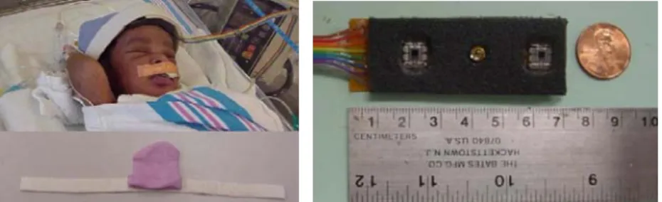
Recently, how to enhance the spatial resolution and the portability of instrument are hot issues. The forward model, inverse solutions, sensor network, and front-end circuits are the some causes to affect the quality and volume of imaging systems. Portable instrument for bedside monitoring of newborn brain have proposed which is showed in Fig. 2.9. There are also some commercial topography products such as

 

(a) (b)

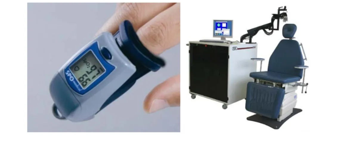
Figure 2.8 (a) Pulse Oximetry (b) CW-DOT system of NIRx company. Table 4 Relative researches about NIRS and DOT.

Item description From

Pulse Oximetry (Figure 2.8a)

Provide accurate oxygen saturation of arterial. 1930s

Laser Doppler Blood Flowmetry

(Figure 2.7)

Measure in-vivo blood flow in biological tissues such as skin or brain tissue by measure the beam of the reflected light.

1960s

Near Infrared Spectroscopy (NIRS)

Quantifies changes in chromophore concentration in turbid medium by measure the change in the photon density of light.

1970s

Phonon Migration Instrumentation

An extension of an NIRS system but it has more sources and detectors. There are three kinds of system to implement it: a. Use pico-second pulses of light

b. Continuous wave illumination c. RF amplitude modulated illumination

1980s

Diffuse Optical Tomography (DOT)

(Figure 2.8b)

Estimate the optical parameters of the biomedical tissue by invert the photon propagation model. Also three ways to approach: TD-DOT , FD-DOT , and CW-DOT.

Hitachi ETG-7100 in Fig. 2.8 (b) and NIRx Scout and Fig. 2.10. Because the computation workstation is heavy, the volumes of these systems are not suitable to portable applications.

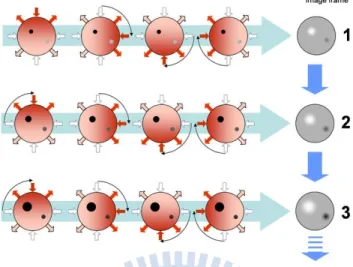
The other method of DOT is dynamic near-infrared optical tomography (DYNOT) which developed by optical tomography group of SUNY Downstate Medical Center. DYDOT employs low-energetic laser radiation to probe tissue. The multiple optical sensors acquire data set in a continuous fashion at high repetition rates about several images per second [17]. So the study of physiologic changes inside the target can be scan. The concept is illustrated in the figure below. DYDOT is apply on scan breast mainly, because the tissue of breast is relative simple to brain and the depth of penetration of light is deeper.

Algouth there are lots of instrument have been developed, an portable DOT tomograpghy system instrument with the reconstruction compute system which can be applied the on urgent diagosis and wearble are not implemented. Next section the

   

Figure 2.9 (a) Sensor attached on the hat. (b) LED and photo-diode.

  Figure 2.10 (a) Hitachi ETG-7100 (b) Array of sensor network

method of the VLSI inspired image reconstrction algorithm and the design of processor is illustrated and show the result of simulations.

 

Figure 2.11 Concept of DYNOT. The input arrows indicate the direction of light. (Source: http://www.nirx.net/dynamic-optical-tomography)

Chapter 3 Image Reconstruction Algorithm and Processor

To reconstruct the topography of tissue the forward model and inverse solution are two critical processes. Forward model is employed to describe how the photons scatter and diffuse in highly scattering medium. The optical density sense by the detectors can be expected and calculated from forward model. Inverse solution is used to reconstruct optical characteristics of the medium with the modalities of detectors.

3.1 Forward Model

The diffusion equation is a standard approach in high scattering medium. For the using of continuous optical source, the Eq. (11) in chapter 2 can be expressed as Eq. (14)

2

( ) _a ( ) ( ) D r

υμ

r

υ

S r

− ∇ Φ + Φ = (14)

To solve the equation, the most common techniques of linearization are Born and the Rytov approximations [5][18]. The main difference of these approximations is the assumption of light intensity Φ( )r _{at position} r. Born technique approximates the light intensity is superposition of incident component and scattering component which is showed in Eq. (15). The hypothesis of Born is based on the intensity of incident light much bigger than scattering. Therefore when the variation of absorption coefficient reaches a quantity the method is not adapted to be used. In Rytov approximation, there is a nature exponential relation of incident light and scattering light in Eq. (16) and the method is suit for the reasonable change of absorption. Born approximation has been proven it leads much more ill-posed than the Rytov approximation thus Rytov approximation is used to do simulation in the study.

( )r _incident( , )r r_{s scat}( , )r r_s

Φ = Φ + Φ (15)

( )r _incident( , ) expr r_{s scat}( , )r r_s

To get the change of absorption coefficient, the μ_acan be express as Eq. (10). We assume that the object is a homogenous medium with constant absorption coefficient μ_ah and heterogeneous mediums in homogenous medium cause the variation of absorption coefficient Δ .[19] μ_a

h

a a a

μ =μ + Δμ (17)

Next, apply Eq. (16) and Eq. (17) to Eq. (14); the Eq. (18) can be obtained.

(

)

( )

( )

( )

2 , exp , h a a incident r rs scat r rs S r D

ν μ

μ

ν

⎛_{∇ − + Δ} ⎞_{Φ Φ =} ⎜ ⎟ ⎝ ⎠ (18)

The incident Helmholtz equation which with no scattering and variation of absorption is represented as Eq. (12).

( )

( )

2 , h a incident r rs S r D

ν μ

ν

⎛_{∇ −} ⎞_{Φ =} ⎜ ⎟ ⎝ ⎠ (19)

To solve the Δμ_a we use Eq. (18) to subtract Eq. (19) and get the Eq. (20).

(

2 2

)

(

( )

( )

( )

)

( )

( )

( )

exp a exp

inci scat in in scat

r

k r r r r r

D

ν μ

Δ

∇ + Φ Φ − Φ = − Φ Φ (20)

By using the appropriate green function and using the hypothesis of Rytov approximation: the strength change of scattering is very slowly. The scattering intensity can be expressed as Eq. (21).

1 ( , ) ( , ) ( , ) ( , ) a scat s d _v s d in s d r r r r G r r dr r r D

ν μ

Δ Φ = − Φ Φ

∫

(21)

We have defined the change of light intensity from source to detector in Eq. (22). The Eq. (21) is the integral of volume. If the volume is divided into tiny voxel we can rewrite the equation as Eq. (23).

(

)

(

)

(

)

, In , , s d scat s d in s d r r OD r r r r Φ = − = Φ Φ (22)

(

_,

)

_{( , )}

₍

( , )

₎

_{( , )} 3 , n i a scat s d i s i i i d i in s d OD r r r r G r r l D r r ν μΔ = Φ = Φ Φ

∑

(23)

The i is the number of the voxel and l is the side-length of each voxel. Eq. (23) can be expended to multiple source-detector pairs. If a system include i sources and j detectors we can receive the m= × values of the change of light intensity. The i j equation can be expressed as matrices in Eq. (24).

( ,1) 1 1 _{11 12 1 1} ( ,2) 1 2 21 22 2 2 1 ( , ) ( , ) _{( )} ( , ) ( ) ( ) ( , ) scat s d _{n a} scat s d n a m mn a n scat m si dj r r _{a a a r} r r a a a r a a r r r μ μ μ Φ ⎡ ⎤ ⎡ ⎤⎡Δ ⎤ ⎢_Φ ⎥ _{⎢ ⎥⎢Δ ⎥} ⎢ ⎥_{=⎢ ⎥⎢ ⎥} ⎢ ⎥ _{⎢ ⎥⎢ ⎥} ⎢ ⎥ ⎢ ⎥⎢_Δ ⎥ Φ ⎢ ⎥ ⎣ ⎦ ⎣ ⎦ ⎣ ⎦ (24)

The element a_mn of the Eq. (25) is weighting function in different locations can

be derive from Eq. (23). Δμ_a( )r_n represents the change of absorption coefficient of each voxel we observe.

(

)

3 ( , ) ( , ) ( , ) , n s n n n d mn in m s d r r G r r a l D r r

ν

Φ = Φ (25)

By linearizing the forward model, the diffusion equation can be express as Eq. (26). If we can solve the pseudo inverse of the matrixA_{m n×} , the variation of absorption

coefficient can be obtained. The processing of calculating the pseudo inverse is called inverse solution.

[ ]

Ψ m×1=

[ ]

A m n× × Δ

[ ]

μ n×1 (26)

[ ]

[ ]

†

[ ]

1 1 n A n m m

μ

_{× × ×} Δ = × Ψ (27) 3.2 Inverse Solution

We can found that if n> in Eq. (26) which means the voxel number is bigger m than the number of source-detector pairs. At the same time, the unknown values is bigger than the equations. The inverse problem becomes the ill-posed and under-determined problem [20]. The ill-posed problem features the solution may not exist and not unique. On the other hand, forward model is a non-linear problem, but linearization is used to simplify it. The artifact distortion has been made in forward

model and the reconstruction of DOT is generally an ill-posed problem. Therefore how to choose solution of inverse problem is a crucial issue.

Because of the stable ability and reliable solution to deal with ill-posed problems, the study uses SVD to solve the inverse problem.

3.2.1 Jacobi SVD algorithm

Jacobi SVD arithmetic is a way to accomplish the calculation of SVD. It has the advantage of parallel computation and is also superior to other method to implement on VLSI[21, 22]. By the definition of SVD and Jacobi SVD, the A_{m n×} can be written

as the following form:

T T

m n m m m n n n m m m n n n m n

A _× =U _× D _× V _× →U _× A _×V_× =D _× (28)

One of the JSVD algorithms is called two-side rotation method that performs orthogonal two-side plane rotations to generate matrix[23, 24]. In each rotation, the pairs of set( , )p q of matrix A_{m n×} is performed 2-by-2 SVD to generate Jl( , , )p q θ and Jr( , , )p q φ by CORDIC (COordinate Rotation Digital Computer) algorithm. The procedure is showed in Eq. (22) and Eq. (23).

1

2 0

cos sin cos sin

0

sin cos sin cos

T pp pq qp qq a a a a σ θ θ φ φ σ θ θ φ φ ⎡ ⎤ ⎡ ⎤ ⎡ ⎤ ⎡ ⎤ = ⎢ ⎥ ⎢ ⎥ ⎢₋ ⎥ ⎢₋ ⎥ ⎣ ⎦ ⎣ ⎦⎣ ⎦ ⎣ ⎦ (22) 1 0 0 0 0 cos sin 0 ( , , ) ,( ) 0 sin cos 0 0 0 0 1 pp pq qp qq J p q p q θ θ θ θ θ ⎡ ⎤ ⎢ ⎥ ⎢ ⎥ ⎢ ⎥ ⎢ ⎥ =_{⎢ ⎥} < ⎢ ₋ ⎥ ⎢ ⎥ ⎢ ⎥ ⎢ ⎥ ⎣ ⎦ (23)

Every iterative procedure makes the result more diagonal than former. After i

The equation of rotation is shown in (24).

1 0 0 0 1

( l T) ( l ) ...(T l T) r ... r r

i i i i i

D= A = J J₋ J A J J₋ J (24)

CORDIC is an iterative arithmetic and introduced in 1959 by Jack E. Volder. CORDIC can compute all the trigonometric functions by vector rotation [25]. The CORDIC algorithm is derived from the general rotation transform which rotates a vector in a Cartesian plane by an angle

θ

. It can be rearranged and showed in Eq. (25). ' cos ( tan ) ' cos ( tan ) x x y y y x

θ

θ

θ

θ

= − = + (25)

To do the simplification of the Eq. (25), rotation angles are restricted to the form as tanθ = ±2−i so shift can be performed the multiplication of tangent term. Performing the series of successively smaller elementary rotations, the arbitrary angles can be obtained. The iteration form of Eq. (25) showed in Eq. (26)

1 1 ( 2 ) ( 2 ) i i i i i i i i i i i i x K x y d y K y x d − + − + = − = − i i i i (26) 1 2 1 cos(tan 2 ) , 1 1 2 i i _i i K − − d − = = = ± + (27)

The product of the K_i can be treated as a system processing gain. It approaches

0.6073 as the number of iterations goes to infinity. The angle of a composite rotation is uniquely defined by the sequence of the directions of the elementary rotations. The angle accumulator in Eq. (28) is added to CORDIC arithmetic to calculate arctangent.

1

1 tan (2 )

i

i i i

z₊ = −z di − − (28)

The CORDIC rotator is normally operated in two modes: rotation mode and vectoring mode. In rotation mode, it rotates the input vector by a specified angle. In vectoring mode, it rotates the input vector to the x axis while recording the angle required. Table 5 shows the equations of the two modes.

The two-side rotation Jacobi rotation matrices and they are generated by eliminating the off-diagonal elements of JSVD can be implemented by VLSI with the parallel way and serial way. The systolic array architecture or the look-up table architecture can realizes the algorithm.

3.2.2 Truncated SVD

Truncated Singular Value Decomposition (TSVD) algorithm is a way to retains the t numbers of biggest non-zero singular values which is shown in Eq. (29)[10]. The

t is referred as the truncated parameter. The computation can be reduced by adding the truncated operations, because the rest of diagonal elements of can be set to zero. At the same time, not all of the singular values are important. TSVD can also be helpful to simplify the computation complex.

1 0 0 0 0 0 0 0 0 0 0 0 0 0 0 0 0 0 0 0 0 0 0 T m n m m t n n m n A U V σ σ × × × × ⎡ ⎤ ⎢ ⎥ ⎢ ⎥ ⎢ ⎥ = ⎢ ⎥ ⎢ ⎥ ⎢ ⎥ ⎣ ⎦ (29) Table 5 The two modes of CORDIC.

Rotation Mode Vectoring Mode

Input vector 1 1 1 1 2 2 tan (2 ) i i i i i i i i i i i i i i x x y d y y x d z z d − + − + − − + = − = − = − i i i i i where 1 if 0, 1 otherwise i i d = − z < + 1 1 1 1 2 2 tan (2 ) i i i i i i i i i i i i i i x x y d y y x d z z d − + − + − − + = − = − = − i i i i i where 1 if y 0, 1 otherwise i i d = − < + Result 0 0 0 0 0 0 2 [ cos sin ] [ cos sin ] 0 1 2 n n n n n i n n x A x z y z y A y z x z z A − = − = + = =

∏

+ 0 0 0 1 0 0 0 2 [ cos sin ] 0 tan ( / ) 1 2 n n n n i n n x A x z y z y z z y x A − − = − = = + =

∏

+

3.2.3 Frame mode and sub-frame mode of image reconstruction

Two modes of inverse operations are proposed: one is called the frame mode and the other is called the sub-frame mode. We define a frame contains 96 voxel within an area of _{(4 6)cm}× 2_{. In the frame mode, an image with 96 voxel is reconstructed} directly. Thus, there are totally 96 numbers of Δ have to be solved in one system μ_a of linear equations. The biggest truncated number is 72 in the frame mode and the size of matrix Frame

A is 72 96× . In the sub-frame mode, a frame is divided into six sub-frames with

4 4

×

voxel, thus the dimension of matrix

A

can be reduced significantly. The biggest truncated number is 4 _{and the matrix size of} ASub Frame− is

4 16× . By this way, six much smaller inverse problems are solved instead of solving one big problem. Simulation results of two modes are presented in next section. Fig. 3.1 displays the relation between sub-frames and one frame.

3.3 The result of software simulation and analysis

Figure 3.2 is the simulation flow chart of simulation. MATLAB is used to handle the simulation. First, the geometry of sample is defined by the medium size and the locations of the source-detector pairs. Totally six diffuse optical sources and twelve photo-detectors are located and it demonstrated in figure 3.3. The area of frame is 4cm×6cmand the voxel size is (0.25cm)3. Second, the medium optical coefficients

  Figure 3.1 The relation between sub-frames and one frame.

are assigned to each voxel. The background medium is homogenous with 1

0.05

h a

cm

μ

₌

−

and the reduced scattering coefficient

μ

_s'

=

10

cm

−1.

  Figure 3.3 The distribution of sources and detectors.

 

T surfa Anom a

μ

simul appro T param tolera also m 0.01 in the Fi Two kinds o ce. In fi 1

0.21

maly

cm

=

lated optica oximation fo To initialize meter should ance parame means incre in two diffe e sub-frame Figure 3.4 T igure 3.5 (a) f inhomogen gure 3.4 1

m

− and lef l density m orward mode e the invers d be set. In eter can lead easing the c erent modes. mode and 6, Two inhomog me Frame mod neous media the right-ft-side medi measurements el. e resolution some cases, d to higher q omputationa . The trunca , 12, 18, or 2 geneous med edium. (b) T 10 de with t=18. a are embed -side inhom ium is with s on the sur n, the trunca , a bigger tr quality of im al cost. The ated paramet 24 in the fram dium with d The second m 0-2 . Figure 3 ded at depth mogeneous h

μ

aAnomaly2

=

rface are ob ated parame runcated par mage. Nevert tolerance p ter t is assign me mode. different loca medium. 3.6 (a) Sub-F h of 0.5 cm medium 1

0.5cm

−

=

. T btained by t

eter and the rameter and theless, high parameter is

ned to be 1, ation. (a) The

Frame mode below the is with Then, the the Rytov tolerance a smaller her quality set to be 2, 3, or 4 e first 10-2 with t=3. 10-2

F numb first m I The r evalu Fig   Fig Fig Figure 3.5 ( bers and figu

medium.

In second m results of im uate the qual

gure 3.5 (b) gure 3.7 (a) F gure 3.7 (b) F (a-b) show t ure 3.6(a-b) medium, we mage reconst ity and comp Frame mode

Frame mode

Frame mode

the result o are the resu

locate all th truction are p putation ove e with t=24. with t=6. e with t=12. of using fram lt of using s he inhomoge presented in erhead of the Figure 3.6 Figure 3.8 Figure 3.8 me mode w ub-frame m eneous tissue n figure 3.7(a e modes reco 6 (b) Sub-Fra 8 (a) Sub-Fr (b) Sub-Fra with various mode to recon es within su a-b) and 3.8 onstruction i ame mode w rame mode w ame mode w truncated nstruct the ub-frames. 8 (a-b). To image, the with t=4 10-2   with t=1   with t=2. 10-2 10-2