於時間相關通道下之雙模式有限回授傳送波束形成技術

(1)

國立交通大學

電信工程學系碩士班

碩士論文

於時間相關通道下之

雙模式有限回授傳送波束形成技術

Transmit Beamforming with Dual-Mode Limited

Feedback over Temporally-Correlated Channels

研究生：陳亮元 Student:

Liang-Yuan

Chen

指導教授：李大嵩博士 Advisor:

Dr.

Ta-Sung

Lee

(2)

於時間相關通道下之

雙模式有限回授傳送波束形成技術

Transmit Beamforming with Dual-Mode Limited

Feedback over Temporally-Correlated Channels

研究生：陳亮元 Student: Liang-Yuan Chen

指導教授：李大嵩博士 Advisor:

Dr. Ta-Sung Lee

國立交通大學

電信工程學系碩士班

碩士論文

A Thesis

Submitted to Institute of Communication Engineering

College of Electrical and Computer Engineering

National Chiao Tung University

in Partial Fulfillment of the Requirements

for the Degree of

Master of Science

in

Communication Engineering

June 2007

Hsinchu, Taiwan, Republic of China

(3)

於時間相關通道下之

雙模式有限回授傳送波束形成技術

學生：陳亮元

指導教授：李大嵩博士

國立交通大學電信工程學系碩士班

摘要

在新一代無線通訊中，有限回授前置編碼（Limited Feedback Precoding）為一用以提升系統可靠度的技術，其特色在由接收機回傳最佳前置編碼的編號給發射機，且發射機不需要任何的通道狀態資訊。在本論文中，吾人主要探討在多輸入單輸出（Multiple-Input Single-Output, MISO）系統中的傳送波束形成技術（Transmit Beamforming）；傳統的作法，在固定平均回授率的情況下，單一模式有限回授系統（只有一個編碼簿）在時變通道下並不夠強健。假設接收端有完整的通道狀態資訊、無錯誤的回授通道，和一階馬可夫多輸入單輸出通道模型，吾人提出一個雙模式有限回授系統和基於符元錯誤率的模式選擇準則，在連續的兩個單位時間內，考慮兩種傳送波束形成模式：（1）在每個獨立的單位時間內，用較小容量的編碼簿個別作波束形成；（2）在兩個單位時間內，用較大容量的編碼簿聯合作波束形成。利用連續兩個單位時間內的時間相關係數和完整的通道狀態資訊，吾人提出的模式選擇準則，可以選擇較佳的模式傳輸。由模擬結果可以看出雙模式有限回授前置編碼系統效能優於單模式有限回授前置編碼系統。

(4)

Transmit Beamforming with Dual-Mode Limited

Feedback over Temporally-Correlated Channels

Student:

Liang-Yuan

Chen Advisor:

Dr.

Ta-Sung

Lee

Department of Communication Engineering

National Chiao Tung University

Abstract

Limited feedback precoding is a technique used to improve system reliability in modern wireless communications. The feature of limited feedback precoding is that receiver feeds back the index of the optimal precoder to the transmitter. The transmitter does not need to have any channel state information (CSI). In this thesis, we focus on the transmit beamforming scheme in multiple-input single-output (MISO) systems. In conventional approach, under a fixed average feedback rate, the single-mode limited feedback system (has only one codebook) is not robust enough in time-varying channels. Perfect channel knowledge known at the receiver, error-free feedback channel, and first-order Markov MISO channel model are assumed in this thesis. We propose a dual-mode limited feedback system with a symbol-error-rate (SER) based mode selection criterion. Two transmit beamforming modes over two consecutive time slots are considered: (1) separate beamforming for the individual time slot with a small-size codebook, and (2) joint beamforming for both slots with a large-size codebook. By exploiting the temporal-correlation coefficient of two consecutive time slots and perfect channel knowledge, the better mode can be selected by using the mode selection criterion. Simulation results show that the performance of the dual-mode limited feedback system is better than that of the single-mode limited feedback system.

(5)

Acknowledgement

I would like to express my deepest gratitude to my advisor, Dr. Ta-Sung Lee, for his enthusiastic guidance and great patience. I learn a lot from his positive attitude in many areas. Heartfelt thanks are also offered to all members in the Communication System Design and Signal Processing (CSDSP) Lab for their constant encouragement. Finally, I would like to show my sincere thanks to my parents for their invaluable love.

(6)

Chinese Abstract

I

English Abstract

II

Acknowledgement III

Contents IV

List of Figures

VI

List of Tables

IX

Acronym Glossary

X

Notations XI

Chapter 1 Introduction... 1

Chapter 2 Limited Feedback Precoding for MIMO Systems ... 4

2.1 Limited Feedback Systems ... 5

2.1.1 Limited Feedback MIMO Channel Model ... 5

2.1.2 Decoding Scheme of Limited Feedback MIMO Systems ... 7

2.2 Precoder Selection Criteria ... 9

2.2.1 Capacity Selection Criterion ... 9

(7)

2.2.3 Minimum Singular Value Selection Criterion... 10

2.3 Codebooks for MIMO Precoding Scheme in IEEE 802.16-2005 ... 12

2.4 Summary ... 15

Chapter 3 Single-Mode Limited Feedback Precoding for MISO

Systems... 16

3.1 Single-Mode Limited Feedback Systems ... 17

3.1.1 First-Order Markov MISO Channel Model ... 18

3.1.2 Decoding Scheme of Limited Feedback MISO Systems... 20

3.2 Transmit Beamforming Codebooks in IEEE 802.16-2005 ... 21

3.3 Computer Simulations ... 26

3.4 Summary ... 39

Chapter 4 Dual-Mode Limited Feedback Precoding for MISO

Systems... 40

4.1 Dual-Mode Limited Feedback Systems... 41

4.2 SER Based Mode Selection Criterion for MISO Systems... 43

4.3 SER Based Mode Selection Criterion for MISO-OFDM Systems... 55

4.3.1 Review of OFDM ... 55

4.3.2 Multipath First-Order Markov MISO Channel Model ... 58

4.4 Computer Simulations ... 62

4.5 Summary ... 75

Chapter 5 Conclusion ... 76

(8)

List of Figures

Figure 2.1: Limited feedback MIMO system architecture...6

Figure 3.1: Single-mode limited feedback system architecture...17

Figure 3.2: Transmit beamforming scheme for MISO system...18

Figure 3.3: Transmit beamforming schemes of Mode I and Mode II ...26

Figure 3.4: SER performance of the single-mode 4× MISO system with 1 1 ρ = ...29

Figure 3.5: SER performance of the single-mode 4× MISO system with 1 0.9 ρ = ...30

Figure 3.8: SER performance comparison between Mode I and Mode II for 4 1× MISO system ...32

Figure 3.9: SER performance of the single-mode 4× MISO-OFDM system 1 with ρ = ...35 1 Figure 3.10: SER performance of the single-mode 4× MISO-OFDM system 1 with ρ =0.9 ...36

Figure 3.11: SER performance of the single-mode 4× MISO-OFDM system 1 with ρ =0.8 ...37

(9)

Figure 3.12: SER performance of the single-mode 4× MISO-OFDM system 1

with ρ =0.7 ...37

Figure 3.13: SER performance comparison between Mode I and Mode II for 4 1× MISO-OFDM system ...38

Figure 4.1: Dual-mode limited feedback system architecture ...41

Figure 4.2: Mode selection scheme of the dual-mode limited feedback system ...42

Figure 4.3: PDF of h_k₊₁f_k₊_1,12 with different ρ (given h and _k f_{k +}₁) ...47

Figure 4.4: SER performance of the dual-mode 4× MISO system with 1 1 ρ = ...64

Figure 4.5: SER performance of the dual-mode 4× MISO system with 1 0.9 ρ = ...65

Figure 4.8: SER performance comparison between the single-mode and the dual-mode 4× MISO systems ...67 1 Figure 4.9: SER performance comparison between the single-mode and the dual-mode 4× MISO systems with 0.71 ≤ ≤ρ 0.95 ...67

Figure 4.10: SER performance of the dual-mode 4× MISO-OFDM system 1 with ρ = ...71 1 Figure 4.11: SER performance of the dual-mode 4× MISO-OFDM system 1 with ρ =0.9 ...71

Figure 4.12: SER performance of the dual-mode 4× MISO-OFDM system 1 with ρ =0.8 ...72

(10)

Figure 4.13: SER performance of the dual-mode 4× MISO-OFDM system 1

with ρ =0.7 ...72 Figure 4.14: SER performance comparison between the single-mode and the

dual-mode 4× MISO-OFDM systems ...74 1 Figure 4.15: SER performance comparison between the single-mode and the

(11)

List of Tables

Table 2.1: MIMO precoding codebook V(2,1, 3)...12

Table 2.4: Operations to generate codebooks V N S L

(

_t, ,

)

for N =_t 2, 3, 4, 2, 3, 4 S = , and L =3, 6 ...14

Table 3.1: Transmit beamforming codebooks in IEEE 802.16-2005 standard ...21

Table 3.2: Generating parameters for V(3,1, 6) and V(4,1, 6) ...22

Table 3.4: Schemes of Mode I and Mode II for single-carrier and multi-carrier systems...27

Table 3.5: Simulation environment of the single-mode limited feedback MISO system ...28

Table 3.6: Simulation environment of the single-mode limited feedback MISO-OFDM system ...34

Table 4.1: Simulation environment of the dual-mode limited feedback MISO system ...63

Table 4.2: Simulation environment of the dual-mode limited feedback MISO-OFDM system ...69

(12)

Acronym Glossary

AWGN additive white Gaussian noise

BER bit error rate

CDF cumulative distribution function

CP cyclic prefix

CSI channel state information

DFT discrete Fourier transform

IEEE institute of electrical and electronics engineers

FFT fast Fourier transform

MIMO multiple-input multiple-output MISO multiple-input single-output MSE mean square error

MMSE minimum mean square error

OFDM orthogonal frequency division multiplexing PDF probability density function QAM quadrature amplitude modulation SER symbol error rate

SNR signal-to-noise ratio

SVD singular value decomposition

(13)

Notations

b number of bits required for the index that indicate any codeword in the codebook , j k A entry (j k of matrix A , ) s E symbol energy {}⋅ E expected value

F precoder or beamformer set k

f beamformer for the k th frame or time slot k

F precoding matrix for the k th frame or time slot k

H MIMO channel matrix for the k th frame or time slot k

i

h channel gain between the ith transmit and receive antenna for the kth frame or time slot in MISO system

L frame length ch L channel order M number of substreams FFT N FFT length CP N CP _length t

N number of transmit antennas r

N number of receive antennas

0

N noise power spectrum density M

P symbol error rate of M-QAM constellation k

n noise vector for the k th frame or time slot L

V left singular matrix of channel matrix H R

V right singular matrix of channel matrix H Λ singular value matrix of channel matrix H

R

(14)

,

k i

y received signal at the ith receive antenna for the kth frame or time slot

k frame index or time slot index

,

k i

z transmitted signal from the ith transmit antenna for the k th frame or time slot

,

k i

n additive white noise at the ith receive antenna for the k th frame or time slot 2 n σ noise power ρ temporal-correlation coefficient γ signal-to-noise ratio ( )⋅+ matrix pseudo-inverse ,mode1 k

γ average SNR over the k th frame or time slot in Mode I

,mode2

k

γ average SNR over the k th frame or time slot in Mode II

,mode1

k

SER average SER over the k th frame or time slot in Mode I

,mode2

k

SER average SER over the k th frame or time slot in Mode II

mode1

SER average SER over consecutive frames or time slots in Mode I

mode2

(15)

Equation Section 1

Chapter 1 Introduction

Wireless systems employing multiple antenna arrays at both the transmitter and receiver, known as multiple-input multiple output (MIMO) systems, promise high capacity and high-quality wireless communication links [1]. MIMO systems improve quality, capacity, and reliability. Two popular approaches for communicating in the MIMO channel are diversity and spatial multiplexing.

MIMO diversity is an approach in which information is spread across multiple transmit antennas to maximize the diversity gain in the MIMO channel. One of the popular schemes for space-time diversity coding is Alamouti scheme [2]. It provides full transmit diversity and full code rate for MIMO systems with two transmit antennas.

When channel state information (CSI) is known at the transmitter, diversity can be obtained using space-time codes (STC) [2]-[3] and transmit precoding. Transmit precoding which exploits the channel state information at the transmitter can increase various performance gains for wireless communication [4]. The design of the precoders based on different forms of the channel information available to the transmitter recently draws much attention [5]-[8]. With exact feedback of the channel state information, optimal precoders in terms of maximal channel capacity, minimal bit-error-rate (BER), and minimal symbol mean square errors were reported in [9] and [10]. Another simple

(16)

approaches used to improve the system performance are transmit beamforming and receive combining. Compared with space-time codes, transmit beamforming and receive combining achieve the same diversity order as well as additional array gain. It can significantly improve the system performance [11]-[13].

CSI known at the transmitter is not a practical assumption. Furthermore, conveying full CSI through a feedback channel is also impractical because the channel coefficients need to be quantized and fed back to the transmitter over limited bandwidth channels. Thus, limited feedback precoding schemes are proposed to solve the problem. In limited feedback precoded systems, receivers use current CSI to select the optimal precoder from a given codebook and feed back the codeword index through the limited bandwidth control channel [14]-[19]. Most of the existing works on the limited feedback precoidng focus on the development of quantization criteria and the related performance analysis. Limited feedback precoding was also mentioned in the technical reports of IEEE 802.16-2005 standard [20]-[23]. Another important issue is the optimal codebook design. Optimal codebook design is a problem of Grassmannian line packing [24]. The problem has been solved and the optimal codebooks with different dimensions and sizes are also constructed in [24]. The optimal codebooks are also considered in IEEE 802.16-2005 standard [25].

The single-mode limited feedback precoded system is a system that has only one codebook. Under a fixed average feedback rate, the single-mode limited feedback precoded system is not robust enough in mobile environments. Thus, the tradeoff problem is, “less feedback more often, or more feedback less often?”

In this thesis we study transmit beamforming with limited feedback when the channels between consecutive time slots are subject to temporal correlation. We assume that (1) two beamformer sets F and ₁ F (with, respectively, 2₂ band 22bcodewords)

(17)

are available, and (2) the average feedback rate is fixed in a transmission. We address the problem of beamforming strategy selection for two consecutive time slots. More specifically, relying on an average symbol-error-rate (SER) based criterion we wish to determine which one of the following two scheme is better: (i) separate beamforming for the individual time slot with F , (ii) joint beamforming for both slots by using ₁ F . The ₂ considered problem is motivated by the necessity of mode switching when the channels are time-varying, a scenario typically found in the mobile environment. We develop an SER based mode selection criterion for the temporal-correlation channel environment. Simulation results illustrate the advantage of the proposed method against those without mode selection.

This thesis is organized as follows. In Chapter 2, the overview of the limited feedback system and the precoder selection criteria are introduced. Moreover, MIMO precoding scheme in IEEE 802.16-2005 is also presented. In Chapter 3, single-mode limited feedback precoded system is introduced. We consider first-order Markov MISO channel model and use the codebooks defined for transmit beamforming in 802.16-2005 standard. SER performances of the single-mode limited feedback MISO system and MISO-OFDM (orthogonal frequency division multiplexing) system are also illustrated in this chapter under a fixed average feedback rate. In Chapter 4, the proposed dual-mode limited feedback systems and the SER based mode selection criterion for the temporal-correlation channel environment are presented and derived. Numerical experiments illustrate the advantage of the proposed method against those without mode selection. Finally, we conclude this thesis in Chapter 5.

(18)

Equation Section (Next)

Chapter 2 Limited Feedback Precoding for

MIMO Systems

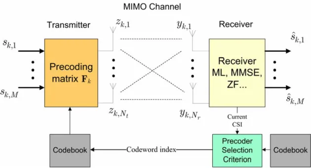
Digital communication using multiple-input multiple-output (MIMO) has recently emerged as one of the most significant technical breakthroughs in wireless communications. This technology figures on the list of recent technical advances with a chance of resolving the bottleneck of traffic capacity in future wireless communications. MIMO systems can provide high channel capacity and high reliability. When channel state information (CSI) is known at the transmitter, precoding can provide diversity gain and additional array gain. But the transmitter always has no knowledge about current CSI. In limited feedback precoded systems, the receiver selects the optimal precoder from a given codebook based on current CSI and feeds back the index of the optimal precoder to the transmitter [14]-[19].

This chapter focuses on the limited feedback techniques and precoder selection criteria. An overview of the limited feedback system will be given first. Then we introduce the precoder selection criteria used to select the optimal precoder from a given codebook. Finally, the limited feedback MIMO precoding scheme in IEEE 802.16-2005 standard is also introduced here.

(19)

2.1 Limited Feedback Systems

In MIMO wireless communications, precoding is often used to improve channel capacity and reliability. Many MIMO wireless systems, however, do not have current CSI at the transmitter because the forward and reverse channels lack reciprocity. The basic idea of limited feedback systems is to select the optimal precoder from a given codebook at the receiver rather than at the transmitter based on current CSI. Then the receiver feeds back the index of the optimal precoder to the transmitter. Precoder selection criteria used to select the optimal precoder are discussed in [14]-[19] and the optimal codebook design, which is a problem of Grassmannian line packing, is solved in [24].

In the following section, the limited feedback precoding MIMO channel model will be introduced. Then the decoding scheme of the limited feedback system for ZF and MMSE receivers will be presented in 2.1.2.

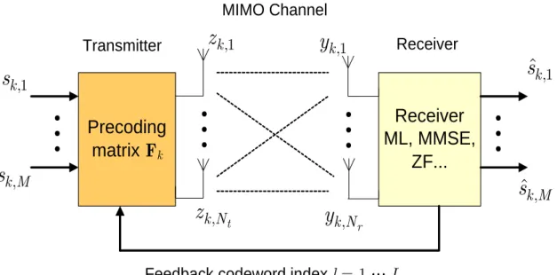
2.1.1 Limited Feedback MIMO Channel Model

The limited feedback MIMO system is illustrated in Figure 2.1. The MIMO system has N transmit antennas and _t N receive antennas. The receiver selects the _r optimal precoder based on current CSI and feeds back the index of the optimal precoder to the transmitter. M different substreams are precoded with the optimal precoder F . Each of the M substreams is modulated independently using the same _k constellation W . This yields a data symbol vector at time slot k of

,1, ,2,..., ,

T k = ⎢⎡_⎣sk sk sk M⎤⎥_⎦

s . s_{k j}_, is the data symbol of the j th substream at time slot k and E_s_k _⎢⎡_⎣s s_{k k}H_⎦_⎥⎤ =E_s⋅I_M . We assume that E_s_k _⎢_⎣⎡s s_{k k}H⎤ =_⎥_⎦ E_s⋅I_M = I_M for convenience.

(20)

Precoding

matrix F

k

#

,1 k

s

Transmitter

Receiver

ML, MMSE,

ZF...

,1

ˆ

_k

s

MIMO Channel Receiver

#

, k M

s

,1 k

z

, _t k N

z

#

, _r k N

y

,1 k

y

,

ˆ

_{k M}

s

#

Feedback codeword index l = 1,…,L

Figure 2.1: Limited feedback MIMO system architecture

The data symbol vector s is multiplied by an _k N_t×M precoder F which is _k selected as a function of the current CSI by using the precoder selection criteria. The transmit signal vector z_k = ⎢_⎣⎡z_k_,1,...,z_{k N}_, _t⎤_⎥_⎦T at time slot k can be written as

, s k = E_M k k

z F s (2.1)

where E is the symbol energy. Assuming perfect timing, synchronization, and _s sampling, the discrete-time equivalent received signal vector can be written as

, s

k = E_M k k k + k

y H F s n (2.2)

where H is the _k N_r×N_t channel matrix and n is the _k N × noise vector at _r 1 time slot k . The entries of H are independent and identically distributed (i.i.d.) _k according to CN(0,1) and the entries of n are independent and distributed _k according to CN

(

0,σ_n2

)

. The received signal vector is decoded by a vector decoder with perfect knowledge of H F that produces a hard decoded symbol vector ˆ_{k k} s . _k

(21)

{

1, ,...,2 N

}

= F F F

F and feeds back the index of the selected precoder to the transmitter over a limited bandwidth, zero-delay feedback link. Each F_k ∈F is assumed to have orthogonal unit column vectors since it follows the form of the optimal, full channel knowledge precoders derived in [9] assuming a maximum singular value constraint of F . The proposed codebook satisfies _k F ⊂ U

(

N M_t,

)

.

We assume that b bits of feedback are available. Thus, the codebook consists of 2b

N = matrices in U

(

N M_t,

)

. In this constraint, codebook design can be converted to a problem of Grassmannian line packing [24]. The limitation of the codebook to 2b matrices allows the designer to constrain the precoding overhead and take full advantage of the limited feedback channel.

2.1.2 Decoding Scheme of Limited Feedback MIMO

Systems

Linear receivers apply an M×N_r matrix G to produce the hard decoded symbol vector ˆs , where ˆ_k s_k =Gy . Criteria will be presented for two different forms _k of G : zero-forcing (ZF) and minimum mean-square error (MMSE).

Zero-Forcing (ZF) Receiver

For a zero-forcing linear receiver, the decoding matrix G is defined as

(

_{k k}

)

+,

=

G H F (2.3)

where ()⋅ is the matrix pseudo-inverse, + H is the channel matrix, and _k F is the _k precoding matrix. Perfect CSI known at the receiver is assumed. The hard decoded symbol vector ˆs from the ZF decoder can be written as _k

(22)

(

)

(

)

( )

(

)

noise signal ˆ . s k k k k k k k k k k s M k k k k E M E M + + + = = + = + s Gy H F H F s H F n I s H F n (2.4)

Minimum Mean-Square Error (MMSE) Receiver

For an MMSE linear receiver, the decoding matrix G is defined as

1 0 _, H H H H k k k k M k k s MN E − ⎛ _⎞⎟ ⎜ _⎟ =⎜_⎜ + _⎟_⎟ ⎜⎝ ⎠ G F H H F I F H (2.5)

where M is the number of substreams, N is the noise power spectrum density, and ₀ s

E is the symbol energy. The hard decoded symbol vector ˆs of the MMSE decoder _k can be written as

( )

signal 1 0 1 0 1 0 ˆ = k k H H H H s k k k k M k k k k k s H H H H k k k k M k k k s H H s k k k k M M k s E MN M E MN E E MN M E − − − = ⎛ _⎞⎟ ⎜ _⎟ = ⎜_⎜ + _⎟_⎟ ⎜⎝ ⎠ ⎛ _⎞⎟ ⎜ _⎟ +⎜_⎜ + _⎟_⎟ ⎜⎝ ⎠ ⎛ _⎞⎟ ⎜ ₊ _⎟ ⎜ _⎟ ⎜ ⎟ ⎜⎝ ⎠ s Gy F H H F I F H H F s F H H F I F H n F H H F I I s noise 1 0 _. H H H H k k k k M k k k s MN E − ⎛ _⎞⎟ ⎜ _⎟ +⎜_⎜ + _⎟_⎟ ⎜⎝F H H F I ⎠ F H n (2.6)

The MMSE receiver is more complex than the ZF receiver. However, it has better performance in noise reduction and reliability.

(23)

2.2 Precoder Selection Criteria

In this section, we will introduce the precoder selection criteria proposed in [16] used for selecting the optimal percoder from a given codebook. Three precoder selection criteria will be introduced here: (1) capacity selection criterion (Capacity-SC), (2) MSE selection criterion (MSE-SC), and (3) minimum singular value selection criterion (MSV-SC).

2.2.1 Capacity Selection Criterion

When the transmitter is precoded with the precoder F , the equivalent channel is HF . The mutual information assuming an uncorrelated complex Gaussian source given H and a fixed F is ( ) ₂ 0 log det _M Es H H . I MN ⎛ _⎞⎟ ⎜ _⎟ = ⎜_⎜ + _⎟_⎟ ⎜⎝ ⎠ F I F H HF (2.7)

The capacity selection criterion is stated as follows:

Capacity Selection Criterion (Capacity-SC):

Pick F such that

( )

arg max , i i I ∈ = F F F F (2.8)

where F is the precoder set. Capacity selection criterion can improve the effective channel capacity and the optimal unquantized precoder is F_opt = V_R, which is proved in [16]. V is the matrix formed from the first M columns of _R V_R and V_R is the right singular matrix of the channel matrix H .

(24)

2.2.2 Mean Square Error Selection Criterion

For a linear MMSE receiver, the precoder is selected to either minimize the trace of the mean square error matrix or minimize the determinant of the mean square error matrix. The linear MMSE decoder is defined as

1 0 _. H H H H M s MN E − ⎛ _⎞⎟ ⎜ _⎟ =⎜_⎜ + _⎟_⎟ ⎜⎝ ⎠ G F H HF I F H (2.9)

The MSE can be expressed as

( ) 1 0 MSE s s H H . M E E M MN − ⎛ _⎞⎟ ⎜ _⎟ = ⎜_⎜ + _⎟_⎟ ⎜⎝ ⎠ F I F H HF (2.10)

Using (2.10), the MSE selection criterion is stated as follows:

Mean Square Error Selection Criterion (MSE-SC):

( )

(

)

arg min MSE ,

i i m ∈ = F F F F (2.11)

where m ⋅ denotes either det()() ⋅ or trace()⋅ . MSE selection criterion can improve the overall system performance and the optimal unquantized precoder is F_opt = V_R which is also proved in [16].

2.2.3 Minimum Singular Value Selection Criterion

For a linear ZF receiver, the precoder is selected to minimize the bound on the average probability of a symbol vector error. The linear ZF decoder is defined as

( )+, =

G HF (2.12)

where ()⋅ is the matrix pseudo-inverse. From [17], the SNR of the k th substream is + given by

(25)

(ZF) 1 0 _, SNR_k s , H H k k E MN − = ⎡ ⎤ ⎢ ⎥ ⎣F H HF⎦ (2.13) where A_{k k}−_,1 is entry (k k of , ) A−1.

The work in [17] shows that in order to minimize a bound on the average probability of a symbol vector error, the minimum substream SNR must be maximized. Using a selection criterion based on the minimum SNR requires the computation of the SNR of all substreams. The high computational complexity results in hard implementation. For the reason, [17] shows that the minimum SNR for ZF can be bounded by { } (ZF) (ZF) 2 min min ₁ 0 SNR min SNR_k s , k M E MN λ ≤ ≤ = ≥ HF (2.14)

where λ_min{HF is the minimum singular value of HF . Using (2.14), the minimum } singular value selection criterion is stated as follows:

Minimum Singular Value Selection Criterion (MSV-SC):

{

}

min arg max . i i λ ∈ = F F HF F (2.15)

From [17], the minimum singular value selection criterion provides a close approximation to maximizing the minimum SNR for ZF receiver and the optimal unquantized precoder is F_opt = V_R which is also proved in [16].

(26)

2.3 Codebooks for MIMO Precoding Scheme in

IEEE 802.16-2005

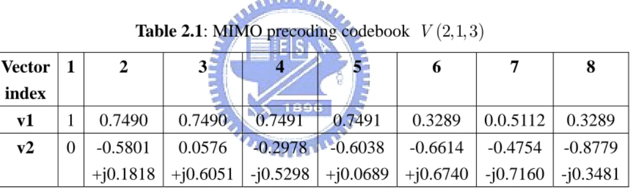
Codebooks with different dimensions and sizes are defined in IEEE 802.16-2005 standard [25]. All codebooks are divided into two kinds: 3-bit codebooks and 6-bit codebooks. The codebooks for 2x1, 3x1, and 4x1 with 3-bit feedback index are listed in Table 2.1, Table 2.2, and Table 2.3. The notation V N S L

(

_t, ,

)

denotes the vector codebook, which consists of 2L complex, unit vectors of a dimension N . S _t denotes the number of substreams. The interger L is the number of bits required for the index that can indicate any matrix in the codebook.

Table 2.1: MIMO precoding codebook V(2,1, 3) Vector index 1 2 3 4 5 6 7 8 v1 1 0.7490 0.7490 0.7491 0.7491 0.3289 0.0.5112 0.3289 v2 0 -0.5801 +j0.1818 0.0576 +j0.6051 -0.2978 -j0.5298 -0.6038 +j0.0689 -0.6614 +j0.6740 -0.4754 -j0.7160 -0.8779 -j0.3481

Table 2.2: MIMO precoding codebook V(3,1, 3) Vector index 1 2 3 4 5 6 7 8 v1 1 0.5 0.5 0.5 0.5 0.4954 0.5 0.5 v2 0 -0.7201 -0.3126i -0.0659 +0.1371i -0.0063 +0.6527i 0.7171 +0.3202i 0.4819 -0.4517i 0.0686 -0.1386i -0.0054 -0.654i v3 ₀ 0.2483 -0.2684i -0.6283 -0.5763i 0.4621 -0.3321i -0.2533 +0.2626i 0.2963 -0.4801i 0.6200 +0.5845i -0.4566 +0.3374i

(27)

Table 2.3: MIMO precoding codebook V(4,1, 3) Vector index 1 2 3 4 5 6 7 8 v1 1 0.3780 0.3780 0.3780 0.3780 0.3780 0.3780 0.3780 v2 0 -0.2698 -0.5668i -0.7103 +0.1326i 0.2830 -0.094i -0.0841 +0.6478i 0.5247 +0.3532i 0.2058 -0.1369i 0.0618 -0.3332i v3 0 0.5957 +0.1578i -0.235 -0.1467i 0.0702 -0.8261i 0.0184 +0.049i 0.4115 +0.1825i -0.5211 +0.0833i -0.3456 +0.5029i v3 0 0.1587 -0.2411i 0.1371 +0.4893i -0.2801 +0.0491i -0.3272 -0.5662i 0.2639 +0.4299i 0.6136 -0.3755i -0.5704 +0.2133i

In IEEE 802.16-2005 standard [25], three operations are employed and they employ floating point arithmetric in IEEE Standard 754, whose final results are rounded to four decimal places. The first operation is introduced as follows and generates an unitary N×N matrix H v using an ( ) N × vector v as 1

( ) 1 , , , otherwise H H I p ⎧ = ⎪⎪⎪ = ⎨ ⎪ − ⎪⎪⎩ I v e v ww (2.16) where w= −v e , ₁ e₁ =[1, 0,..., 0]T, 2 ₂ H p =

w w , and I is the identity matrix. The second operation generates an N×(M + unitary matrix from a unit 1) N × 1 vector and a unitary (N − ×1) M matrix as

( )

(

)

(

)

( ) 1 1 1 0 0 0 , , 0 N N M N N M HC _{− ×} H − × ⎡ ⎤ ⎢ ⎥ ⎢ ⎥ ⎢ ⎥ = ⎢ ⎥ ⎢ ⎥ ⎢ ⎥ ⎢ ⎥ ⎢ ⎥ ⎣ ⎦ v A v A (2.17)

where N − ≥1 M and the (N − ×1) M unitary matrix has property A AH =I . The third operation generates an N×M matrix from a unit N × vector, 1 v , by _N taking the last N − columns of 1 H v

(

_N

)

as

(28)

(

_N

)

(

_N

)

_:,2:_N.

HE v =H v (2.18)

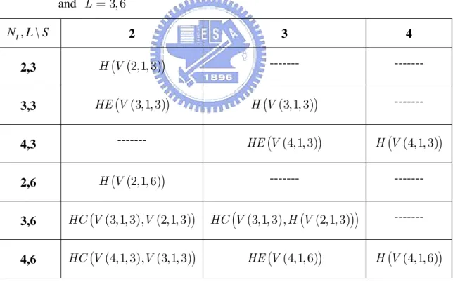
The three operations jointly generate eleven matrix codebooks from vector codebooks as listed in Table 2.4. Table 2.4 contains the operations to generate codebooks V N S L

(

_t, ,

)

for N =_t 2, 3, 4, S =2, 3, 4, and L =3,6. The set notation

(

_t,1,

)

V N L in the input arguments of the operations denotes that each vector in the codebook V N

(

_t,1,L

)

is sequentially taken as an input to the operations. The output of the operation with one or more codebooks as input arguments is also a codebook.

Table 2.4: Operations to generate codebooks V N S L

(

_t, ,

)

for N =_t 2, 3, 4, S =2, 3, 4, and L =3, 6 , \ t N L S 2 3 4 2,3 H V

(

(2,1, 3)

)

--- --- 3,3 HE V

(

(3,1, 3)

)

H V

(

(3,1, 3)

)

--- 4,3 --- HE V

(

(4,1, 3)

)

H V

(

(4,1, 3)

)

2,6 H V

(

(2,1, 6)

)

--- --- 3,6 HC V

(

(3,1, 3 ,)V(2,1, 3)

)

HC V

(

(3,1, 3 ,) H V

(

(2,1, 3)

)

--- 4,6 HC V

(

(4,1, 3 ,)V(3,1, 3)

)

HE V

(

(4,1, 6)

)

H V

(

(4,1, 6)

)

(29)

2.4 Summary

In this chapter, the limited feedback MIMO system is introduced. The receiver feeds back the index of the optimal precoder which is selected by the proposed precoder selection criteria to the transmitter. The transmitter does not need to know the current CSI. For linear receivers, three precoder selection criteria, Capacity-SC, MSE-SC, and MSV-SC are proposed to select the optimal precoder based on current CSI. Different precoder selection criteria can be chosen according to the system requirements. IEEE 802.16-2005 standard supports the limited feedback MIMO precoding scheme and the codebooks with different dimensions and sizes are also defined in this standard.

(30)

Equation Section (Next)

Chapter 3 Single-Mode Limited Feedback

Precoding for MISO Systems

Limited feedback precoding for MIMO system is a popular technique used to improve system reliability for wireless communications. The single-mode limited feedback system is a system that has only one codebook. In general, the average feedback rate of the limited feedback system is fixed in a transmission. Under this condition, the performance of the single-mode limited feedback system is affected by the codebook size and the variation of the channel.

In the practical communication system, the transmitter has multiple antennas and the receiver generally has only one antenna. Obviously, it is a MISO communication system. The transmit beamforming is a powerful technique for enhancing the MISO system performance. With perfect CSI, the transmit beamforming can achieve optimal performance in the MISO system in terms of maximizing the received SNR [11]-[13].

In Chapter 3, single-mode limited feedback systems are presented first. We consider the transmit beamforming scheme and MISO channel model in this thesis. The channel characteristics are modeled by the first-order Markov channel model. Then the transmit beamforming codebooks in IEEE 802.16-2005 standard are given and used in the computer simulation. Finally, the simulation results are illustrated and discussed.

(31)

3.1 Single-Mode Limited Feedback Systems

The single-mode limited feedback system is a system that has only one codebook, either large-size or small-size. Under a fixed average feedback rate, the system with a small-size codebook feeds back less bits more often and that with a large-size codebook feeds back more bits less often. For example, if the average feedback rate is fixed at three bits per frame, the receiver with a 3-bit codebook feeds back three bits per frame and that with a 6-bit codebook feeds back six bits per two frames. Figure 3.1 illustrates the single-mode limited feedback system architecture in the MIMO channel.

Figure 3.1: Single-mode limited feedback system architecture

Because the receiver generally has only one receive antenna in the practical communication system, we consider the MISO channel model and the transmit beamforming scheme in this thesis. In this section, we will introduce the first-order Markov MISO channel model which is assumed in this thesis. The decoding scheme of the single-mode limited feedback MISO system will be given in the following.

(32)

3.1.1 First-Order Markov MISO Channel Model

Consider a MISO channel model with N transmit antennas and single receive _t antenna. In the frame-based transmission, let h denotes the channel coefficient k_j between the j th transmit antenna and the receive antenna. k is the frame index. We collect h ’s into the channel vector k_j ₁, ,...,₂

t

k k k k = ⎢⎡_⎣h h hN ⎤⎥_⎦

h . f is the beamformer and _k k

g is the gain control factor for the k th frame. s is the 1 L_k × data symbol vector and ˆs is the 1 L_k × detected symbol vector for the k th frame, where L is the frame length. We assume that

k H k k L ⎡ _{⎤ =} ⎢ ⎥ ⎣ ⎦ s

E s s I for power constraint reasons. The

transmit beamforming for MISO system is illustrated in Figure 3.2.

Figure 3.2: Transmit beamforming scheme for MISO system

The data symbol vector s is multiplied by an _k N × beamformer _t 1 f which _k is selected as a function of the current CSI by using the proposed beamformer selection criterion. Assuming perfect timing, synchronization, and sampling, the discrete-time

(33)

equivalent received signal can be written as

, k = k k k + k

y h f s n (3.1)

where h is the 1_k ×N_t channel vector and n is the 1 L_k × noise vector for the

k th frame. The entries of n are independent and distributed according to _k

(

_0, 2

)

n

σ

CN . We assume that the channel is quasi-static in a frame period and all elements of h are independent identically distributed (i.i.d.) according to a complex _k Gaussian distribution with zero-mean and unit variance; that is

(

,

)

.

t

k N

h ∼ CN 0 I (3.2)

The time-varying property of the MISO channel can be characterized by the first-order Markov channel model. The first-order Markov channel model is only characterized by the one-tap temporal-correlation coefficient ρ . The channel vector for the (k +1)th frame is given by

1 ,

k+ = ρ k + Δ

h h h (3.3)

where k is the frame index,

(

, 1( )

)

t

N

ρ

Δh∼ CN 0 − I , and ρ is the temporal-correlation coefficient ( 0≤ ≤ ). A small ρ 1 ρ(=0) implies the fast fading environment and a large (ρ =1) corresponds to the time-invariant channel. The feature of the first-order Markov channel model is that the channel can be characterized by only one-tap temporal-correlation coefficient. The channel can be modeled as a time-invariant channel with a large ρ or a time-varying channel with a small ρ . This channel model is also widely used in other research papers [13],[28]-[31].

(34)

3.1.2 Decoding Scheme of Limited Feedback MISO

Systems

In MISO systems, linear receivers apply a gain control factor g to produce the _k hard decoded symbol vector ˆs , where ˆ_k s_k =g_{k k}y . For a zero-forcing linear receiver, the gain control factor g is defined as _k

(

)

,

k k k

g = h f + (3.4)

where ()⋅ is the matrix pseudo-inverse, + h is the 1_k ×N_t channel vector, and f is _k the N × transmit beamformer. The hard decoded symbol vector ˆ_t 1 s from the ZF _k decoder can be written as

(

)

(

)

(

)

signal noise

ˆ_k =g_{k k} = _{k k} + _{k k k} + _{k k} + _k = _k + _{k k} + _k.

s y h f h f s h f n s h f n (3.5)

The decoded symbol vector ˆs will be fed into the demodulator and the decoded _k binary data stream will be produced from the demodulator.

When the transmitter is precoded with the beamformer f , the equivalent channel _k is h f . _{k k} h is the 1_k ×N_t channel vector and f is the _k N × beamformer. _t 1 Actually, h f is a received power gain provided by the channel and the beamformer. _{k k} The larger the received power gain is, the better the system performance is. The beamformer selection criterion is stated as follows:

Maximum Signal-to-Noise Ratio Selection Criterion (MSNR-SC):

Pick f such that _k

2 arg max , i k = _∈ k i f f h f F (3.6)

where F is the beamformer set and | |⋅ is the square of the vector norm. The 2 transmit beamforming scheme can increase the received power gain and improve the system performance.

(35)

3.2 Transmit Beamforming Codebooks in IEEE

802.16-2005

IEEE 802.16-2005 standard [25] supports the limited feedback MIMO precoding scheme. The transmit beamforming is a special case of the MIMO precoding with

1

M = and N_r = , where M is the number of substreams and 1 N is the number _r

of receive antennas. In this standard, all codebooks are divided into two kinds: 3-bit codebooks and 6-bit codebooks. The transmit beamforming (M = ) codebooks are 1 listed in Table 3.1. The notation V N S L

(

_t, ,

)

denotes the vector codebook, which consists of 2L complex, unit vectors of a dimension N . S denotes the number of _t substreams. All the codewords of V(2,1, 3), V(3,1, 3), and V(4,1, 3) are listed in Table 2.1, Table 2.2, and Table 2.3.

Table 3.1: Transmit beamforming codebooks in IEEE 802.16-2005 standard , \ t N S L 3 6 2,1 V(2,1, 3) V(2,1, 6) 3,1 V(3,1, 3) V(3,1, 6) 4,1 V(4,1, 3) V(4,1, 6)

In IEEE 802.16-2005 standard [25], two vector codebooks V(3,1, 6) and (4,1, 6)

V are generated as follows. All the vector codewords v , _i i =2,...,2L are derived from the first codeword v as ₁

1 ( ) ( )i H( ) , for 2,..,2 ,L i =H Q H i− i= v s u s v (3.7) 1_{, for} _{2,..,2 ,} j L i = ie−φ i= v v (3.8)

(36)

where 1 2 2 2 2 ( ) diag j L u i,..., j L uNt i i Q e e π π ⋅ ⋅ ⋅ ⋅ ⋅ ⋅ ⎛ _⎞⎟ ⎜ _⎟ ⎜ = _⎜_⎜ ⎟_⎟ ⎟⎟ ⎜⎝ ⎠ u is a diagonal matrix, ₁,..., t N u u ⎡ ⎤ = ⎢_⎣ ⎥_⎦ u is an interger vecror, ( ) 2 2 1 1 1 1, ,..., t t t T j j N N N t e e N π π ⋅ ⋅ − ⎡ ⎤ ⎢ ⎥ = ⎢ ⎥ ⎢ ⎥ ⎢ ⎥ ⎣ ⎦

v , and φ is the phase of the _i

first entry of v . _i H ⋅ is defined in the Equation (2.16). The parameters for the ( ) generation of V(3,1, 6) and V(4,1, 6) are listed in Table 3.2 and the codewords of

(3,1, 6)

V is listed in Table 3.3.

Table 3.2: Generating parameters for V(3,1, 6) and V(4,1, 6) t N L u in Qi( )u s in H( )s 3 6 [1,26, 57 ] [1.2518−j0.6409, 0.4570− −j0.4974, 0.1177+ j0.2360]T 4 6 [1, 45,22, 49 ] [ ] 1.3954 0.0738, 0.0206 0.4326, 0.1658 0.5445, 0.5487 0.1599T j j j j − + − − −

We can follow the above algorithms to generate the vector codebooks V(3,1, 6) and V(4,1, 6). Unfortunately, IEEE 802.16-2005 standard does not provide the generating parameters for the codebook V(2,1, 6).

The 6-bit codebook provides sixty-four beamformers to be selected. It has higher probability that the optimal beamformer which is closest to the unquantized optimal beamformer can be selected. But the receiver needs to feed back six bits in a transmission. Although the 3-bit codebook provides only eight beamformers to be selected, the receiver needs to feed back only three bits in a transmission.

(37)

Table 3.3: MIMO precoding codebook V(3,1, 6) Matrix index (binary) Column 1 Matrix index (binary) Column 1 0.5774 0.5437 –0.2887 + j0.5000 –0.1363 – j0.4648 000000 –0.2887 – j0.5000 100000 0.4162 + j0.5446 0.5466 0.5579 0.2895 – j0.5522 –0.6391 +j0.3224 000001 0.2440 + j0.5030 100001 –0.2285 – j0.3523 0.5246 0.5649 –0.7973 – j0.0214 0.6592 – j0.3268 000010 –0.2517 – j0.1590 100010 0.1231 + j0.3526 0.5973 0.484 0.7734 + j0.0785 –0.6914 – j0.3911 000011 0.1208 + j0.1559 100011 –0.3669 +j0.0096 0.4462 0.6348 –0.3483 – j0.6123 0.5910 + j0.4415 000100 –0.5457 + j0.0829 100100 0.2296 – j0.0034 0.6662 0.4209 0.2182 + j0.5942 0.0760 – j0.5484 000101 0.3876 – j0.0721 100101 –0.7180 +j0.0283 0.412 0.6833 0.3538 – j0.2134 –0.1769 +j0.4784 000110 –0.8046 – j0.1101 100110 0.5208 – j0.0412 0.684 0.4149 –0.4292 + j0.1401 0.3501 + j0.2162 000111 0.5698 + j0.0605 100111 –0.7772 – j0.2335 0.4201 0.6726 0.1033 + j0.5446 –0.4225 – j0.2866 001000 –0.6685 – j0.2632 101000 0.5061 + j0.1754 0.6591 0.419 –0.1405 – j0.6096 –0.2524 + j0.6679 001001 0.3470 + j0.2319 101001 –0.5320 – j0.1779 0.407 0.6547 –0.5776 + j0.5744 0.2890 – j0.6562 001010 –0.4133 + j0.0006 101010 0.1615 + j0.1765

(38)

Table 3.3: MIMO precoding codebook V(3,1, 6) (continued) Matrix index (binary) Column 1 Matrix index (binary) Column 1 0.6659 0.3843 0.6320 – j0.3939 –0.7637 + j0.3120 001011 0.0417 + j0.0157 101011 –0.3465 + j0.2272 0.355 0.69 –0.7412 – j0.029 0.6998 + j0.0252 001100 –0.3542 + j0.445 101100 0.0406 – j0.1786 0.7173 0.3263 0.4710 + j0.3756 –0.4920 – j0.3199 001101 0.1394 – j0.3211 101101 –0.4413 + j0.5954 0.307 0.7365 –0.0852 – j0.414 0.0693 + j0.4971 001110 –0.5749 + j0.629 101110 0.2728 – j0.3623 0.74 0.3038 –0.3257 + j0.346 0.3052 – j0.2326 001111 0.3689 – j0.3007 101111 –0.6770 + j0.5496 0.3169 0.727 0.4970 + j0.1434 –0.5479 – j0.0130 010000 –0.6723 + j0.424 110000 0.3750 – j0.1748 0.7031 0.3401 –0.4939 – j0.429 0.4380 + j0.5298 010001 0.2729 – j0.0509 110001 –0.5470 + j0.3356 0.3649 0.6791 0.1983 + j0.7795 –0.1741 – j0.7073 010010 –0.3404 + j0.3224 110010 0.0909 – j0.0028 0.6658 0.3844 0.2561 – j0.6902 –0.1123 + j0.8251 010011 –0.0958 – j0.0746 110011 –0.1082 + j0.3836 0.3942 0.6683 –0.3862 + j0.6614 0.5567 – j0.3796 010100 0.0940 + j0.4992 110100 –0.2017 – j0.2423 0.6825 0.394 0.5632 + j0.0490 –0.5255 + j0.3339 010101 –0.1901 – j0.4225 110101 0.2176 + j0.6401

(39)

Table 3.3: MIMO precoding codebook V(3,1, 6) (continued) Matrix index (binary) Column 1 Matrix index (binary) Column 1 0.3873 0.6976 –0.4531 – j0.0567 0.2872 + j0.3740 010110 0.2298 + j0.7672 110110 –0.0927 – j0.5314 0.7029 0.3819 –0.1291 + j0.4563 –0.1507 – j0.3542 010111 0.0228 – j0.5296 110111 0.1342 + j0.8294 0.387 0.6922 0.2812 – j0.3980 –0.5051 + j0.2745 011000 –0.0077 + j0.7828 111000 0.0904 – j0.4269 0.6658 0.4083 –0.6858 – j0.0919 0.6327 – j0.1488 011001 0.0666 – j0.2711 111001 –0.0942 + j0.6341 0.4436 0.6306 0.7305 + j0.2507 –0.5866 – j0.4869 011010 –0.0580 + j0.4511 111010 –0.0583 – j0.1337 0.5972 0.4841 –0.2385 – j0.7188 0.5572 + j0.5926 011011 –0.2493 – j0.0873 111011 0.0898 + j0.3096 0.5198 0.5761 0.2157 + j0.7332 0.1868 – j0.6492 011100 0.2877 + j0.2509 111100 –0.4292 – j0.1659 0.571 0.5431 0.4513 – j0.3043 –0.1479 + j0.6238 011101 –0.5190 – j0.3292 111101 0.4646 + j0.2796 0.5517 0.5764 –0.3892 + j0.3011 0.4156 + j0.1263 011110 0.5611 + j0.3724 111110 –0.4947 – j0.4840 0.5818 0.549 0.1190 + j0.4328 –0.3963 – j0.1208 011111 –0.3964 – j0.5504 111111 0.5426 + j0.4822

(40)

3.3 Computer Simulations

In IEEE 802.16-2005 standard [25], all codebooks can be divided into two kinds: 3-bit codebooks and 6-bit codebooks. Under a fixed average feedback rate, two modes are defined as follows: (1) Mode I is defined in which the transmitter is precoded with the 6-bit beamformer and the receiver feeds back six bits per two frames; (2) Mode II is defined in which the transmitter is precoded with the 3-bit beamformer and the receiver feeds back three bits per frame. The schemes of Mode I and Mode II are illustrated in Figure 3.3.

Figure 3.3: Transmit beamforming schemes of Mode I and Mode II

In the following, we illustrate the performances of the single-mode limited feedback MISO system. Besides, we also consider a MISO-OFDM system in the simulations and illustrate the performances of the single-mode limited feedback MISO-OFDM system. Under a fixed average feedback rate at three bits per frame or per OFDM symbol period, the schemes of Mode I and Mode II for single-carrier systems and multi-carrier systems are commented in Table 3.4.

(41)

Table 3.4: Schemes of Mode I and Mode II for single-carrier and multi-carrier systems Fixed average feedback rate at 3 bits/frame (or OFDM symbol period)

Single-Carrier (MISO) Multi-Carrier (MISO-OFDM) Mode I feed back 6 bits per two frames feed back 6 bits per tone and per two

OFDM symbol periods

Mode II feed back 3 bits per frame feed back 3 bits per tone and per OFDM symbol period

(a) Single-mode limited feedback MISO system

Table 3.5 lists all parameters used in this simulation. This simulation uses 16-QAM modulation and one data substream on a 4× wireless system. The transmit 1 beamforming codebooks in IEEE 802.16-2005 are applied in the simulation. The average feedback rate is fixed at three bits per frame. In Mode I, the receiver feeds back six bits to the transmitter per two frames; in Mode II, the receiver feeds back three bits to the transmitter per frame. Each frame consists of 128 symbols and each transmission consists of 16 frames.

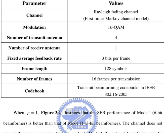
The channel is assumed to be quasi-static and Rayleigh fading. The channel gains of two consecutive frames follow the first-order Markov channel model (Equation (3.3)). The elements of the random perturbation Δh in Equation (3.3) are assumed to be independent identically distributed (i.i.d.) complex Gaussian random variables with zero-mean and variance (1−ρ). SNR is defined as the ratio of the average received signal power to the average received noise power. Perfect channel knowledge known at the receiver and the error-free feedback channel are also assumed in the simulation. SER performances of the single-mode limited feedback MISO system (operating in Mode I or Mode II) with ρ =1, 0.9, 0.8, 0.7 are shown in Figures 3.4-3.7.

(42)

Table 3.5: Simulation environment of the single-mode limited feedback MISO system

Parameter Values

Channel Rayleigh fading channel

(First-order Markov channel model)

Modulation 16-QAM

Number of transmit antenna 4

Number of receive antenna 1

Fixed average feedback rate 3 bits per frame

Frame length 128 symbols

Number of frames 16 frames per transmission

Codebook Transmit beamforming codebooks in IEEE 802.16-2005

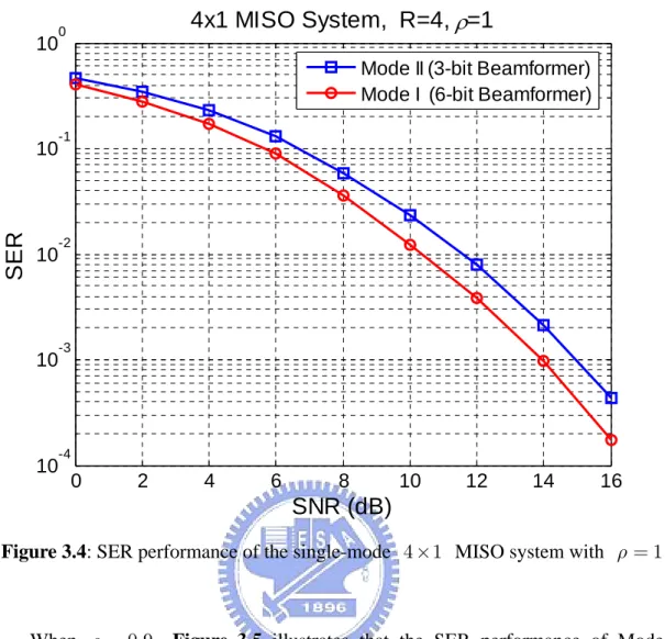
When ρ = , Figure 3.4 illustrates that the SER performance of Mode I (6-bit 1 beamformer) is better than that of Mode II (3-bit beamformer). The channel does not vary in the two consecutive frame periods. In Mode I, the optimal beamformer can be selected from the 6-bit codebook (sixty-four beamformers) at the start of the first frame of the two consecutive frames, and it is also optimal for the channel of the second frame. In Mode II, the optimal beamformer is selected from the 3-bit codebook (eight beamformers) at the start of the first frame, and it can be reselected at the start of the second frame. Because the optimal beamformer selected from the 6-bit codebook is closer to the unquantized optimal beamformer than that selected from the 3-bit codebook, the SER performance of Mode I is better than that of Mode II.

(43)

0 2 4 6 8 10 12 14 16 10-4 10-3 10-2 10-1 100

SNR (dB)

SER

4x1 MISO System, R=4, ρ=1

Mode II (3-bit Beamformer) Mode I (6-bit Beamformer)

Figure 3.4: SER performance of the single-mode 4× MISO system with 1 ρ = 1

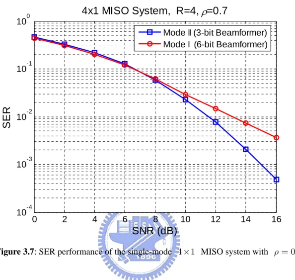
When ρ =0.9, Figure 3.5 illustrates that the SER performance of Mode I becomes slightly poorer than that in Figure 3.4. The curve of Mode I crosses the curve of Mode II at SNR=14 dB. When ρ =0.8 , Figure 3.6 shows that the SER performance of Mode I becomes poorer than that in Figure 3.5. The curve of Mode I crosses the curve of Mode II at SNR=10 dB. When ρ =0.7, Figure 3.7 shows that the SER performance of Mode II is better than that of Mode I.

The reason that the SER performance of Mode I becomes poorer as ρ decreases is that the beamformer which is optimal for the channel of the k th frame is not always optimal for that of the (k +1)th frame. The nonoptimal beamformer decreases the average received power gain over the (k +1)th frame. The single-mode system operating in Mode I loses diversity gain as ρ decreases.

(44)

0 2 4 6 8 10 12 14 16 10-4 10-3 10-2 10-1 100

SNR (dB)

SER

4x1 MISO System, R=4, ρ=0.9

Figure 3.5: SER performance of the single-mode 4× MISO system with 1 ρ =0.9

0 2 4 6 8 10 12 14 16 10-4 10-3 10-2 10-1 100

SNR (dB)

SER

4x1 MISO System, R=4, ρ=0.8

(45)

0 2 4 6 8 10 12 14 16 10-4 10-3 10-2 10-1 100

SNR (dB)

SER

4x1 MISO System, R=4, ρ=0.7

Figure 3.7: SER performance of the single-mode 4× MISO system with 1 ρ =0.7

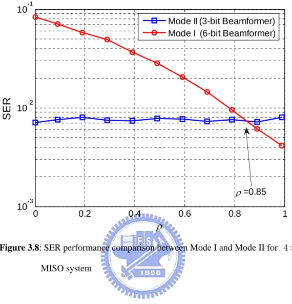
Figure 3.8 shows the SER performance comparison between Mode I and Mode II under a fixed SNR=12 dB. The two lines cross at about ρ = 0.85. Figure 3.8 shows that when the channel is subject to high temporal correlation (ρ ≥0.85), Mode I outperforms Mode II whereas with ρ <0.85 the latter yields better performance. It is obviously observed that Mode I is suitable to be used in the high temporal-correlation channel and Mode II is suitable to be used in the low temporal-correlation channel. From the simulation results, we observed that the single-mode limited feedback system (either Mode I or Mode II) is not robust enough in mobile environments.

(46)

0 0.2 0.4 0.6 0.8 1 10-3 10-2 10-1

ρ

SER

ρ =0.85

Figure 3.8: SER performance comparison between Mode I and Mode II for 4× 1 MISO system

(47)

(b) Single-mode limited feedback MISO-OFDM system

We consider a MISO-OFDM system and Table 3.6 lists all parameters used in this simulation. This simulation uses 16-QAM modulation and 128 subcarriers in the MISO-OFDM system. The multipath Rayleigh fading channel is used in the simulation. The channel gains of two consecutive OFDM symbol periods follow the first-order Markov channel model (Equation (3.3)), and the relative delays and the average power follow the parameters of the channel model defined in ITU-R M.1225 [37]. The elements of the random perturbation Δh in Equation (3.3) are assumed to be i.i.d. zero-mean complex Gaussian with variance (1−ρ). SNR is defined as the ratio of the average received signal power to the average received noise power after DFT. Perfect channel knowledge known at the receiver and the error-free feedback channel are also assumed in the simulation.

The parameters of the simulation environment of the MISO-OFDM system follow IEEE 802.16-2005 [25] and are stated as follows: The FFT length is 128. The bandwidth is 2.5MHz and the sampling frequency is 2.8 MHz. The sampling time is 357.14 ns and the subcarrier spacing is 21.875 kHz. The ratio of CP time is 1/4. The OFDM symbol time is 57.143 us. Each frame consists of 16 OFDM symbols.

The transmit beamforming codebooks in IEEE 802.16-2005 are applied in the simulation. The average feedback rate is fixed at three bits per tone and per OFDM symbol period. In Mode I, the receiver feeds back six bits to the transmitter per tone and per two OFDM symbol periods; in Mode II, the receiver feeds back three bits to the transmitter per tone and per OFDM symbol period. The transmit symbols are precoded with the beamformers tone by tone and we assume that all subcarriers are independent. SER performances of the single-mode limited feedback MISO-OFDM systems with ρ =1, 0.9, 0.8, 0.7 are shown in Figures 3.9-3.12.

(48)

Table 3.6: Simulation environment of the single-mode limited feedback MISO-OFDM system

Parameter Values

Channel Multipath Rayleigh fading channel (First-order Markov channel model)

Tap (ITU-R M.1225) 1 2 3 4 5 6 Relative delay (ns) 0 310 710 1090 1730 2510 Average power (dB) 0 -1 -9 -10 -15 -20 Bandwidth 2.5 MHz FFT length 128 Sampling frequency 2.8 MHz Subcarrier spacing 21.875 kHz

Useful symbol time 45.714 us

Ratio of CP time 1/4

CP time 11.429 us

Symbol time 57.143 us

Sampling time 357.14 ns

Frame length 16 OFDM symbols

Modulation 16-QAM

Number of transmit antenna 4

Number of receive antenna 1

Fixed average feedback rate 3 bits per OFDM symbol period Codebook Transmit beamforming codebooks in IEEE

(49)

0 2 4 6 8 10 12 14 16 10-4 10-3 10-2 10-1 100

SNR (dB)

SER

4x1 MISO-OFDM System, R=4, ρ=1

Figure 3.9: SER performance of the single-mode 4× MISO-OFDM system 1 with ρ = 1

When ρ = , Figure 3.9 illustrates that the SER performance of Mode I is also 1 better than that of Mode II in the MISO-OFDM system. The channel does not vary in the two consecutive OFDM symbol periods. In Mode I, the optimal beamformers for all subcarriers can be selected from the 6-bit codebook at the start of the first OFDM symbol of the two consecutive OFDM symbols, and they are also optimal for the channels of the second OFDM symbol time. In Mode II, the optimal beamformers are selected from the 3-bit codebook at the start of the first OFDM symbol, and they will be reselected at the start of the second OFDM symbol. Because the optimal beamformers selected from the 6-bit codebook are closer to the unquantized optimal beamformers for all subcarriers than that selected from the 3-bit codebook, the SER performance of Mode I is always better than that of Mode II.

(50)

0 2 4 6 8 10 12 14 16 10-4 10-3 10-2 10-1 100

SNR (dB)

SER

4x1 MISO-OFDM System, R=4, ρ=0.9

Figure 3.10: SER performance of the single-mode 4× MISO-OFDM system 1 with ρ =0.9

When ρ =0.9, Figure 3.10 illustrates that the SER performance of Mode I also becomes slightly poorer than that in Figure 3.9. Two lines cross at SNR=14 dB. When

0.8

ρ = , Figure 3.11 shows that the SER performance of Mode I becomes poorer than that in Figure 3.10. The curve of Mode I crosses the curve of Mode II at SNR=10 dB. When ρ =0.7, Figure 3.12 shows that the SER performance of Mode II is better than that of Mode I.

The reason that the SER performance of Mode I becomes poorer as ρ decreases is that the beamformers which are optimal for the channel of the k th OFDM symbol time are not always optimal for the channel of the (k +1)th OFDM symbol time. The nonoptimal beamformers decrease the average received power gain and diversity gain over the (k +1)th OFDM symbol time as ρ decreases.

(51)

0 2 4 6 8 10 12 14 16 10-4 10-3 10-2 10-1 100 SNR (dB) SER 4x1 MISO-OFDM System, R=4, ρ=0.8

Figure 3.11: SER performance of the single-mode 4× MISO-OFDM system with 1 0.8 ρ = 0 2 4 6 8 10 12 14 16 10-4 10-3 10-2 10-1 100 SNR (dB) SER 4x1 MISO-OFDM System, R=4, ρ=0.7

Figure 3.12: SER performance of the single-mode 4× MISO-OFDM system with 1 0.7

(52)

0 0.2 0.4 0.6 0.8 1 10-3 10-2 10-1

ρ

SER

ρ =0.85

Figure 3.13: SER performance comparison between Mode I and Mode II for 4 1× MISO-OFDM system

Figure 3.13 shows the SER performance comparison between Mode I and Mode II for 4× MISO-OFDM system under a fixed SNR=12 dB. Two lines cross at about 1

0.85

ρ = . Figure 3.13 shows that when the channel is subject to high temporal correlation (ρ ≥0.85), Mode I outperforms Mode II whereas with ρ <0.85 the latter yields better performance.

We compare the above simulation results with that of MISO systems. It is obviously observed that the results of the MISO-OFDM system are similar to that of the MISO system because the multipath channel response can be reduced into a multiplicative constant on a tone-by-tone basis by DFT at the receiver and all subcarriers are independent. The properties of the OFDM system will be given in Chapter 4.

(53)

3.4 Summary

The single-mode limited feedback system has been introduced in this chapter. We consider the transmit beamforming scheme and MISO channel model in this thesis and use the first-order Markov channel to model the temporal-correlation channels. The transmit beamforming codebooks in IEEE 802.16-2005 standard are applied in our simulation. The results show that the performance of Mode I becomes poorer as ρ decreases in the MISO system and in the MISO-OFDM system. Obviously, the single-mode limited feedback system is not robust enough in mobile environments. Mode I is suitable to be used in the high temporal-correlation channel and Mode II is suitable to be used in the low temporal-correlation channel.

於時間相關通道下之雙模式有限回授傳送波束形成技術

國 立 交 通 大 學

電信工程學系碩士班

碩士論文