應用知識擷取與資料倉儲技術分析網路行為

全文

(1)國立交通大學資訊科學系碩士論文. 應用知識擷取與資料倉儲技術分析網路行為 Analyzing Network Behaviors with Knowledge Acquisition and Data Warehousing. 研究生：黃柏智指導教授：曾憲雄. 博士. 中華民國九十四年六月.

(2) 應用知識擷取與資料倉儲技術分析網路行為 Analyzing Network Behaviors with Knowledge Acquisition and Data Warehousing. 研究生：黃柏智. Student：Po-Chih Huang. 指導教授：曾憲雄. Advisor：Shian-Shyong Tseng. 國立交通大學資訊科學系碩士論文. A Thesis Submitted to Institute of Computer and Information Science College of Electrical Engineering and Computer Science National Chiao Tung University in partial Fulfillment of the Requirements for the Degree of Master in Computer and Information Science June 2005 Hsinchu, Taiwan, Republic of China. 中華民國九十四年六月.

(3) 應用知識擷取與資料倉儲技術分析網路行為研究生：黃柏智. 指導教授：曾憲雄博士. 國立交通大學資訊科學系. 摘要. 隨著網路使用量的成長，網路服務的地位變得越來越重要，並且有越來越多的攻擊行為被設計來入侵這些網路服務。許多研究探討了如何有系統化地從各種網路流量之資料來源分析網路入侵行為，但是這些研究所分析的資料來源是平坦的，沒有概念階層輔助的。為了取這些研究方法之所長來監控網路入侵行為，之前的研究中提出了網路入侵偵測系統(NIMS)來整合多種資料來源，並且對這整合的資料進行多維度、多概念層級的網路行為分析。然而這個網路入侵偵測係統的後端分析流程須由管理者手動操作，並且分析的結果跟管理者具有的經驗有高度相關。為了減輕管理者在分析時的負擔，分析網路行為的知識需要先被擷取出來。因此這篇論文中提出了一個行為模組構建之知識擷取(KABMC)程序。行為模組構建之知識擷取程序包含兩個演算法:分別是擷取流程轉換(AFT)演算法以及行為模組擷取(BMA)演算法。擷取流程轉換演算法被用來產生出在知識擷取過程中所用到的基本的知識模組，並且在知識擷取過程中減低專家的負擔。行為模組建構之知識擷取演算法被用來從專家處取得網路行為模組的知識，並且這個演算法可以被實作成一個知識擷取的工具。當網路行為模組的知識被擷取出來之後，該知識會被應用來改進原本的網路入侵偵測系統以減低管理者在分析時的負擔，特別是經驗比較不足的管理者。關鍵字：知識擷取、網路行為、資料倉儲、線上分析處理、資料立方體 I.

(4) Analyzing Network Behavior with Knowledge Acquisition and Data Warehousing Student: Po-Chih Huang. Advisor: Dr. Shian-Shyong Tseng. Depart of Computer and Information Science National Chiao Tung University. Abstract As the growth of network environment dramatically increases, the network-based applications and services become more important, and a variety of network intrusion behaviors have also been developed to intrude these services. There are many researches have developed different systematic approaches to analyze different network traffic sources. But the data sources used in these approaches are flat without concept hierarchy. For monitoring network intrusion by taking advantages of these systematic approaches, A Network Intrusion Monitoring System (NIMS) Architecture is proposed in the previous research to integrate multiple data sources and to analyze network traffic data cross different concept level of each dimension. But the analyzing process of NIMS is manually manipulated by administrators, and the analytical results are highly dependent on the experience of administrators. In order to reduce the effort of administrators during analyzing process, the knowledge of analyzing network behaviors need to be acquired first. Therefore, a Knowledge Acquisition of Behavior Model Construction (KABMC) process is proposed. The KABMC consists of two algorithms: Acquisition Flow Transformation (AFT) Algorithm and Behavior Model Acquisition (BMA) Algorithm. The AFT is used to generate a basic knowledge model for acquiring knowledge and reducing the effort of experts during II.

(5) knowledge acquisition process. The BMA is used to acquire the knowledge of network behaviors from experts, a knowledge acquisition tool could be implemented based on BMA algorithm. After acquiring the knowledge of network behavior models, the knowledge is used to enhance the original NIMS to reduce the analyzing effort of administrator, especially junior administrators.. Keyword: Knowledge Acquisition, Network Behavior, Data warehouse, OLAP, Data Cube.. III.

(6) 誌謝這篇論文的完成，必須感謝許多人的協助與支持。首先必須感謝我的指導教授，曾憲雄老師，由於他耐心的指導和勉勵，讓我得以順利完成此篇論文。此外，在老師的帶領下，這兩年來，除了學習應有的專業知識外，研究上許多觀念的釐清更是讓我受益匪淺，對學術研究的追求有了更深的瞭解。此外，於待人處世的方面也得益不少，而真的十分感激。同時，必須感謝我的口試委員，黃國禎教授、陳年興教授與蔡文能教授，他們對這篇論文提供了不少寶貴的建議。. 其次要感謝三位博士班的學長，林順傑學長、王慶堯學長和曲衍旭學長。除了在網路入侵偵測以及資料倉儲領域上讓我了解不少的知識外，在研究上或是系統的發展上都提供了不少的建議及協助，且這篇論文能夠順利完成也得力於三位學長的幫忙。. 另外也要感謝實驗室的學長、同學以及學弟們，翁瑞鋒學長、宋昱璋、吳政霖、羅仁杰，於論文內容或系統的建置上都給了我協助與建議。同時也感謝我的同學：吳政霖、李育松、陳君翰、宋昱璋、陳瑞言、林易虹以及邱成樑，陪我度過這忙碌以及充實的碩士生涯。最後要感謝我的家人在背後默默支持我完成我的碩士生涯。. 要感謝的人很多，無法一一詳述，在此僅向所有幫助過我的人，致上我最深的謝意。. IV.

(7) Table of Content Abstract (In Chinese)............................................................................................... I Abstract....................................................................................................................II Acknowledgement (In Chinese) ........................................................................... IV Table of Content ......................................................................................................V List of Algorithms ................................................................................................VII List of Tables.........................................................................................................VII List of Figures..................................................................................................... VIII Chapter 1: Introduction ..........................................................................................1 Chapter 2: Related work .........................................................................................4 2.1: DDoS ontology and classification ..................................................................4 2.2: Repertory grid .................................................................................................4 2.3: Traditional analysis approaches for network intrusion...................................8 2.4: Using OLAP for log analysis..........................................................................9 Chapter 3: The Framework of Network Monitoring and Analyzing System... 11 3.1: Knowledge Acquisition for Behavior Model Construction ..........................13 3.1.1: Acquisition Flow Transformation ......................................................13 3.1.2: Behavior Model Acquisition..............................................................14 3.2: Network Monitoring and Analyzing System ................................................14 3.2.1: Data Preprocessing Phase ..................................................................15 3.2.2: Concept Hierarchy and Data Warehouse Construction Phase ...........15 3.2.3: Data Analysis Phase...........................................................................16 Chapter 4: Knowledge Acquisition for Behavior Model Construction.............18 4.1: Acquisition Flow Transformation .................................................................18 4.1.1: Acquisition Flow Transformation Algorithm.....................................20 4.2: Behavior Model Acquisition.........................................................................24 4.2.1: Behavior Model Acquisition Algorithm ............................................27 4.3: Hierarchical relation between behaviors.......................................................34 Chapter 5: Building the Network Monitoring System .......................................36 5.1: Feature Vector Integration ............................................................................36 V.

(8) 5.2: Concept hierarchy and Data warehouse construction...................................38 5.2.1: Concept Hierarchy Construction .......................................................38 5.2.2: Data Warehouse Construction............................................................39 5.2.3: Dimension Table Maintenance ..........................................................41 5.3: Data analysis .................................................................................................41 5.3.1: Behavior model Transformation ........................................................43 5.3.2: Hierarchical relation ..........................................................................46 Chapter 6: Implementation of Analyzing System ...............................................49 Chapter 7: Conclusion and Future Work ............................................................55 Reference ………………………………………………………...……………….57. VI.

(9) List of Algorithms. Algorithm 1: Acquisition Flow Transformation Algorithm………………….20 Algorithm 2: Behavior Model Acquisition Algorithm………………………..27 Algorithm 3: Behavior Model Transformation Algorithm…………………...44. List of Tables Table 4.1 Attribute order after sorting……………………………………………22 Table 4.2 Table of corresponding dependent relation……………………………23 Table 5.1 Fact Table………………………………………………………………..38 Table 5.2 The result of data query………………………………………………...45. VII.

(10) List of Figures Figure 3.1 The System Architecture of Data Analyzing Framework........12 Figure 3.2 Processes of KABMC................................................................13 Figure 4.1 Input and output of AFTA........................................................19 Figure 4.2 Flag attribute and corresponding values .................................21 Figure 4.3 More attribute and corresponding values after step2 ..............21 Figure 4.4 Sub flows of each attribute .......................................................22 Figure 4.5 Generated Acquisition Flow .....................................................24 Figure 4.6 Input and Output of BMAA .....................................................26 Figure 4.7 Smurf and Ping flood…………………………………………30 Figure 4.8 FTP and SMTP .........................................................................31 Figure 4.9 After adding SYN flood and TCP flood....................................32 Figure 4.10 More detail of each behavior..................................................33 Figure 4.11 The Behavior profile of ping flood .........................................33 Figure 4.12 Hierarchical relations between DDoS behaviors...................35 Figure 5.1 Concept levels of each dimension of network traffic data ......39 Figure 5.2 Cube schema for constructing data warehouse.......................40 Figure 5.3 Comparison between original and enhanced workflow ..........42 Figure 5.4 General process step of CMCA ................................................43 Figure 5.5 original data query and enhanced one.....................................46 Figure 6.1 Experiment environment ..........................................................49 Figure 6.2 The Initial screenshot of GMI..................................................50 Figure 6.3 The field list of pivot table ........................................................50 Figure 6.4 Visualization of time dimension, source IP dimension and corresponding traffic.............................................................51 Figure 6.5 Comparison of multiple source IP domains ............................52 Figure 6.6 The charts related to ping flood................................................53. VIII.

(11) Chapter 1: Introduction With the rapid development of Internet, the Internet is becoming more and more complicated, and the security on Internet is also becoming one of the most important issues. However, there are still many insecure network segments in internet today that can be compromised for different intentions. Therefore, many intrusions such as probing, user to root (U2R), remote to local (R2L) and Denial of Service (DoS) may threaten Internet service providers seriously.. In order to monitoring such intrusions, several systematic approaches have been proposed to analyze network traffic [1], [8], [20], [23]. In those network traffic data sources, the data formats are usually pre-defined and hard to change. In other words, data sources are flat without concept hierarchy, if administrator wants to switch to different concept level (e.g. IP level to subnet level), to modify either data source or the whole analysis mechanism is needed. Moreover, without constructing concept hierarchies and data cube, administrators have to search manually for network traffic data of a subnet from a flat data source for evaluating behavior of a subnet. With constructing concept hierarchies and data cube, evaluating behaviors in every concept level of IP dimension is natural because of roll-up and drill-down operations that On-Line Analytical Process (OLAP) server offered. Analyzing network behaviors on every concept level of every dimension would become easier with the assistance of the constructed concept hierarchies and data cube. Hence, we want to build a network monitoring and analyzing system to analyze network data sources for finding suspicious network behaviors. Thus data warehouse approach is applied in our analyzing system.. 1.

(12) Besides, other characteristics of data warehouse are suitable for analysis network behaviors, too. First, a data warehouse is subject-oriented, and focuses on the modeling and analysis around particular subject issues. In this opinion, the network behavior analysis is the subject of our constructed data warehouse. Second, a data warehouse is integrated, different data sources are integrated in data warehouse for analyzing. In our analyzing system, each sensor’s data need to be integrated for collecting more evidence. Therefore the data warehouse approach is suitable in this opinion. Finally, since a data warehouse is nonvolatile, it does not require transaction processing, recovery process, and concurrency control mechanisms. It usually requires only initial loading and access of data because the data stored is historical data. Because our log server is for off-line analysis, the information can be found from historical data. Hence the data warehouse approach is suitable for our research.. In the previously researches using data warehouse approach, Tseng [27] has proposed an analyzing framework using data warehouse approach to help administrators analyze network data flexibly, administrators can manually choose the desired granularity of each dimension. But the result might highly dependent on the experience and the domain knowledge of the senior administrators. Therefore, the original framework could be extended by adding the analysis knowledge of network behavior into the framework to assist junior administrators. Based upon the knowledge of network behaviors, junior administrators can analyze network attack easier. Hence the relationship between attacking behavior and raw data need to be acquired first.. In this thesis, we propose a Knowledge Acquisition for Behavior Model Construction (KABMC) Algorithm to model network behaviors and get behavior 2.

(13) profiles. Afterward the behavior profiles are used to enhance the original analyzing framework proposed by Tseng [27], and then help administrators to analyze suspicious network behaviors easier.. 3.

(14) Chapter 2: Related work. 2.1:DDoS ontology and classification Since more and more network attacks occur often, and become various, some researches thus focus on modeling attacking behaviors according to the features of attack after analyzing. DDoS attacks are classified in [14][15], the classification criteria are based on attack tools. Network attacks are surveyed and discussed in general in [10]. DDoS attacks are discussed in very detail in [22], which proposed a detail taxonomy to classify DDoS attacks.. Although these researches proposed many criteria to classify network attack behaviors, the relation between these criteria and network raw data is not presented very clearly, and most of them are just concepts. Therefore, the mappings between criteria and raw data are needed to analyze attacks from network raw data using the criteria. In other word, there is no systematic approach for matching or transforming features of raw data to attributes defined for classification. Therefore, the criteria of classification may not be able to directly use in the analysis of network raw data. In order to solve this situation, a Knowledge Acquisition for Behavior Model Construction (KABMC) algorithm is proposed in this research. KABMC is used to acquire and model the relation between network raw data and network behaviors from experts. The acquired network behavior model can be easily applied on the data analysis framework, such as data warehouse and OLAP.. 2.2:Repertory grid In theories of developing knowledge acquisition tools, Repertory Grid is a 4.

(15) well-known knowledge acquisition and representation technique based on the work of Kelly on Personal Construct Theory (G. A. Kelly, 1955) [13]. Kelly thought that human can create their own explanations to things appeared in their experience, these explanations are called constructs. Constructs then be used to estimate or determine the future things. Hence, Kelly concluded a Personal Construct Psychology which believes that everyone has many constructs within to determine things which will happen in future. Repertory Grid is a tool to figure out constructs in one’s mind.. The Repertory Grid is a matrix where the rows represent constructs found, the columns represent the elements, and cells indicate with a number the position of each element within each construct. Suppose we want to build a Repertory Grid (a sort of matrix) for a psychosis patient, psychological therapist would first ask the patient to select about seven elements whose nature might depend on whatever the patient or therapist are trying to discover. For instance, “Two specific friends, two work-mates, two people you dislike, your mother and yourself”, or something of that sort. Then, three of the elements would be selected at random, and then the therapist would ask: "In relation to… (whatever is of interest), in which way two of these people are alike but different from the third"? The answer is sure to indicate one of the extreme points of one of the patient’s constructs. He might say for instance that Fred and Sarah are very communicative whereas John isn’t. Further questioning would reveal the other end of the construct and the positions of the three characters between extremes. Repeating the procedure with different sets of three elements ends up revealing several constructs the patient might not have been fully aware of. Furthermore, Repertory Grid could be used to acquire domain knowledge from experts in many domains. In short, knowledge acquisition using Repertory Grid is asking experts to rate each object. Besides, Repertory Grid only figures out the constructs to all selected 5.

(16) elements, adding new elements is not considered in the traditional Repertory Grid. Therefore, the idea of incremental update not appeared in the traditional Repertory Grid.. In our research, a psychological theory is also applied. A self-regulation of Cognitive Development Theory proposed by Piaget is applied in the knowledge acquisition process. Piaget believes that human could enhance their knowledge by self-regulation. which. consists. of. two. processes. called. assimilation. and. accommodation. Piaget’s theory is famous and basic in cognitive psychology. The theory says that human development of cognitive system is based on a Schema System. Schema is a module of human cognitive system. One’s cognitive system is formed through interacting with many things around us after the birth. Assimilation involves putting information into an existing scheme without changing the scheme. Accommodation is the process of changing our existing scheme in order to make new, non-compatible information fit our understanding. In accommodation, our understanding or problem solving ability is improved.. Compare Repertory Grid technology with the knowledge acquisition process using self-regulation in this thesis. Some differences could be distinguished. For modeling network behaviors, features need to be modeled clearly such that machines could identify the network behaviors automatically and easily. Therefore, Repertory Grid is not suitable for modeling network behaviors because the attribute values of Repertory Grid are ratings which represent the degree of difference. For example, if there is an attribute named “port” which is a common attribute for modeling the service type of a network behavior. Two values which are 21 and 25 of attribute port may be treated as the degree between “port opened” and “port closed” in Repertory 6.

(17) Grid. But it does not make sense because the two specific port values which are 21 and 25 indicate totally different services which are FTP and SMTP, respectively. Hence, in order to model network behaviors for network analysis, attributes value used to model network behaviors are specific values in our knowledge acquisition algorithm. Besides, for the initial purpose, repertory grid is used to figure out the constructs in experts’ minds, and self-regulation is used in knowledge development. Furthermore, knowledge development by self-regulation is an incremental update approach, but the idea of incremental update does not appear in traditional Repertory Grid, which only figures out the constructs to all selected elements and does not take the situation of adding new elements into consideration. Since repertory grid is famous and has been applied in many domains, it has various types which can perform incremental update. However, when a new element is added in to the repertory grid, a new attribute may be added to distinguish ambiguous elements. If a new attribute is added into repertory grid, experts need to rate all elements for the added attribute. In our knowledge acquisition algorithm, only two elements which are ambiguous need to be distinguished by adding new attribute values, because other elements may not be suitable or no need for using the same attribute to differentiate.. For the tool design, Repertory grid is more skilful than our knowledge acquisition tool. However, in modeling network behaviors, attributes with specific attribute values is suitable for identifying the features of each network behavior. Besides, incremental update is needed because many attack behaviors need to be monitored and new attack behaviors may appear often. By applying concepts of self regulation which are assimilation and accommodation, the knowledge maintained by our knowledge acquisition tool could easily achieve the objective of incremental update. 7.

(18) 2.3:Traditional analysis approaches for network intrusion As the cost of the information processing and Internet accessibility falls, more and more organizations are becoming vulnerable to a wide variety of cyber threats. According to a recent survey by CERT/CC (Computer Emergency Response Team/Coordination Center), the rate of cyber attacks has been more than doubling every year in recent times. It has become increasingly important to establish our information systems, especially those used for critical functions in the military and commercial sectors, resistant to and tolerant of such attacks.. Intrusion detection includes identifying a set of malicious actions that compromise the integrity, confidentiality, and availability of information resources. Traditional methods for intrusion detection are based on extensive knowledge of signatures of known attacks, where monitored events are matched against the signatures to detect intrusions. These methods extract features from various audit streams, and detect intrusions by comparing the feature values to a set of attack signatures provided by human experts. The signature database has to be manually revised for each new type of intrusion that is discovered. A significant limitation of signature-based methods is that it is hard to detect emerging cyber threats, since by their very nature these threats may be launched using previously unknown attacks. These limitations have led to an increasing interest in intrusion detection techniques based upon data mining. Previous researchers have developed systematic approaches to analyze network traffic [1], [8], [20], [23] and the format of network traffic is usually pre-defined and hard to change. Continuous Query systems [12], [26], share many of the concerns of acquiring and filtering continuous streams of data from the database field, but do not 8.

(19) have the ability to easily add new function over that data.. 2.4:Using OLAP for log analysis OLAP can organize and present data in various formats in order to accommodate the diverse needs of the different analysis approaches. OLAP server provides server operations for analyzing multidimensional data cube: (1) Roll-up: The roll-up operation collapses the dimension hierarchy along a particular dimension(s) so as to present the remaining dimensions at a coarser level of granularity. (2) Drill-down: In contrast, the drill-down function allows users to obtain a more detailed view of a given dimension. (3) Slice: Here, the objective is to extract a slice of the original cube corresponding to a single value of a given dimension. No aggregation is required with this option. Instead, server allows the user to focus on desired values. (4) Dice: A related operation is the dice. In this case, users can define a sub-cube of the original space. In other words, by specifying value ranges on one or more dimensions, the user can highlight meaningful blocks of aggregated data. (5) Pivot: The pivot is a simple but effective operation that allows OLAP users to visualize cube values in more natural and intuitive ways.. A specific implementation of using OLAP (On-Line Analytical Processing) technology on log analysis is discussed [17]. The OLAP architecture is flexible in analyzing data; however only single data source is used in this architecture. Data. 9.

(20) source is limited to Windows NT system log and concept hierarchies are pre-defined. The diversity of data source and the quality of concept hierarchies would affect the ability of analysis.. A Network Intrusion Monitoring System Architecture based on OLAP is proposed in [27] to integrate multiple network traffic data sources. Various systematic analysis approaches can be applied through OLAP server using operations such as drill-down, roll-up, slicing, etc., and OLAP Mining (OLAM) is then used to increase the diversity of network analysis result. Through Network Intrusion Monitoring System (NIMS), multiple data sources can be integrated to increase diversity of analysis approaches. Integrated data source can be analyzed on different dimensions and different concept levels to get more information. Since the analysis process is manipulated by administrators manually, the analyzing result is highly dependent on the experience of administrators. If domain knowledge could be embedded in the framework to assist the analyzing process, the effort of administrator could be reduced. Hence, in this thesis, the knowledge of network behaviors is extracted first in the original NIMS to support the analysis of suspicious network behaviors. It also reduces the effort of junior administrators.. 10.

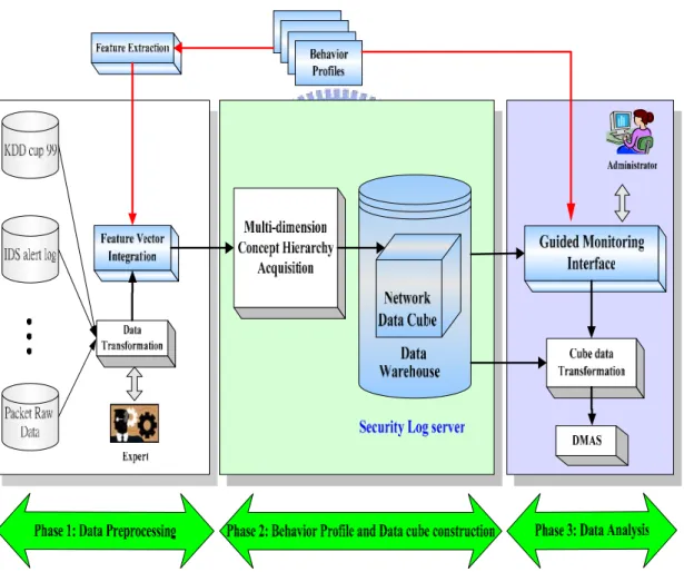
(21) Chapter 3: The Framework of Network Monitoring and Analyzing System In this chapter, the framework of network monitoring and analyzing system will be introduced. The analytic functions of framework are based on Data Warehousing technology. It is flexible because senior administrators can choose the desired granularity of each dimension by themselves using their experience during analysis process. Hence, the knowledge of analyzing network behavior will be then acquired and built to help junior administrators identify suspicious network behaviors.. The system architecture of data analyzing framework which consists of three phases is shown in Figure 3.1. In the previous research [27], different data sources are integrated into an uniform format and used to construct the cube by Multi-dimension Concept Hierarchy Acquisition Algorithm. Afterward the cube constructed is analyzed without the assistance of domain knowledge. In order to reduce the effort of administrators during the analysis of network attacks, the knowledge of network behaviors should be acquired first to enhance the analyzing framework. The knowledge Acquisition for Behavior Model Construction (KABMC) is the algorithm to acquire knowledge from expert. The knowledge will be represented by behavior profiles which record characteristics of each behavior, and use them for enhancing the analyzing system. Therefore we can find some features of profiles in Feature Extraction step, and apply these features in analyzing framework such as measurements in the fact table. For the propose of applying acquired knowledge, multiple data sources are collected and integrated with the features extracted from behavior profiles in the first phase, and then data warehouse is constructed in the. 11.

(22) second phase based upon the feature vector generated from the first phase in order to provide On-Line Analytical Process (OLAP), which could provide different granularity level for various analysis purposes. Moreover, the acquired network behavior model will be used to pre-construct data sets for efficiently analyzing several network behaviors without loosing the advantage of concept hierarchies. Finally, administrators can analyze data based on Guided Monitoring Interface (GMI) with pre-generated behavior data sets, then select interesting data for further analysis such as data mining.. Figure 3.1 The System Architecture of Data Analyzing Framework. 12.

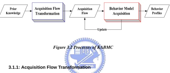
(23) 3.1:Knowledge Acquisition for Behavior Model Construction In order to enhance the analyzing ability of original system, knowledge of network behaviors needs to be acquired first. Knowledge Acquisition for Behavior Model Construction (KABMC) is used for acquiring network behavior model from experts based upon the Piaget’s Cognitive Develop Theory. There are two steps in the KABMC, as shown in Figure3.2 :. Figure 3.2 Processes of KABMC. 3.1.1: Acquisition Flow Transformation Before starting to acquire the behavior model from experts, expert’s effort could be reduced based upon prior knowledge. Then the maintenance of knowledge based on Piaget’s theory would perform knowledge development which is the same with human beings. In order to transform the prior knowledge of network specifications such as RFCs and TCP/IP 4 layers model to fit our use, we first propose the Acquisition Flow Transformation Algorithm, which will be described in detail in Chapter 4, to generate an initial acquisition flow as the basic knowledge model for modeling network behaviors in knowledge acquisition. The acquisition flow which represents the knowledge model of network behaviors will give experts choices in the behavior modeling process. This is better than ask experts to directly model a behavior without giving any information since there is a guide provided by acquired. 13.

(24) knowledge model. Then the knowledge of each network behaviors could be acquired from expert using the initial acquisition flow.. 3.1.2: Behavior Model Acquisition In this phase, the initial acquisition flow which represents knowledge will be applied to ask the expert characteristics of each network behavior. By the Self-regulation process in the Cognitive Development Theory proposed by Piaget, human beings develop knowledge based on assimilation and accommodation. In the Behavior Model Acquisition algorithm, new behaviors are first modeled with the acquired knowledge model by applying the concept of knowledge assimilation. Since the initial domain knowledge represented by acquisition flow is not enough to cover every behavior which is out of the original knowledge concept, the knowledge accommodation is then performed to update the original knowledge model. In knowledge accommodation process, the acquisition flow is updated while the knowledge is enhanced, and then the updated flow could be used in the next behavior model acquisition process.. Behaviors are modeled and the corresponding behavior profiles are generated according to the Behavior Model Acquisition Algorithm described in Section 4.2.1. After obtaining behavior profiles, the knowledge of how to identify or find these behaviors is obtained. Therefore, the knowledge can be applied in our data analyzing framework.. 3.2: Network Monitoring and Analyzing System Because the behavior profiles have be obtained, they can be used to enhance the data analysis architecture for assisting administrator to analyze network traffic. 14.

(25) 3.2.1: Data Preprocessing Phase Network traffic data such as data set in KDD cup 99, Snort alert log, etc. from every monitored host are transformed into a data set. By integrating different network traffic data, we can obtain more information. In this phase, different formats of network traffic data can be integrated into an uniform format network traffic data. Data transformation mechanism outputs a feature vector integrated from different data sources. This feature vector will be integrated with the additional features extracted from behavior profiles at the Feature Vector Integration step described in Section 5.1. The integrated feature vector will be transmitted to the data warehouse for constructing data cube.. 3.2.2: Concept Hierarchy and Data Warehouse Construction Phase After multiple data sources are integrated, a large data set which however is a flat data resource can be analyzed to obtain information behind the value in network abnormal status analysis. For example, if a host without any popular service has outbound traffic of 100,000 packets per second, it may be treated as a host generated “very large traffic” in a short period. In most environments, it is abnormal due to the distributed denial of service (DDoS) attacking signature. If the knowledge of network environment can be abstracted from domain experts by a systematic Knowledge Acquisition process, concept hierarchy of each feature of the integrated complete data source can be used to show more meaningful information. Analyzing network traffic data from different concept levels in different viewpoints will get more interesting results by monitoring network behaviors. Therefore, constructing concept hierarchy for the integrated network traffic will make network analysis result more meaningful.. A Multi-Dimension Concept Hierarchy Knowledge Acquisition (MDCHKA) 15.

(26) algorithm is proposed by previous research [27] to obtain concept hierarchies of each dimension for network traffic data from domain expert. With the concept hierarchy, integrated network traffic data can be transformed into a data cube on OLAP server. OLAP server offers many operations for us to analyze data from different dimension and concept level. Administrators can roll up or drill down the concept level for further analysis.. 3.2.3: Data Analysis Phase Guided Monitoring Interface (GMI) assists administrators in analyzing the data cube for monitoring anomaly status caused by network intrusion. With a transformation procedure, administrators can export data from data cube to some data mining tools, such as DMAS[3]. Using Data Mining techniques, administrators can get more analyzed result of network intrusion.. There is a huge amount network traffic data stored in the data warehouse. Network traffic data has the characteristic of high dimensionality. Because of containing many dimensions and concept levels, network traffic cube becomes very complicated. In order to offer administrators a systematic and efficient way to analyze data cube, GMI let administrators choose the desired dimensions and corresponding concept levels. Previous research [27] guided administrators to generate meta-data of abnormal network status. But the generated meta-data is dependent on the experience of administrators. In other words, if an administrator wants to obtain useful information from huge amount of data, he/she needs to have domain knowledge to manipulate analysis tools. Since behavior profiles are obtained before applying data analyzing framework, behavior profiles which represents domain knowledge could be used to enhance GMI. The administrator can directly manipulate GMI against 16.

(27) particular data set identified by behavior profile. GMI then transforms the meta-data into a real data cube query language, and shows administrators the data exported from data cube. Therefore, the enhancement of GMI by behavior profiles can reduce administrators’ effort or the threshold of domain knowledge they need. When abnormal network status is noticed by administrators, network traffic cube data are transformed into files which DMAS can read. Therefore, data mining techniques can go deep into data and get more analysis results.. 17.

(28) Chapter 4: Knowledge Acquisition for Behavior Model Construction In order to reduce the expert’s effort during the analyzing process, knowledge of analyzing behavior from traffic data need to be embedded in the analyzing framework. Therefore the relationship between behaviors and traffic raw data need to be acquired first. We purpose a mechanism to build a knowledge acquisition tool which imitates human beings to develop knowledge based up Piaget’s concept of knowledge development of human beings. The network behavior models which record the characteristics of raw data could be constructed by the knowledge acquisition tool.. There are two algorithms in the Knowledge Acquisition for Behavior Model Construction. First the initial acquisition flow could be obtained from Acquisition Flow Transformation algorithm based upon RFCs and TCP/IP network model. Afterward, the initial acquisition flow is used to acquire behavior models from experts in Behavior Model Acquisition algorithm. Besides, after obtaining each behavior profiles, hierarchical relations between behaviors could be identified by a simple criteria.. 4.1:Acquisition Flow Transformation Before starting to interactive with experts, expert’s effort could be reduced based upon domain knowledge. Besides, if the interaction is provided with professional sense, experts may feel comfortable during the knowledge acquisition process. Therefore basic domain knowledge needs to be obtained first.. 18.

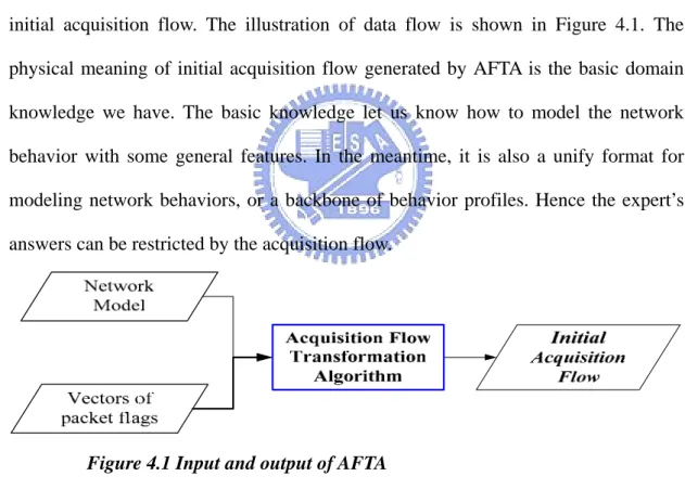
(29) In network data analysis, the first step is the packet process. The process step is generally defined by some specification such as network layers model or Request For Comment (RFC). Hence, we use the network model and features defined in the RFCs as the basic domain knowledge. Because experts are asked for helping us model network behaviors, and the possibility of human answer is hard to estimate, so we should provide some constraints to limit the range of experts answer.. The acquisition flow is used for adding some constraints in modeling process. We propose an Acquisition Flow Transformation Algorithm (AFTA) to generate an initial acquisition flow. The illustration of data flow is shown in Figure 4.1. The physical meaning of initial acquisition flow generated by AFTA is the basic domain knowledge we have. The basic knowledge let us know how to model the network behavior with some general features. In the meantime, it is also a unify format for modeling network behaviors, or a backbone of behavior profiles. Hence the expert’s answers can be restricted by the acquisition flow.. Figure 4.1 Input and output of AFTA. If the feature of a network behavior behaves at low network layer, the behavior can be discovered at early stages of processing packet. So if the network behavior can be differenced at lower layer, the cost is lower than identifying the behavior at higher layer such as application layer. Therefore, the features in the acquisition flow are ordered from bottom to the top network layer. 19.

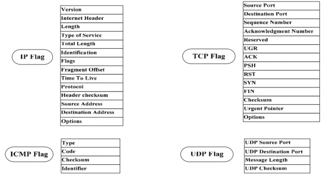
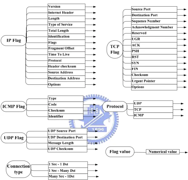
(30) 4.1.1: Acquisition Flow Transformation Algorithm The algorithm for generating initial acquisition flow is shown as follows. Algorithm 1 : Acquisition Flow Transformation (AFT) Algorithm Input:. Vectors of packet flags of protocol specifications such as RFCs TCP/IP 4 layers model. Output: Initial Acquisition Flow Step 1:. Step 2: Step 3:. Step 4: Step 5: Step 6:. Create attributes named with protocol name and “flag” Step 1.1 Scan the corresponding vector of flags to obtain the attribute values. List other attributes which has a mapping to network model and corresponding attribute values. create sub flows Step 3.1: represent each attribute by a node Step 3.2: represent the corresponding attribute values by the edges directed from its attribute node Sort the attributes by the network protocol layers from bottom layer to top layer. Identify the dependency relation of each attributes. generate the acquisition flow Step 6.1: Start from the first attribute, Step 6.2: for each edges, find if there is any attribute dependent with the value Step 6.2.1: If Found, append the sub flow of the attribute at the end of the edge. Step 6.2.2: Else append the sub flow of the next attribute at the. Example: Generating initial acquisition flow according to AFT The input vector of flags is from RFC 791 (IP), RFC 792 (ICMP), RFC 793 (TCP) and RFC 768 (UDP). Step 1: Create attributes named with protocol name and “flag”. 20.

(31) Figure 4.2 Flag attribute and corresponding values Step 2: List other attributes which has a mapping to network model and corresponding attribute values.. Figure 4.3 More attribute and corresponding values after step2. 21.

(32) Step 3:. Create sub flows Step 3.1: represent each attribute by a node Step 3.2: represent the corresponding attribute values by the edges directed from its attribute node. Figure 4.4 Sub flows of each attribute Step 4: Sort the attributes by the network protocol layers from bottom layer to top layer. Table 4.1 Attribute order after sorting Order. Attribute. 1. Connection Type. 2. IP Flag. 3. Flag value. 4. Protocol. 5. TCP flag. UDP flag. 22. ICMP flag.

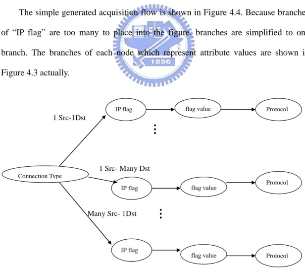
(33) Step 5: Identify the dependency relation of each attributes. Attribute values of “Protocol” are TCP, UDP and ICMP. There has corresponding attribute with these values at next node. Therefore, the dependent relation is shown in Table 4.2: Table 4.2 Table of corresponding dependent relation Attribute values of “Protocol”. Corresponding dependent attribute. TCP. TCP flag. UDP. UDP flag. ICMP. ICMP flag. Step 6: Generate the acquisition flow. The simple generated acquisition flow is shown in Figure 4.4. Because branches of “IP flag” are too many to place into the figure, branches are simplified to one branch. The branches of each node which represent attribute values are shown in Figure 4.3 actually.. flag value. IP flag. Protocol. 1 Src-1Dst. … 1 Src- Many Dst Connection Type flag value. IP flag. …. Many Src- 1Dst. Protocol. IP flag. flag value. (a) Generated acquisition flow until attribute “Protocol” 23. Protocol.

(34) Connection Type. 1 Src-1Dst. Many Src- 1Dst. 1 Src- Many Dst. IP flag. IP flag IP flag. …. IP Flags flag value. flag value. Protocol. Protocol. …. Protocol. TCP. …. TCP Flags. …. …. ICMP. UDP. TCP flag. flag value. UDP flag. UDP Flags. ICMP flag. …. ICMP Flags. …. (b) Generated acquisition flow with dependent relation of values of “Protocol” Figure 4.5 Generated Acquisition Flow. The above example shows how to generate the initial acquisition flow by the AFTA algorithm. After the initial acquisition flow is generated, basic knowledge to help experts to model the network behavior is obtained. Therefore, we can start to acquire behavior models from experts.. 4.2:Behavior Model Acquisition Behavior Model Acquisition is the main process of knowledge construction. The knowledge construction process is based on Piaget’s schema theory, which is well known theory in developmental psychology. Piaget insisted that human development 24.

(35) of cognitive system is based on a Schema System. Schema is a module of human cognitive system. He believes that our cognitive system is formed through interacting with many things around us after the birth. The fundamental mechanism underlying the above forming process consists of the two phases: assimilation and accommodation. Assimilation involves putting information into an existing scheme without changing the scheme. Accommodation is the process of changing our existing scheme in order to make new, non-compatible information fit our understanding. In accommodation, our understanding or problem solving ability is improved. Therefore, the knowledge development process of human beings is based on the assimilation and accommodation.. The cognitive schema in our mechanism is the acquisition flow. The knowledge acquisition tool maintains the acquisition flow based on the assimilation and accommodation. Assimilation here is that information of network behavior is inputted following the acquisition flow. Accommodation here is in the form of updating acquisition flow. Besides, it still needs a way to obtain the information of network behavior model, acquisition process, and Therefore, a Behavior Model Acquisition Algorithm (BMAA) is proposed here for interacting with experts to finish these two phases.. Besides, there is another reason to need the initial acquisition flow. If experts are asked for helping us model the network behaviors without providing related information, experts are hard to model the behavior and the acquired models may be different because of different experts. Hence, the initial acquisition flow introduces in previous sub section is utilized for the reason. The initial acquisition flow represents basic domain knowledge which is used for leading experts’ answers to unify format 25.

(36) during the behaviors modeling process. Hence, the Behavior Model Acquisition Algorithm (BMAA) models network behaviors from experts using Acquisition Flow. The illustration of data flow is shown in Figure 4.6. In the BMAA, knowledge engineers have no need to involve in because of acquisition flow. Therefore, we can build a knowledge acquisition tool applying the BMAA, experts then help us model the network behavior using the tool. Without involvement of knowledge engineers, experts can model behaviors freely at any time in his leisure.. Figure 4.6 Input and Output of BMAA. Because the knowledge we have initially is basic, the ability of modeling behavior using the basic knowledge may be not enough. The initial acquisition flow represents how to differentiate or model the object, but it may reach its limit soon as long as the number of kinds of behaviors continued increases. The help of reducing the expert’s effort is also not enough. Hence we need to enhance the knowledge to decrease the times of this situation. Thus knowledge accommodation is needed. If we. 26.

(37) want to differentiate more behaviors, we need more attributes in our knowledge. So the expert is asked for additional attributes when two behaviors can not be differentiated following acquisition flow. This is the process of knowledge accommodation. The original acquisition flow is also updated. The physical meaning of updating flow is enhancing the knowledge embedded in the tool. At next round, expert models behavior using updated flow.. When experts model behaviors using our tool, it lists attribute and corresponding values for choosing. Therefore, if the behavior is not out of scope of original knowledge very much, experts almost do the confirmation process. Else we ask experts for new attributes to enhance the knowledge. Hence we can save experts’ effort as more as possible based on our knowledge. The detail of the BMA algorithm will be shown in the next sub section.. 4.2.1: Behavior Model Acquisition Algorithm In this section, we will show how Behavior Model Acquisition Algorithm works. Examples are shown after the algorithm.. Algorithm 2: Behavior Model Acquisition (BMA) Algorithm Prior knowledge: Acquisition Flow Input: behavior descriptions Output: behavior profiles Function: Update_Flow() { Update the original acquisition flow. }. 27.

(38) Function: Knowledge Assimilation (type,v) { Switch (type) { Case “value”: Go to the branch directed by the value v. Case “node” : Add a node filled behavior name v at the end of the edge } } Knowledge Accommodation(type, Z) { Switch (type) { Case “value”: Add an edge from current node which has the value Z. Case “node” : Replace the original behavior node by the attribute node with name Z. Default: Add two behavior nodes named } } Confirm_Detail() { ask expert if there are another characteristics of raw data step 1: Ask expert to represent each characteristics in the form of attribute and attribute value step 2: ask expert to confirm if this attribute is dependent with some previous attribute values. Step 3: represent them in the form of the node and edge. Step 4: Insert the node and edge between the behavior node and its parent Step 5:call Update_Flow() }. 28.

(39) Step1:for each behavior select one behavior description, start from the first node of Acquisition Flow Step1.1: ask the expert following things until reach one of the end nodes of Acquisition Flow 1.1.1:ask the attribute value of the behavior from expert 1.1.1.1:there has a suitable value X, call Knowledge Assimilation (value,X) 1.1.1.2:else select one case z. Case 1:has more than 1 suitable value . Call Knowledge Accommodation(value, all. z. suitable value) Case 2:don’ care. z. Call Knowledge Accommodation(value, X) Case 3:add new attribute value W. Call Knowledge Accommodation(value, W) 1.1.1.3: append the sub flow which has the same rest of attributes at the next level with the new edge from the current node. call Update_Flow(). 1.1.2: if the node is not the last attribute node, go to 1.1.1 Step 1.2: if there is a node at the end which is a behavior node, then go to Step 1.4 Step 1.3:, call Knowledge Assimilation (node, behavior name), call Update_Flow(). Return for this behavior. Step 1.4: ask expert a new attribute to differentiate the two behaviors, Call Knowledge Accommodation (node, attribute name) Step 1.5: ask expert the corresponding values of the new attribute of two behaviors, if the value is a and b for original behavior and the behavior now, respectively. Call Knowledge Accommodation (value, a), Call Knowledge Assimilation (node, original behavior name), Call Knowledge Accommodation (value, b), Call Knowledge Assimilation (node, current behavior name), Call Update_Flow(). Step 1.6: If there has un-processed behavior description, go to step 1 Step2: If experts want to confirm the detail description for each attributes, Call Confirm_Detail() z reason: the attribute for now is enough to differentiate all incoming behaviors, but may not be able to describe the behavior in detail 29.

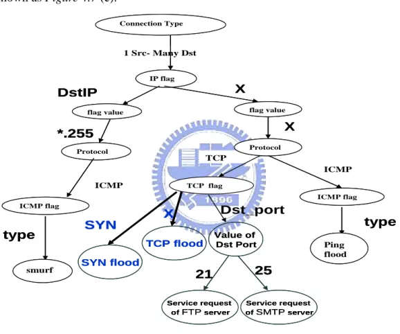
(40) Step 3: Trace the Acquisition Flow, from each behavior leaf node, along its parent to the first attribute node, we can get the profile of each behavior. Step 3.1: Obtain each attribute, attribute values and dependent relations for the behavior in the traverse. Step 3.2: Start at the first attribute. Generate the profile table. For each attribute, if there is no dependent relation with previous attribute value, go to Case 1, else go to Case 2. Case 1: Add a new row with two columns filled with attribute and attribute value respective. Case 2: . Split the cell at the last row and column into 3 columns. Fill the value in the order of previous attribute value (in original cell), attribute, attribute value.. The initial acquisition flow used in. Connection Type. the following example is shown in 1 Src- Many Dst. Figure 4.5. When there is a behavior IP flag. need. to. be. modeled,. DstIP. knowledge. flag value. assimilation is executed first. Attribute. X flag value. X. *.255 and corresponding values are listed from the. first. attribute. following. Protocol. Protocol. the. ICMP ICMP. acquisition flow. Experts then choose. ICMP flag ICMP flag. suitable values of the behavior step by. type. type Ping flood. step. The chosen attribute values has a smurf. corresponding directed edges, follow the edges we can have a path. Finally, we add. Figure 4.7 Smurf and Ping flood. the behavior node at the end of the path.. 30.

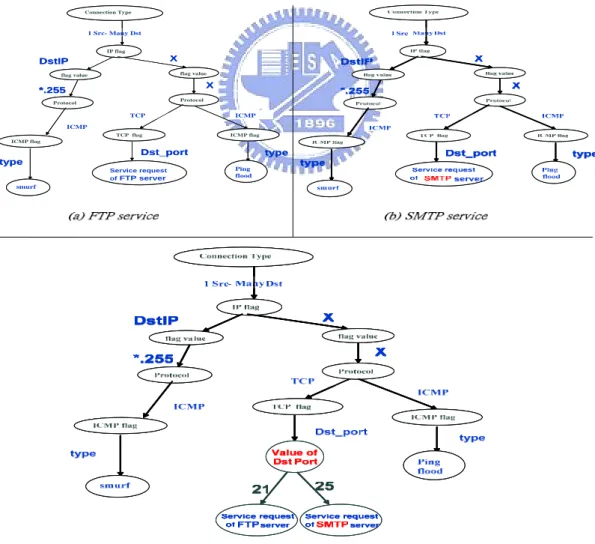
(41) Figure 4.7 shows the results of knowledge assimilation. The result path of Smurf attack which generated ping flood to broadcast address is shown as the left part of Figure 4.7. Other branches which are not chosen in the acquisition flow are omitted in Figure 4.7. Next behavior needed to be modeled is ping flood which generates huge amount of ICMP ping packets. When experts want to select a suitable value of “IP flag” of ping flood behavior, expert thinks that there is not a feature of ping flood appeared in the IP layer; therefore expert select case 2 of step 1.1.1.2. Things do by case 2 is adding a edge from current node which has a mark “X”. The same situation also happened at the attribute “flag value”. The result path of ping flood is shown as the right part of the figure 4.7.. Connection Type. 1 Src- Many Dst IP flag. X. DstIP. flag value. flag value. X. *.255 Protocol. Protocol. TCP. ICMP. ICMP TCP flag. ICMP flag. ICMP flag. Dst_port. type. type Service request of FTP server. Ping flood. smurf. Figure 4.7 FTP and SMTP 31.

(42) Fig. 4.8 is an example of knowledge accommodation. Figure 4.7(a) is the result of knowledge assimilation of FTP server behavior. Figure 4.7(b) is the original result of knowledge assimilation of SMTP. But the tool will find that there is a behavior node (FTP) in the same position, so it is the time to perform knowledge accommodation. Experts is asked for a new attribute and corresponding values to distinguish two behaviors. Hence, the result after knowledge accommodation is shown as Figure 4.7 (c). Connection Type. 1 Src- Many Dst IP flag. X. DstIP. flag value. flag value. X. *.255 Protocol. Protocol. TCP ICMP. ICMP. TCP flag ICMP flag. ICMP flag. Dst_port. X. type. SYN. type. Value of Dst Port. TCP flood. smurf. SYN flood. 21 Service request of FTP server. Ping flood. 25 Service request of SMTP server. Figure 4.8 After adding SYN flood and TCP flood. Figure 4.8 is the result after adding SYN flood and TCP flood. After all network behaviors are modeled follow the acquisition flow. Experts can decide if they want to add more detailed description of some behaviors. If experts decide to do so, more detailed information will be acquired in the form of attribute and attribute values. The additional attribute and corresponding values will be represented in the form of node and edge, and be inserted into the acquisition flow, as shown in Figure 4.9. 32.

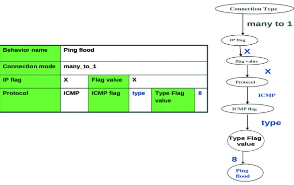
(43) Connection Type. 1 Src- Many Dst IP flag. X. DstIP. flag value. flag value. X. *.255 Protocol. Protocol. TCP ICMP. ICMP TCP flag. ICMP flag. ICMP flag. type. X. SYN. Type Flag value. SYN Flag value. 8. Dst_port type Value of Dst Port. TCP flood. 25. 21. 1. smurf SYN flood. Service request of FTP server. Type Flag value. 8. Service request of SMTP server. Ping flood. Figure 4.9 More detail of each behavior Finally, behavior profiles have to be generated. Back trace the acquisition flow from a behavior node, we then get each attribute value of the behavior. Because of Step 1.1.1.1 and Step 1.1.1.2, we ensure that there is only one path from the first attribute node to a behavior node. Behavior profiles are generated as a table consisting of obtained attribute and attribute values. Connection Type. many to 1 IP flag. Behavior name. Ping flood. X flag value. Connection mode. many_to_1. IP flag. X. Flag value. X. Protocol. ICMP. ICMP flag. type. X Protocol. Type Flag value. 8. ICMP ICMP flag. type Type Flag value. 8 Ping flood. Figure 4.10 The Behavior profile of ping flood 33.

(44) The behavior profile of ping flood is shown in Figure 4.10. Attributes with dependent relation are in the same raw such as “IP flag” and “Flag value”.. 4.3:Hierarchical relation between behaviors There are some hierarchical relations between network behaviors, if the relations can be found. It can be used to reduce the effort on the query process when querying the same type behaviors. We compare each two behavior profiles which record the characteristics of the behavior to find out relations. The hierarchical relation defined here is named by “is a” relation. There are some meanings could be represented by “is a” relation, such as “is a kind of”, “is a part of”, and “is a component of”, etc. The relation here is used to represent “is a subset of”. If there are two behaviors A and B, the hierarchical relation is identified in the following situation: z B is a subset of A if the following condition is true ‧ The same connection type and protocol ‧ Attributes are the same, and only one attribute or one kind of dependent attributes value is different. And to that attribute, If B has a specific value and A is don’t care. For instance, take the result shown in Fig. 4.7 as an example. It can be found that the Smurf attack and ping flood have the same value of connection type and protocol. The only difference between these two behaviors is the characteristic of IP. Because of the condition mentioned above, Smurf attack is a sub set of ping flood since Smurf attack has more one constraint that destination IP is broadcast address. Hence, there is a hierarchical relation between Smurf attack and ping flood. Other hierarchical relations are shown in Fig 4.11, which are the relations between 9 common DDoS attacks. 34.

(45) Is a UDP Flood. Ping flood. Tcp Flood. ACK flood. behavior. SYN flood. Fraggle. Figure 4.11 Hierarchical relations between DDoS behaviors. 35. smurf.

(46) Chapter 5: Building the Network Monitoring System After acquiring behavior profiles, we start to run data analysis framework. The framework is shown in Figure 3.1. Because we have obtained the domain knowledge of network behaviors form experts, some enhancement can be used to improve the framework.. 5.1:Feature Vector Integration Because of adopting different network traffic data format, different researches use different methods and have different analysis results. For taking advantages of different analytical methods, integration of multiple data sources is a very important procedure. Multiple data sources contain different data formats, so they need to be preprocessed and transformed to an integrated data with a common data format.. Two algorithms shown below are purposed in [27] to integrate different data sources: z. Multi-Source Data Format Integration (MSDFI) Algorithm: The concept of a new data source is generalized to the connection level first. If the concept of the new data source is already at connection level, the generalization is omitted. Second, features with different types of new data sources are added into the integrated data source. At last, the integrated data format can be used to merge multiple network traffic data sources.. z. Data Source Transformation (DST) Algorithm:. It shows how to integrate. multiple network traffic data sources according to the integrated data format that MSDFI algorithm generated.. 36.

(47) After DST process, we get a feature vector. There are also some features can be identified in behavior profiles. They will be integrated to generate a new feature vector. A simple process of feature vector integration is described as follows. Some notation is defined before the description. z. F : a temporal feature set. z. f : a feature. z. FV: the feature vector generated by DST.. First, features need to be identified from behavior profiles. If an attribute has a specific numerical value, then add a feature f named by “behavior_name count” in a temporal feature set F, and the attribute has a specific numerical value is the condition of the corresponding feature. Second, integration of the temporal feature set F and the feature vector FV is executed. For each feature f in the F, if f is not in FV, than add f in FV.. Take the “Ping flood” for an example, as shown in Fig 4.10. The condition: “type=8” could be found. After identifying the features, they are integrated into the original feature vector generated by DST. In data warehouse, fact table is the place where network traffic integrated data are stored. Network raw data are transformed into connection feature vectors in Data Transformation, and then integrated with features identified from behavior profiles. The integrated feature vectors are stored in fact table without generalization or aggregation. The format for fact table is the same as feature vector mentioned in Data Preprocessing Phase. Some field is related to dimension table and others are measures. In fact, features identified from behavior profiles are measurement in the fact table. The illustration about format of Network Traffic Fact Table is shown in Table 5.1.. 37.

(48) Data fields. SrcIP. Table 5.1 Fact Table. DstIP Type … Num. measurements. Flow. Ping_Count …. 5.2:Concept hierarchy and Data warehouse construction If network traffic concept hierarchies for integrated data source are constructed by Knowledge Acquisition process, the integrated network traffic data can be analyzed in different concept level. For example, the behavior of a host can be evaluated by analyzing IP dimension in IP-address concept level; however, behaviors of a subnet can be evaluated by analyzing network traffic in class-c concept level after concept hierarchies are constructed. With constructing concept hierarchies and data cube, evaluating behaviors in every concept level of IP dimension is natural because of roll-up and drill-down operations that OLAP server offered. Without constructing concept hierarchies and data cube, administrators have to search manually for network traffic data of a subnet from a flat data source for evaluating behavior of a subnet. Analyzing network behaviors on every concept level of every dimension would become easier with the assistance of the constructed concept hierarchies and data cube.. 5.2.1: Concept Hierarchy Construction Here, Dimension Concept Hierarchy Knowledge Acquisition (DCHKA) algorithm proposed in [27] is used to construct concept hierarchies. The input of 38.

(49) DCHKA is the feature vector format generated in Data Preprocessing Phase. Concept hierarchy is constructed from bottom to top because the original data collected in previous phase are based on the lowest concept level. Experts are guided to generalize concept from lower concept level to higher level and to define the mapping relations between values appearing in lower concept level and higher concept level. Repeat the steps in DCHKA algorithm for each dimension in the feature vector format and a concept hierarchy would be constructed at last. An example of constructed concept levels is shown in Figure 5.1. With the help of expertise in the form of concept hierarchy, behaviors in different concept level can be evaluated and analyzed. Time Dimension. Source IP Dimension. Destination IP Dimension. Day. ClassA. ClassA. Alert Dimension. Hour. ClassB. ClassB. Priority. Minute. ClassC. ClassC. AlertClass. Second. IP Address. IP Address. Alert. Figure 5.1 Concept levels of each dimension of network traffic data. 5.2.2: Data Warehouse Construction After constructing dimension concept hierarchies, data cube schema need to be selected in order to build network traffic data cube. The most common modeling paradigm is the star schema, in which the data warehouse contains (i) a large central table (fact table) containing the bulk of the data, with no redundancy, and (ii) a set of smaller attendant tables (dimension tables), one for each dimension. The schema graph resembles a starburst, with the dimension tables displayed in a radial pattern around the central fact table. In network traffic data, star schema is the most suitable schema for the relation between raw data and concept hierarchies. 39.

(50) The steps after selecting data cube schema are selection of dimensions and measurements from fact table. An example of dimensions has been shown in Figure 5.1. Features which are used to evaluate behaviors can be chosen to be measures. In network traffic data, feature such as Packet Number, Packet size, Connection Number, Number of Ping packets, Number of SYN packets, etc. are chosen to be measures. Measures are aggregated when concept level is generalized from low concept level to higher concept level. Therefore, network behaviors can be evaluated by measures from different dimension. For example, total packets size can be used to evaluate behavior of a host or a subnet. Following the steps mentioned above, a star schema as shown in Figure 5.2 of network traffic data cube can be constructed.. Figure 5.2 : Cube schema for constructing data warehouse. 40.

(51) 5.2.3: Dimension Table Maintenance Dimensions in network traffic data have the characteristic that the number of values in each concept level is large. For example, the number of all possible values of IP addresses is 256*256*256*256, but only tiny fragment which ranges from thousands to ten thousands will appear in our network traffic data. It is wasted and impossible to maintain all IP addresses in Source IP dimension table or Destination IP dimension table. Only IP addresses which communicate to monitored hosts are maintained in dimension table. When a new IP address appears, the new IP address is added into dimension table and the corresponding higher concept level value is confirmed. If the higher concept level value of the new IP address does not exist in dimension table either, new higher concept level value is added. As time goes on, the size of dimension table becomes very large so that a proper method to decease the size of dimension table such as deleting the IP addresses that do not appear for a long time is needed.. Other dimensions such as Alert and Port have the similar characteristic. It is unnecessary to store values that never appear or not appear for a long time in network traffic data into dimension tables. This will cause the low performance of OLAP server because of dispensable join time and query time. So dimension tables with this characteristic should be adjusted dynamically for higher system performance.. 5.3:Data analysis In the original framework, administrators need to construct the meta-data, then use it to find the interesting data set. This process of constructing meta-data needs administrator manipulate the Guided Monitoring Interface (GMI) manually, and the 41.

(52) result of interesting data set is highly dependent on how much domain knowledge that administrators have. In order to reduce the administrators’ effort, we use behavior profiles to enhance the original GMI. Behavior profiles which represent the domain knowledge can be used to generate a part of meta-data.. Figure 5.3 Comparison between original and enhanced workflow. The comparison between original framework and enhanced one is shown in Figure 5.3. As mentioned above, in the original workflow, cube meta-data was constructed according to the requirement of administrators hinted by Cube Meta-data Construction Algorithm (CMCA). In the enhanced workflow, the acquired behavior profiles can be used to select behavior data form the original huge cube. The general process step of CMCA is shown in Figure 5.4. The CMCA is just a general guide for manipulate GMI, but the detailed decision during CMCA is highly 42.

(53) dependent in the experience of administrators. Therefore suspicious network behaviors may not be able to identify as soon as possible by a junior administrator. Because the domain knowledge have been acquired as behavior profiles. Knowledge of which dimension should be chosen and which specific value should be monitored for the corresponding behavior is record in the behavior profiles. Hence, we can use the behavior profile to reduce analyzing effort of administrators, especially junior ones.. Figure 5.4 General process step of CMCA. As mentioned above, the first and the third step in Figure 5.4 could be done by the support of domain knowledge. Therefore the administrators’ effort could be reduced.. 5.3.1: Behavior model Transformation In order to directly choose the data of network behaviors from database or data warehouse, data query needs to be generated. Since we have the knowledge of network behavior models, it can be used to generate data queries. Here we propose a process to transform the behavior profiles to the corresponding data queries. As shown in Algorithm 3. 43.

(54) Algorithm 3: Behavior Model Transformation Algorithm Input: Behavior Profiles Output: Data Query Step 1: Generate the main part of data query. Depend on the value V of attribute “connection type”, generate the corresponding query as below: Switch(V) { Case “1_to_1” : Query =. Select SrcIP , DstIP From traffic record. Case “Many_to_1 [X]” : Query =. Select DstIP , count(DISTINCT SrcIP) From traffic record Group by DstIP Having count(DISTINCT SrcIP) > X. Case “1_to_Many [X]” : Query =. Select SrcIP , count(DISTINCT DstIP) From traffic record Group by SrcIP Having count(DISTINCT DstIP) > X. } Step 2: Choose the data source according to the protocol of the behavior traffic record = protocol traffic data Step 3: Add the constraint into the query z Flag constraint ‧ Add condition in“where” clause z Threshold constraint ‧ If no word “DISTINCT” appears in the constraint ‧ If connection mode is. many_to_1. ‧ add count(SrcIP) as behavior count in“select＂ clause ‧ Add thresholds of count(SrcIP) in the“Having＂ clause ‧ If connection mode is 1_to_many ‧ Add count(DstIP) instead of count(SrcIP) ‧ else ‧ Add count(DISTINCT Flag_name) as behavior count in “select” clause ‧ Add thresholds of count(DISTINCT Flag name) in the ”Having” clause 44.

(55) Take the behavior profile shown in Figure 4.10 for an example. The connection type of ping flood is “many_to_1”, and suppose the default threshold of “many” is X. (How many source IPs connect to a Destination IP could be treated as suspicious behavior? X is the threshold of number of distinct source IPs.) The protocol used in ping flood is “ICMP”, and the constraint of ping flood is that for every packet in the ping flood, the value of flag “Type” is 8. Moreover, administrators can set the threshold of the amount of ping packets to be treated as a ping flood. Hence, the corresponding data query is shown as follows: Select DstIP , count(DISTINCT SrcIP), count(SrcIP) as Ping Flood Count From ICMP traffic record Where type=8 Group by DstIP Having count(DISTINCT SrcIP) > X. and count(SrcIP) >y. A simple result of the above query is shown in Table 5.2 , when X=50 and Y=1000000. Table 5.2 The result of data query DstIP. # of SrcIP. Ping flood count. 10.113.87.175. 58. 1000670. …. …. …. 45.

(56) 5.3.2: Hierarchical relation After acquiring network behaviors, hierarchical relations could be identified from behavior profiles. Hierarchical relations are identified by checking if one behavior has more detail constraint than the other which has the same values of connection type and protocol in the behavior profile, as mentioned in section 4.3. The relation could be used to reduce the effort of data query.. Figure 5.5 original data query and enhanced one. Hierarchical relation between two network behaviors could be used to simplify the data query of the behavior which is the subset in the relation. Suppose that two monitored behaviors A and B with a hierarchical relation between them, B is a subset of A. Data set of A could be looked up by the corresponding data query generated by 46.

(57) Algorithm 3. Afterward the data query of behavior B could be reduced by looking up data from data set of A. The constraint in the data query of B is just the additional constraints which not appeared in the behavior profile of A. As shown in Figure 5.5, without the hierarchical relation, data set B is queried from huge data cube by the original data queries. After knowing the hierarchical relation, data set of b could be looked up form data set A. Thus the time of looking up data set B using the reduced query is shorter, because data set A is much smaller than original data cube. For example, Smurf flood is a subset of ping flood. Without knowing this hierarchical relation, the corresponding data queries of the two behaviors are shown below: I.. Data query of ping flood: Select *, count(DISTINCT SrcIP), count(SrcIP) as Ping Flood Count From ICMP traffic record Where type=8 Group by DstIP Having count(DISTINCT SrcIP) > X and count(SrcIP) >y. II.. Data query of Smurf flood: Select *, count(DISTINCT SrcIP), count(SrcIP) as Smurf Flood Count From ICMP traffic record Where type=8 and DstIP like ‘%.255’ Group by DstIP Having count(DISTINCT SrcIP) > X. and count(SrcIP) >y. After knowing that Smurf flood is a sub set of ping flood, the data query of Smurf flood could be simplified after data set of ping flood has be queried out. The modified data queries are shown as follows: I.. Data query of ping flood: Create view Ping Flood record Select *, count(DISTINCT SrcIP), count(SrcIP) as Ping Flood Count From ICMP traffic record 47.