Finite analytic model for flow and transport in unsaturated zone

F

INITE

A

NALYTIC

M

ODEL FOR

F

LOW AND

T

RANSPORT

IN

U

NSATURATED

Z

ONE

By Whey-Fone Tsai,

Tim-Hau Lee,

Ching-Jen Chen,

Shin-Jye Liang,

and Chia-Chen Kuo

transport equations in an unsaturated zone. The finite analytic method treats the nonlinear coefficient terms of the governing equations as constants in the element so that linearized partial differential equations can be obtained and solved in each element. The accuracy and limitations of the numerical method are systematically explored. The flow and transport simulations are examined using a one-dimensional laboratory infiltration test and an analytical solution of a two-dimensional subsurface transport problem, respectively. In the advection-dominant, vertical, one-dimensional infiltration problem, nine spatial weighting schemes are proposed to evaluate the averaged unsaturated hydraulic conductivity in a discretized element. Among them, the geometric mean weighting scheme provides the most accurate results as compared with the infiltration data. In verification of the two-dimensional solute transport problem, the nine-node elements are placed in the interior domain, and different layers of five-node elements are placed at the boundaries to investigate if the numerical experiment setup was proper and the algorithm was accurate. The developed numerical model is then applied to an irregular-domain landfill leaching problem to reveal the features of subsurface transport in unsaturated zone. Numerical aspects to be further explored are suggested.

INTRODUCTION

In the subsurface, pollutant moves with water flow by several processes, including advection, diffusion, retardation, and decay. To investigate the consequence of the hazard posted by solute, it is important to look into the problems of water and solute migration in the unsaturated zone. In mathematical terms, solute transport in the subsurface is described by the advection-diffu-sion differential equation. The equations for flow and associated solute transport in the unsaturated zone along the vertical di-rection are highly nonlinear. Particularly, the nonlinear coeffi-cient terms are functions of the dependent variables and are very sensitive to the dependent variables. During infiltration, the large gradients of pore pressure and hydraulic conductivity make the numerical simulation in an unsaturated zone even more difficult. The accuracy of numerical solutions may be de-teriorated if an improper numerical algorithm is used.

Recently, a nontraditional, analytical-solution based numeri-cal technique named the finite analytic method (Chen and Chen 1984a,b; Chen 1989) has attracted various researchers in the environmental engineering community (Hwang et al. 1985; Li et al. 1989; Tsai et al. 1993; Pi and Hjelmfelt 1994). The method combines numerical flexibility with the advantages of analytical solutions such that the truncation errors occurring in other nu-merical methods can be minimized and the nunu-merical solutions are quite stable (Zeng and Li 1987). Hwang et al. (1985) first used the finite analytic method of Chen (1989) for solving the horizontal, two-dimensional solute transport equation. In the fi-nite analytic method, the coefficients of the governing equations are frozen in each subdomain so that linear partial differential

1

Res. Sci., CFD & Envir. Engrg. Group, Nat. Ctr. for High-Perfor-mance Computing, No. 7 R&D 6th Rd., Hsinchu Science-Based Industrial Park, Shinchu, Taiwan.

2_{Assoc. Prof., Dept. of Civ. Engrg., Nat. Taiwan Univ., Taipei, Taiwan.} 3

Prof., Dept. of Mech. Engrg., Florida A&M Univ./Florida State Univ., Tallahassee, FL 32316.

4

Res. Sci., CFD & Envir. Engrg. Group, Nat. Ctr. for High-Perfor-mance Computing, No. 7 R&D Rd., Hsinchu Science-Based Industrial Park, Hsinchu, Taiwan.

5

Res. Sci., CFD & Envir. Engrg. Group, Nat. Ctr. for High-Perfor-mance Computing, No. 7 R&D Rd., Hsinchu Science-Based Industrial Park, Hsinchu, Taiwan.

Note. Associate Editor: Alexander Cheng. Discussion open until Oc-tober 1, 2000. To extend the closing date one month, a written request must be filed with the ASCE Manager of Journals. The manuscript for this paper was submitted for review and possible publication on March 8, 1999. This paper is part of the Journal of Engineering Mechanics, Vol. 126, No. 5, May, 2000.䉷ASCE, ISSN 0733-9399/00/0005-0470– 0479/$8.00⫹ $.50 per page. Paper No. 20423.

equations can be solved in each element subject to appropriate boundary conditions at the element’s boundaries. Li et al. (1989) employed the finite analytic method to the two-dimensional ir-rotational gravity flows over a spillway with a free surface. The coupled solutions of free surface level and flow rate were solved and in good agreement with experimental measurement. Pi and Hjelmfelt (1994) used a hybrid finite analytic method to solve the lateral subsurface storm flow described by the extended DuPuit-Forchheimer equation. They concluded that a four-point numerical formula could provide results that are stable and ac-curate without using small time steps. In addition to the reports indicated above, the treatment of irregular boundaries using the finite analytic method associated with mixed nine-node and five-node elements and solving the system of algebraic equa-tions on a Cartesian grid system was developed by Tsai et al. (1993) for unsaturated flow problems. One of the common as-pects among the reviewed literature was results in a matrix of a positive nature. Leonard and Mokhtari (1990) indicated that the hybrid finite analytic method is equivalent to the first-order upwinding scheme for advection with physical diffusion omitted when the Peclet number is over two, and the advantage of the finite analytic method is its property to increase the mesh Peclet number of stability.

The present study, therefore, is aimed at solving the subsur-face flow and solute transport equations in an unsaturated zone by using the finite analytic method. In an unsaturated zone, the sharp wetting front may cause large velocity gradients along the vertical direction. Hence, proper numerical manipulation is re-quired to get through the numerical difficulties associated with the sharp front capturing. Since both flow and transport in the subsurface are advection-diffusion problems, the same numeri-cal formulation can be used. Also, for the purpose of field ap-plications, we should take the irregularity of computational do-main into account in the numerical formulation. The viewpoints noted above, together with verifications, applications, and fea-tures of the numerical model, are explored in this study.

GOVERNING EQUATIONS

Vertical Two-Dimensional Subsurface Flow in Unsaturated Zone

The Richards equation (Bear 1979) describing transient, two-dimensional subsurface flow in an unsaturated zone, or unsaturated flow, is

FIG. 1. Nine-Node and Five-Node Local Elements in Domain with Irregular Boundaries

FIG. 2. Numerical Solution Procedures for Nine-Node Ele-ment: (a) in Original x-z Coordinate System; (b) Transformation from z Coordinate System to z * Coordinate System; (c) Uniform-Grid Element Used to Provide Analytical Solution

⭸H ⭸ ⭸H ⭸ ⭸H ⭸K

Cs ⫺

冉 冊 冉 冊

⭸t ⭸x ⭸x ⭸z ⭸z ⭸z

Eq. (1) assumes that air pressure is negligible and that there is no sink or source in the flow domain. The hydraulic con-ductivity in the unsaturated zone, K, is isotropic, and the po-rosity and water density in the porous media remain constant.

H = pressure head; Cs = specific moisture capacity, which is

a nonlinear function of H and is defined as⭸␪(H)/⭸H; and ␪ = volumetric water content. K and ␪ are both the nonlinear functions of H. The two functions can be determined by lab-oratory experiments. x and z = horizontal and vertical (positive upward) space coordinates, respectively; and t = time.

Vertical Two-Dimensional Subsurface Transport in Unsaturated Zone

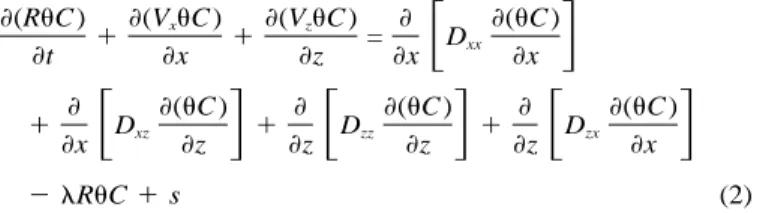
The governing equation for the vertical two-dimensional subsurface solute transport in an unsaturated zone (Bear 1979) can be written as ⭸(R␪C)_⫹⭸(V ␪C)x _⫹⭸(V ␪C)z ⭸ ⭸(␪C) =

冋

册

冋

册 冋

册 冋

册

in which C = solute concentration; R = retardation factor due to sorption of soil; Vxand Vz= porous velocity components of

unsaturated flow in the x and z directions, respectively;

Dxx, Dzz, Dxz, and Dzx = coefficients of mechanical dispersion

provided that the contribution of molecular diffusion to dis-persion is neglected;␭ = first-order decay coefficient; and s = solute source-sink term. Vx, Vz, and ␪ in (2) can be obtained

from the solution of the unsaturated flow equation, (1). Math-ematically, the dependent variable C of (2) can incorporate␪ and form a new dependent variable C* = C␪. The parameters

R, Dxx, Dzz, Dxz, Dzx, and␭ are described in the following. The

retardation factor, R, is defined as

Kd␳b

R = 1⫹ (3)

␪

in which Kd= equilibrium distribution coefficient, which is the

mass of chemical adsorbed to the solid phase per unit mass of solid phase divided by the concentration of the chemical in the water; and ␳b = bulk density of soil. The coefficients of

mechanical dispersion (Anderson 1979) can be expressed by

2 2 Vx Vz Dxx=␣1 _{2 2}⫹ ␣t _{2 2} (4) V ⫹ V V ⫹ V 兹 x z 兹 x z 2 2 Vx Vz D =zz ␣t _{2 2}⫹ ␣1 _{2 2} (5) V ⫹ V V ⫹ V 兹 x z 兹 x z and V Vx z D = (xz ␣ ⫺ ␣ )1 t _{2 2}= Dzx (6) V ⫹ V 兹 x z

in which␣1and␣tdenote longitudinal and transversal

disper-sivities, respectively. The first-order decay coefficient␭ can be related to the half-life time, T1/2, by

ln 2

␭ = (7)

T1/2

FINITE ANALYTIC NUMERICAL SOLUTIONS

In this section, the finite analytic numerical solutions incor-porating a valuable time-weighting factor are derived for both

unsaturated flow and solute transport equations for both nine-node and five-nine-node local elements. The nine-nine-node elements are placed in the regular boundaries and interior domain, while the five-node elements are placed at the irregular boundaries (Tsai et al. 1993). For the dependent variable⌽ (⌽ = H or ⌽ = C* = C␪) the time-weighting factor associated with the un-steady term, (⭸⌽/⭸t), within one time step can be expressed by

FIG. 3. Numerical Solution Procedures for Five-Node Element: (a) in Original x-z Coordinate System; (b) Transformation from z Coordinate System to z * Coordinate System; (c) Uniform-Grid Square Element with 45ⴗInclination; (d) Uniform-Grid Square Element Used to Provide Analytical Solution

n⫺1 n

n n⫺1

⌽ ⫺ ⌽ ⭸⌽ ⭸⌽

=␻

冉 冊

冉 冊

⌬t ⭸t ⭸t

in which ⌬t = time interval used for computation; n = time level; and␻ = time-weighting factor. The optimal value of ␻, was proposed by Tsai et al. (1993) based on investigation of the analytical solutions of a one-dimensional advection-diffu-sion equation, can be written as

n⫺1 _{n n⫺1} ⫺0.28

⭸⌽ ⌽ ⫺ ⌽

␻ = 0.5

冋冉 冊 冒冉

冊册

⭸t ⌬t

The magnitude of␻ is in a range of 0–1.

In the finite analytic method, the computational domain is subdivided into small elements, as sketched in Fig. 1. The local element is either a nine-node element (Fig. 2) placed in the interior domain and regular boundaries or a five-node el-ement (Fig. 3) placed at the irregular boundaries. The unsteady term in the governing equations, (⭸⌽/⭸t)n

, can be substituted by the other terms of (8) such that the time-weighting factor

␻ can be linked to the formulation. Consequently, either the

nine-node element or the five-node element [(1) and (2)] can be locally linearized and expressed by

2 n 2 n n n ⭸ ⌽ ⭸ ⌽ ⭸⌽ ⭸⌽ ⫹ G = 2A ⫹ 2BG ⫹ g (10) 2 2 ⭸x ⭸z ⭸x ⭸z with n n⫺1 ⌽ ⫺ ⌽p p g = Re ⫹ fp (11) (1⫺ ␻ )⌬tp

The expressions of G, A, B, g, Re, and fpin (10) and (11) for

both unsaturated flow and solute transport equations are tab-ulated in Table 1. In the finite analytic method, terms G, A, and B are taken to be constants in the element for each time level of calculation. The term g is also taken to be a constant in the numerical formulation, but it is decomposed into two terms respectively associated with_⌽n⫺1and_⌽n in the solution

p p

algebraic equation. In the flow equation, terms G, A, and B are unknowns and have explicit values at the (n⫺ 1)th time level or iteration for linearization; in the transport equation, G,

A, and B can be calculated according to flow solution and have

explicit values at the nth time level.

The solid lines in Figs. 2(a) and 3(a) are the nine-node and five-node elements, respectively, used in the computational do-main. The finite analytic numerical solutions are derived on the basis of the analytical solutions of the linearized equation in the local element. To obtain the analytical solution for both nine-node and five-node elements, (10) is transformed using z = z*/兹Ginto 2 n 2 n n n ⭸ ⌽ ⭸ ⌽ ⭸⌽ ⭸⌽ ⫹ = 2A ⫹ 2B G兹 ⫹ g (12) 2 2 ⭸x ⭸z* ⭸x ⭸z*

The elements (solid lines) in the transformed x-z* coordinate system are shown in Figs. 2(b) and 3(b) (with x-direction spac-ings hE and hW and z*-direction spacings h*S andh )*N for the

nine-node and five-node elements, respectively. We first create a uniform-spacing element within the transformed element. We choose the smaller spacing in both the x- and z*-directions to

TABLE 1. Expressions of Locally Linearized Coefficients in Eq. (10)

Coefficients in Eq. (10) (1)

Subsurface flow equation (2)

Subsurface transport equation (3) Dependent variable⌽ H C * = C␪ G 1 n (D )zz p n (D )xx p A n⫺1 1 ⭸K(H) ⫺_2Kn⫺1

冋 册

冉

冊

冋 册

冉

冊

冋 册

冉 冊

冋冉

冊

冉 冊

冉 冊 册

form the nine-node uniform-spacing element, a rectangular el-ement with spacings k =h*N and h = hE, as shown in Fig. 2(c);

we also choose the smallest diagonal spacing out of hE, hW,

and to form the five-node uniform-spacing element, a

* *

h ,S hN

square element with diagonal spacing h = h ,*N 45⬚ angle in-clined with the x-axis, as shown in Fig. 3(c). We further rotate the x-z* coordinate system a 45⬚ angle counterclockwise; then, the five-node element in the new x⬘-z⬘ coordinate system can be viewed as given in Fig. 3(d). The analytical solution of (12) in the uniform-grid elements, as in Figs. 2(c) and 3(d), is read-ily available, provided that appropriate boundary functions are given. According to Chen and Chen (1984a,b), the linear and exponential function is an appropriate boundary function for each side (three nodes) of the nine-node element, and the ex-ponential function is proper for each side (two nodes) of the five-node element. Following the above solution procedures, detailed by Carlson (1993) and Tien (1992), the finite analytic numerical solutions of (12) in the fictitious uniform-grid ele-ments for both nine-node and five-node eleele-ments can be ob-tained. The obtained solutions can be further used to extrap-olate the nodal values of the original nonuniform-grid element based on the proposed boundary functions. The algebraic equation that links nodal variables in the local element can thus be established. When the obtained analytical solution in each element is imposed on the interior node P, it yields

8

n n n⫺1 9

⌽ =p

冘

i =1

for the nine-node element, and

4

n n n⫺1 5

⌽ =p

冘

j =1

for the five-node element. Here, index i denotes the eight boundary nodes of the nine-node element, four at the corners and four at the middle of each side; and index j denotes the four corner nodes of the five-node element; while _⌽5 and

so

are the source terms. The expressions of the finite analytic

2 ⌫so

coefficients ci, cp, bj, bp and the source terms and are

9 5

⌽so ⌽so

detailed by Carlson (1993) and Tien (1992). Eqs. (13) and (14) are linear algebraic equations that relate the nodal variables in the local element. Eqs. (13) and (14) can be derived for each computational node to form a system of algebraic equations.

Numerical Features

It should be remarked here that, in the execution of numer-ical computations, the five-node elements used for irregular boundaries can be covered by the nine-node elements. Even-tually, there are four fictitious corner nodes with zero magni-tude of finite analytic coefficients in the five-node element. With this arrangement, the linear algebraic equations for the five-node element and the nine-node element can be expressed by the same form, (13). The linearized coefficients A, B, and

G and the element spacings are major factors affecting the

finite analytic coefficients. The terms Ahw, AhE,B兹Gh ,N and

are used to calculate the finite analytic coefficients

B兹GhS

(Tien 1992; Carlson 1993). These terms are physically equiv-alent to the Peclet number, which is defined as (Advec-tion)(Grid Spacing)/Diffusion. The Peclet number is usually used as an index for evaluation of numerical accuracy in the advection-diffusion partial differential equations and ground-water flow problems (Hwang et al. 1985; Leonard and Mokh-tari 1990). It should be noted that G is equal to one in the unsaturated flow equation, while G is not one in the solute transport equation.

MODEL VERIFICATIONS Unsaturated Flow

The modeling unsaturated flow using the finite analytic method was first reported by Tsai et al. (1993). In the study, the obtained finite analytic numerical solutions were verified with the finite element solutions of FEMWATER code (Yeh and Ward 1980; Yeh 1987). The currently developed numerical model is aimed at improving the capability of capturing the sharp wetting front of unsaturated flow. The large velocity gra-dient associated with the sharp wetting front in an unsaturated zone is very significant and may deteriorate the accuracy of numerical solutions. Therefore, the spatial weighting schemes are proposed to evaluate the averaged unsaturated hydraulic conductivity in a discretized element to improve the numerical accuracy.

The constitutive function describing the relationship of the unsaturated hydraulic conductivity and pressure head for soil is highly nonlinear. Besides, the linearized coefficients G, A,

B, and g, as shown in (10), are functions of unsaturated

hy-draulic conductivity and porous velocity (see Table 1). There-fore, these linearized coefficients are intimately related to the

TABLE 2. Nine Weighting Schemes Used to Evaluate Aver-aged Unsaturated Hydraulic Conductivity in Discretized Ele-ment Type (1) Weighting scheme (2) Mathematical expression (3) 1 Central node K = (K )i 2 Arithmetic mean K = [(K )i⫺1⫹ (K) ⫹ (K) ]/3i i⫹1 3 Arithmetic mean with extra

central weighting

K = [(K )i⫺1⫹ 2(K) ⫹ (K) ]/4i i⫹1

4 Geometric mean _{K =兹}3_{(K ) (K ) (K )}

i⫺1 i i⫹1 5 Geometric mean with extra

central weighting 4 2 K =兹(K )i⫺1(K ) (K )i i⫹1 6 Harmonic mean 1 1 1 K = 3

冒冋

册

arithmetic mean

K = [(K )i⫺1⫹ (K) ]/2i

8 Upstream weighting with geometric mean

K =兹(K )i⫺1(K )i

9 Upstream weighting with harmonic mean

1 1

K = 2

冒冋

册

(K )i⫺1 (K )i

constitutive function. Consequently, the spatial weighting scheme is significant to numerical performance in capturing sharp wetting front. In the following, nine schemes are pro-posed. These schemes are similar to those proposed by Hav-erkamp and Vauclin (1979), who used the weighting interblock hydraulic conductivity values to model one-dimensional un-saturated flow. Among the nine schemes, type 1 is the central node expression that is commonly used in the finite analytic method (Tsai et al. 1993) and also the expression of the line-arized coefficients in Table 1; type 2 is the arithmetic mean expression and type 3 adds an extra central weighting factor to type 2; type 4 is the geometric mean expression and type 5 adds an extra central weighting factor to type 4; type 6 is the harmonic mean expression; and types 7 – 9 are the upstream weighting schemes associated with arithmetic mean, geometric mean, and harmonic mean, respectively. The large gradients mainly arise along the vertical direction caused by the gravi-tational effect. Here a vertical, one-dimensional infiltration test is used for the model verification. All the nine schemes, as listed in Table 2, are examined by comparing associated nu-merical experiments with infiltration data provided by Touma and Vauclin (1986). It should be noted that in Table 2 the subscript i of the hydraulic conductivity K denotes the central node of the three vertically consecutive nodes, or an element, and i⫺ 1 and i ⫹ 1 refer to the upper and lower nodes of the element, respectively.

Times increment⌬t = 10⫺4 h is used for computation, and the total simulated time is 0.4 h. The simulated results are compared with laboratory data observed by Touma and Vau-clin (1986), and moisture contents in the vertical at time 0.4 h are shown in Fig. 4. It should be noted that the moisture front from beginning to time 0.4 h is very sharp because the initial moisture of the sandy soil was very dry. The compu-tational grid size,⌬z, is 1.0 cm. Fig. 4(a) shows that the nu-merical solutions obtained based on the types 4, 5, and 9 weighting schemes agree with the laboratory data better than the others, but none of them perfectly fits the laboratory data. For⌬z = 0.5 cm, numerical solutions obtained based on types 4 and 5 weighting schemes fit the laboratory data perfectly, as shown in Fig. 4(b). This is still true even when the computa-tional grid size is reduced to 0.2 cm, as shown in Fig. 4(c). Nevertheless, all nine numerical solutions are stable, and no significant difference of computing time among them is found. The above findings suggest the geometric mean spatial weighting scheme be used for evaluation of averaged

unsatu-rated hydraulic conductivity in an unsatuunsatu-rated flow problem. Since both flow and solute transport are the advection-diffu-sion equations, the finite analytic numerical formulations are the same. Therefore, the geometric mean weighting scheme will be used for both flow and transport equations in the sub-sequent numerical verifications and applications.

Subsurface Transport with Spatially Variable Coefficients

Due to the lack of an analytical solution for subsurface sol-ute transport in an unsaturated zone, an equivalent transport problem in a saturated zone with spatially variable advection and dispersion coefficients is adopted for verification. The se-lected example is a slug of pollutant with a unit mass released at x = xoand z = zoin a nonuniform flow field. The dispersion

coefficients are assumed as a quadratic function of distance such that Dxx= Dox

2

and Dzz = Doz

2

. The field velocities are assumed of a linear function of distance Vx=⫺Vox, Vz=⫺Voz.

The analytical solution (Carslaw and Jaeger 1971) is available for (4) under the special condition of␪ = 1, R = 1, Dxz = Dzx

= 0,␭ = 0, and s = 0 as 1 C(x, z, t, x , z ) =o o 4␲tDo 2 2 ⫺[ln(x/x ) ⫹ (V ⫹ D )t] ⫺ [ln(z/z ) ⫹ (V ⫹ D )t]o o o o o o ⭈exp

再

冎

1.0/year, Do= 1.0/year, xo = 4.0 km, zo= 4.0 km, and t = 0.2

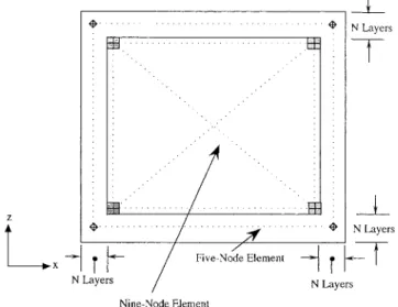
year. The temporal and spatial increments used for computa-tion are⌬t = 0.002 year, ⌬x = 0.02 km, and ⌬z = 0.02 km for both nine-node and five-node elements. This condition refers to a transient transport problem with a maximal Peclet number of one. It is useful to investigate numerical accuracy when the five-node elements are involved. The nine-node elements are placed in the interior domain, and N-row and N-column five-node elements are positioned at boundaries, as shown in Fig. 5. The element layout is essentially designed for assessing ac-curacy of the five-node elements in a domain with irregular boundaries. There are four different N values used in the nu-merical experiments, i.e., N = 0, 2, 5, and 10. The simulated results are shown in Fig. 6. For N = 0, only the nine-node elements are used for numerical simulation. The simulated contours of the solute concentration are plotted in solid line, as presented in Fig. 6(a). The contours agree very well with those of the analytical solution plotted in a dashed line. Fig. 6(b) refers to N = 2, and no visible difference is found as compared with the numerical solution of N = 0. The numerical solution of N = 5 is presented in Fig. 6(c), the contours of which are slightly different from the numerical solutions of N = 0 and 2. When N is increased to 10, the simulated contours of solute concentration, as shown in Fig. 6(d), deviate signif-icantly from those of the analytic solution. The average nodal errors described by the solute concentration compared with the analytical solutions are 0.0022, 0.0025, 0.0031, and 0.015 for

N = 0, 2, 5, and 10, respectively. The finite analytic method

used here is not an integral method; therefore, the global mass conservation is not guaranteed. Adequate conservation of global mass is a necessary but not a sufficient condition for acceptability of a numerical simulator. Nevertheless, the ratios of global mass conservation associated with Fig. 6 are found in between 99.0 and 99.9%. This indicates that the numerical accuracy is directly related to nodal error but may not be closely related to the global mass conservation in the finite analytic method.

FIG. 4. Numerical Experiments on Nine Weighting Schemes Used to Evaluate Unsaturated Hydraulic Conductivity: (a)⌬z = 1.0 cm;

(b)⌬z = 0.5 cm; (c)⌬z = 0.2 cm (●: Experimental Data; 1: Central Node; 2: Arithmetic Mean; 3: Arithmetic Mean with Extra Central

Weighting; 4: Geometric Mean; 5: Geometric Mean with Extra Central Weighting; 6: Harmonic Mean; 7: Upstream Weighting with Arith-metic Mean; 8: Upstream Weighting with Geometric Mean; 9: Upstream Weighting with Harmonic Mean)

Based on the above findings, we can see that the advantage of using the five-node element is that we may match the ir-regular boundaries while remaining on the Cartesian coordi-nate system. Therefore, the system of algebraic equations can be solved through simple, straightforward, line-by-line itera-tion. The disadvantage is that the accuracy of the five-node element is not as good as that of nine-node element, especially

in the case that the flow advection comes from a direction with an inclined 45⬚ angle to the x or z coordinates. However, for the purpose of matching the irregular boundaries, only very few five-node elements placed at the boundaries are required. In general, only one five-node element is needed. Eventually, it would not deteriorate the overall accuracy. The comparisons noted above indicate that the finite analytic method is capable

FIG. 5. Layout of Computational Grids Using Nine-Node Ele-ments Placed in Interior Domain and Using N Layers of Five-Node Elements Placed at Boundaries for Verification of Solute Transport Problem

FIG. 6. Comparison of Contours of Solute Concentration at Time = 0.4 Years in Verification Problem between Finite Analytic Numer-ical Solution and AnalytNumer-ical Solution Using N Layers of Five-Node Elements Placed at Boundaries of Computational Domain: (a) N = 0; (b) N = 2; (c) N = 5; (d) N = 10

of simulating solute transport problems with spatially variable advection and dispersion coefficients under a presumed con-dition of geometric irregularity by using mixed nine-node and five-node elements. In an unsaturated zone, the nonlinear be-havior of fluid flow and solute transport acts in a similar way to the nonuniform advective and dispersive processes in a sat-urated zone. Therefore, the verification addressed above is transposable for solute transport in an unsaturated zone.

NUMERICAL ASSESSMENT OF SOLUTE MIGRATION FROM LANDFILL IN UNSATURATED ZONE

Problem Description

In the following example, the solute migration along the vertical in unsaturated zone is presented. The ground-water table is situated below the landfill, as sketched in Fig. 7. To protect the natural environment of ground water, it is important to estimate the travel time of the polluted solute from reaching the ground-water table and predict the potential spatial distri-bution of solute concentration in the unsaturated zone. The illustrated example entails a landfill with an irregular ground surface. During the rainfall season, the solute water within the landfill may infiltrate into the unsaturated zone and propagate downward. Finally, the polluted solute may reach the ground-water table and contaminate ground ground-water.

FIG. 7. Schematic Representation of Solute Plume Released from Landfill with Irregular Ground Surface

FIG. 8. Contours of Solute Concentration Obtained from Simulation of Landfill Leaching Using Kd= 0 and␭ ⫺0: (a) Time = 15 Days;

(b) Time = 30 Days

In the present study, the exponential forms of the constitu-tive functions of soil, K(H) and␪(H), are used (Warrick and Lomen 1976). K(H) and␪(H) are given, respectively, as

K(H ) = K exp(o ␤H) (16)

and

␪(H) = (K /A ) exp(␤H)o o (17)

in which Ko and Ao are empirical constants for the soil. Ko =

0.0020 cm/min,␤ = 0.01, and Ao = 0.004 cm/min. These

pa-rameters refer to a low permeability of soil like clay or silt, which can be placed beneath the landfill to reduce the infiltra-tion rate. The bulk density of the clay loam,␳b, is 1.55 g/cm

3

. The dispersivity of soil for solute transport is scale dependent. Transversal dispersivity␣tranges typically from 10 to 40% of

longitudinal dispersivity␣1. For the scale shown in Fig. 7,␣1

= 10 m and␣t= 3 m are reasonable assumptions for the

sat-urated zone (Anderson 1979). Here, we assume it is also ap-plicable for the unsaturated zone.

To predict the fluid flow and solute transport in the unsat-urated zone for a domain with irregular boundaries, as en-closed by the dashed line in Fig. 7, the five-node and nine-node elements are used to form the grid system in the computational domain. During the rainfall season, the water flux leaking from the bottom of the landfill into the unsaturated zone is taken as 0.024 cm/hr. This amount of flux is small due

to the low permeable substance placed on the bottom of the landfill. In addition, the water flux from the sloping ground surface infiltrating into the unsaturated zone is 0.12 cm/hr. The boundary conditions and computational grids used for simu-lation can be found in Tsai et al. (1993).

The initial condition of the pressure head, H, in the unsat-urated zone is assumed⫺100 cm beneath the ground surface and is linearly distributed between the ground surface and the ground-water table. The initial solute concentration is zero everywhere. Variable time increments are used in the compu-tation. Three-hour time intervals are used for the first day, and 24-hour time intervals are used thereafter. For each time level, the solution is obtained by the line-by-line iteration in the z direction from the low to the top boundaries until the differ-ence of H and C* (= C␪) between successive iterations is less than 0.001 cm and 0.00001, respectively. It is a two-step nu-merical procedure. The unsaturated flow equation, (1), is solved first. Then the output, including the flow field and mois-ture contents obtained by solving (1), is taken as an input for solving the solute transport equation, (2).

Results and Discussion

The contours of solute concentration in the unsaturated zone for times equal to 15 and 30 days are shown in Figs. 8(a and b), respectively. These two figures reveal that transversal mi-gration of solute is not so significant as compared with the longitudinal (downward) migration. Besides, the solute con-centration 0.1 is found to reach the ground-water table at 30 days of travel time. Another finding of the numerical solution of unsaturated flow is that the finite analytic coefficients within a local element are all positive and the summation is one. The finite analytic coefficients for the numerical solutions of solute transport are all positive as well. Although the physical decay coefficient, ␭, is zero here, the numerical decay coefficient [␭ ⫹ (1/R)(⭸Vx/⭸x) ⫹ (1/R)(⭸Vz/⭸z)], s seen in Table 1, is a

nonzero term. Therefore, the summation of the finite analytic coefficients in an element is found to be less than, but close to, one. The maximal Peclet numbers in the simulation of un-saturated flow and solute transport are found to be about 0.6 and 1.2, respectively, Magnitude of the Peclet number near this range is close to the standard suggested by Leonard and Mokhtari (1990) for consideration of satisfactory numerical accuracy.

From the simulation and results of the landfill applications, we found some advantages of the numerical model. Since the finite analytic method is an analytically based method, the truncation error can be minimized, and the numerical stability

is robust. Because the advection-diffusion equation is the basic form for deriving the finite analytic numerical solution and the flow and transport equations in the unsaturated zone are both the advection-diffusion partial differential equations, only one formulation is required but applied to both. This feature en-hances the numerical efficiency. Moreover, the current numer-ical model is shown to be able to simulate practnumer-ical problems like solute transport under a landfill in an unsaturated zone with an irregular ground surface by proper use of mixed five-node and nine-five-node elements. Since the structured-grid system is used, the layout of the grid is straightforward and the simple line-by-line iteration can be used for convergence process.

Some minor numerical disadvantages may still exist in the above applications. First, the accuracy of the five-node ele-ment and the upwinding effect among nodes are worse than those of the nine-node element. Fortunately, only one five-node element is required to place at the irregular boundaries. Secondly, the use of five-node and nine-node elements in a structured-grid system may increase the total number of com-putational nodes and, hence, the computing time. Finally, the adaptive grid associated with the refinement of the local grid may be not easily accessible to the proposed structure-grid system, and further development is required.

CONCLUDING REMARKS AND SUGGESTIONS

The purpose of the present study is to invoke the finite an-alytic method to solve the vertical, two-dimensional subsurface flow and transport equations in the unsaturated zone. In the finite analytic method, the coefficients of the governing equa-tions are frozen in each element, so that linear partial differ-ential equations can be obtained and solved. A spatial weight-ing scheme is used to evaluate the averaged unsaturated hydraulic conductivity in the discretized element. The geo-metric mean schemes, among the nine potential spatial weight-ing schemes, are found to better capture the sharp wettweight-ing front of the infiltration data. In solving the subsurface transport problem, this study illustrates how to use mixed five-node and nine-node elements to match a domain with irregular bound-aries and achieve the required numerical accuracy. The appli-cations of the developed numerical model to the landfill dem-onstrate that the finite analytic numerical solutions for subsurface flow and transport in the unsaturated zone preserve the nature of mass decay, result in a matrix of the positive type, increase the mesh Peclet number of stability, and feature an unconditionally stable scheme. Moreover, the use of the structured-grid system enables the line-by-line iteration to be readily applicable in solving the matrix of the system of the algebraic equation. However, the disadvantage associated with an adaptive grid may arise when dealing with the local refine-ment of the grids. Furthermore, to achieve the optimal nu-merical performance, an effective grid generation algorithm enabling proper use of the five-node and nine-node elements to automatically match irregular boundaries of the computa-tional domain would be very useful.

ACKNOWLEDGMENTS

The study was funded by the National Science Council, Taiwan under Grant No. NSC-86-2211-E-321-001.

APPENDIX I. REFERENCES

Anderson, M. P. (1979). ‘‘Using models to simulate the movement of contaminants through groundwater systems.’’ Critical Rev. in Envir. Control, 9(2), 97–156.

Bear, J. (1979). Hydraulics of groundwater water. McGraw-Hill, New York, 213–234.

Carslaw, H. S., and Jaeger, J. C. (1971). Conduction of heat in solids. Oxford University Press, London.

Carlson, K. D. (1993). ‘‘Finite analytic numerical simulation of

two-dimensional flow problems with irregular boundaries in Cartesian co-ordinates,’’ MS thesis, Dept. of Mech. Engrg., University of Iowa, Iowa City, Iowa.

Chen, C. J. (1989). ‘‘Finite analytic numerical method.’’ Handbook of numerical heat transfer, Wiley, New York.

Chen, C. J., and Chen, H. C. (1984a). ‘‘Development of finite analytic numerical method for unsteady two-dimensional Navier-Stokes equa-tion.’’ J. Comp. Physics, 53(2), 209–226.

Chen, H. C., and Chen, C. J. (1984b). ‘‘Development of finite analytic numerical method for unsteady three-dimensional Navier-Stokes equa-tions: computation of internal flows.’’ ASME FED, 14, 159–165. Haverkamp, R., and Vauclin, M. (1979). ‘‘A note on estimating finite

difference interblock hydraulic conductivity values for transient unsat-urated flow problems.’’ Water Resour. Res., 15(1), 1354–1360. Hwang, J. C., Chen, C. J., Sheikhoslami, M., and Panigrahi, B. K. (1985).

‘‘Finite analytic numerical solution for two-dimensional groundwater solute transport.’’ Water Resour. Res., 21(90), 1354–1360.

Leonard, B. P., and Mokhtari, S. (1990). ‘‘Beyond first-order upwinding: the ultra-sharp alternative for non-oscillatory steady-state simulation of convection.’’ Int. J. Numer. Methods in Engrg., 30, 729–766. Li, W., Xie, Q., and Chen, C. J. (1989). ‘‘Finite analytic solution of flow

over spillways.’’ J. Engrg. Mech., ASCE, 115(12), 2635–2647. Pi, Z., and Hjelmfelt Jr., A. T. (1994). ‘‘Hybrid finite analytic solution of

lateral subsurface flow.’’ Water Resour. Res., 30(5), 1471–1478. Tien, H. C. (1992). ‘‘Finite analytic method for computational domain

with irregular boundaries,’’ PhD thesis, Dept. of Appl. Math., Univer-sity of Iowa, Iowa City, Iowa.

Touma, J., and Vauclin, M. (1986). ‘‘Experimental and numerical analysis of two phase infiltration in a partially saturated soil.’’ Transport in Porous Media, 1, 28–55.

Tsai, W. F., Chen, C. J., and Tien, H. C. (1993). ‘‘Finite analytic numerical solutions for unsaturated flow with irregular boundaries.’’ J. Hydr. Engrg., ASCE, 119(11), 1274–1298.

Warrick, A. W., and Lomen, D. O. (1976). ‘‘Time-dependent linearized infiltration. III: Strip and disc sources.’’ Soil Sci. Soc. Am. J., 40, 639– 643.

Yeh, G. T. (1987). ‘‘FEMWATER: a finite-element model of water flow through saturated-unsaturated porous media.’’ Rep. ORNL-5567/R1, Oak Ridge National Laboratory, Oak Ridge, Tenn.

Yeh, G. T., and Ward, D. S. (1980). ‘‘FEMWATER: a finite-element model of water flow through saturated-unsaturated porous media.’’ Rep. ORNL-5567, Oak Ridge National Laboratory, Oak Ridge, Tenn. Zeng, X. J., and Li, W. (1987). ‘‘The stability and convergence of finite

analytic method for unsteady two-dimensional convective transport equations.’’ Turbulence measurements and flow modeling, C. J. Chen, L. D. Chen, and F. M. Holly, eds., Hemisphere Publishing, Bristol, Pa., 427–433.

APPENDIX II. NOTATION

The following symbols are used in this paper:

A = x-direction locally linearized advective coefficient in

ba-sic form of finite analytic equation;

B = z-direction locally linearized coefficient in basic form of

finite analytic equation;

bi = finite analytic coefficients of five-node solution algebraic

equation;

C = solute concentration; CS = specific moisture capacity;

C* = C␪;

ci = finite analytic coefficients of nine-node solution

alge-braic equation;

G = z-direction diffusion parameter shown in basic form of

finite analytic equation;

g = source function in locally linearized governing equation; H = pressure head;

h = horizontal grid spacing used in element; K = hydraulic conductivity;

Kd = distribution coefficient;

k = vertical grid spacing used in element; n = nth time step;

P = central node in rectangular local element; R = retardation factor;

T1/2 = half-life time of mass decay; t = time;

x, z = spatial coordinates;

x⬘, z⬘ = 45⬚ rotational spatial coordinates; z* = transformed coordinate of z coordinate; ␣l = longitudinal dispersivity;

␣t = transversal dispersivity;

⌬t = time interval;

⌬x = grid spacings used in x direction; ⌬z = grid spacings used in z direction;

␪ = volumetric water content; ␭ = first-order decay coefficient;

⌽ = dependent variable of finite analytic solution; and ␻ = time-weighting factor.