A Deployment Strategy for Mobility-Assisted Wireless Sensor Networks

A Deployment Strategy for Mobility-Assisted Wireless Sensor Networks

Tian-Wen Song

,

Chao-Yang Lee

, Fwu-Tian Lin

,

and Chu-Sing Yang

1

Department of Computer Science and Engineering, National Sun Yat-Sen University

2

Department of Applied Internet Science, Hsing Kuo University

3

Department of Electrical Engineering, National Cheng Kung University

[email protected]

Abstract

Keywords: Deployment, Hybrid Wireless Sensor Network, Hexagonal Virtual Grid, Coverage.

1. Introduction

In a wireless sensor network (WSN), the sensor coverage in the field is always the fundamental requirement for the applications of environmental monitoring. And, sensor deployment becomes the important issue since coverage correlates closely with the deployment [1]. The early proposed works for sensor deployment [2, 3, 4, 5] assumed sensors are all static. In many conditions, manual sensor deployment is not practical. Instead, a random deployment such as sprinkling sensors from the air becomes applicable. However, it often causes both uneven sensor distribution and insufficient field coverage. Many later related works [6, 7, 8, 9, 10] assumed sensors are mobile, and coverage ratio of sensing field can be increased by the sensor movements. For balancing the trade-off between sensor cost and coverage, both static and mobile sensors could be employed in a WSN [11, 12]. This paper proposes a grid-based sensor deployment strategy to improve the sensor coverage for the mobility-assisted WSN, that is, a hybrid WSN which consists of both static and mobile sensors.

2. Background and Assumptions

A sensor device in the WSN may have location finding system and mobilizer as its additional components besides the basic components of processor, memory, micro sensor, RF transceiver, and power [13]. Regarding the location finding system for a WSN, many related researches [14, 15, 16, 17, 18] of the sensor positioning and localization techniques were proposed. By this reason, we assume that the sensors utilized in our works can obtain their location and send the coordinates information to the sink node for further processing. Additionally, due to the related works of sensor devices with mobility techniques had been proposed in [19, 20], we also assume that mobile sensors in the network can move freely, this is not unrealistic in the real world. The other assumptions in this work are that each sensor has the same sensing radius; sensors will be randomly deployed to the sensing field at the initial phase; each sensor will sent location information to the network coordinator (sink node); and, proposed algorithms run as a centralized approach.

3. Proposed Deployment Strategy

3.1. Hexagonal Virtual Grid

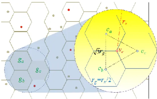
Once all sensors have been randomly deployed in the sensing field, the field will be divided into hexagonal virtual grids upon the cellular concept in telecommunication systems that hexagonal cells have the largest coverage area and smallest overlap compared with square and equilateral triangle ones according to their original coverage circles. In this paper, we define the grid radius rg as

2 / s

g r

r  (1) , where rs is the sensing radius of a sensor. This

definition implies that first, any sensor located within a grid will fully cover the grid, and second, once a sensor is located at the common vertex of three pairwise neighbored grids, it will fully cover

the three grids (Shown as Fig. 1). Accordingly, sensors located in the same grid have same coverage contributions to that grid and they may have no need to be all active at the same time for the purpose of saving energy and extending network lifetime, although this will bring a little reduction of coverage contribution to the other grids (details will be described later). On the other hand, for the purpose of increasing coverage contribution, each mobile sensor is expected to move to a common vertex of three pairwise neighbored grids which need to be covered. The preliminary assumption in this paper is that the sensing field is divided into ng virtual grids

denoted as grid set G={gi | i=1, 2, 3, ..., ng}, and

V={vi | i=1, 2, 3, …, nv} is the set of all nv vertexes

in the field. It is satisfied that g c c b c a c c d v c d v c r v d( , ) ( , ) ( , ) (2) g g a c c b b a c d c c d c c r r c d 3 6 cos 2 ) , ( ) , ( ) , (      (3)

, where ca, cb, and cc are the center points of the

three pairwise neighbored grids ga, gb, and gc. And

vc is their common vertex.

Figure 1. Virtual grids in the sensing field

3.2. Basic Grid-based Deployment

Due to the uneven sensor distribution and insufficient field coverage caused by initial random deployment, some areas, called coverage holes, are not covered by any sensor device, that is, events occur in these holes will not be detected. Therefore, sizes and positions of the coverage holes should be calculated and healed to achieve the coverage requirement. Since a grid will be one hundred percent fully covered if at least one sensor was located in it, our first basic algorithm defines the hole size of grid gi, denoted as Hi, is

g n i1,2,3,...,       otherwise , 1 1 ) ( if , 0 _{s i} i g N H (4)

, where Ns(gi) denotes the number of static sensors

within the grid gi. By reason of that mobile sensors

would have movements, only static sensors are considered in the function Ns. Besides, since a

static sensor could be exactly located at the common edge of two grids or at the common vertex of three grids, it is possible that



, where ns is the total number of static sensors in

the sensing field. Base on the formula (4), We define Gvi as the grid set of three pairwise

neighbored grids with the common vertex vi, and

define Hvi as the total hole size of these grids or the

hole size of vertex vi.

v n i1,2,3,...,  } ] , 1 [ , ) , ( | { j j i g g v g d c v r j n G_i    (6)



, where |Gvi|=3, and 0  Hvi  3. After calculating

the hole size of each vertex, the vertex with largest hole should be healed firstly by dispatching a mobile sensor to cover it. Assume vertex v has the largest hole, and v is shared by the grids ga, gb, and

gc with center point ca=(xa, ya), cb=(xb, yb), and

cc=(xc, yc) respectively. i i v i i V v H v f v f v   ( ), where ( ) max arg (8) ) 3 , 3 ( ) , ( v v a b c a b c y y y x x x y x      (9)

, where (xv, yv) is the coordinates of vertex v, and

also the target position a selected mobile sensor will move to. After the healing, the vertex with second largest hole according to previous calculation cannot be the next healing target because of previous healing could contribute coverage for the nearby grids, that is, the hole sizes of some grids and vertexes may change. An illustration shown in Fig. 2(a) indicates that

H1=H2=H3=H5=1, H4=H6=0, and the grids g1, g2,

g3, and g5 need to be coverd by the healing process.

Gv1={g1, g2, g3}, Gv2={g2, g3, g4}, Gv3={g4, g5, g6};

and Hv1=3; Hv2=2; Hv3=1; Due to the hole size

Hv1>Hv2>Hv3, v1 should be firstly healed. Notice

that once a mobile sensor was selected to heal the hole of v1, the sensor will contribute the full

and Hv3=1. So, the next healing target should be v3,

not v2. By this reason, a recalculation of hole sizes

should be made after each coverage hole healing.

(a) (b) Figure 2. An illustration of healing the hole As shown in Fig. 3, according to the influence of coverage contribution brought by previous hole healing, only the vertexes which is at a distance of less than 2rg from the previous healed one may

need to recalculate their hole sizes. Additionally, the vertexes which have a zero hole size have no need to recalculate. Let vh be previous healed

vertex and V’ be the set of vertexes need a recalculation, then } ] , 1 [ , 0 and 2 ) , ( { ' v_i dv_i v_h r_g H_v i n_v V i    (10)

Figure 3. Vertexes may need to recalculate hole

3.3. Extended Grid-based Deployment

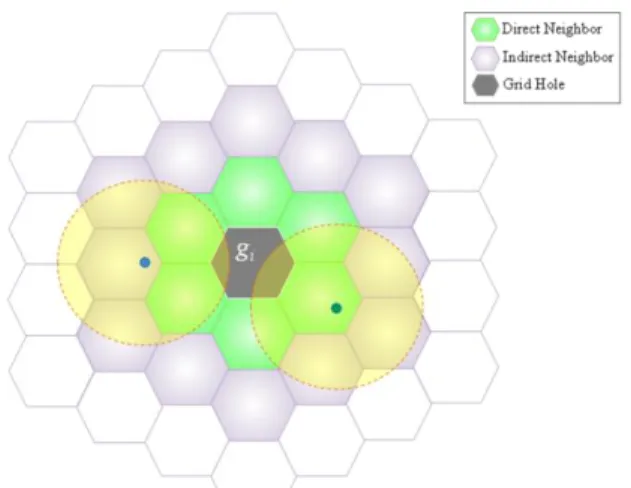
In this section we describe our second algorithm which improves the basic algorithm described above. In the basic algorithm, a grid with no sensor in it was treated as one hole. It can be precisely improved to calculate the hole size for a grid, and further, a precise vertex hole size will be obtained for achieving a higher effect of healing process. Fig. 4 shows that a grid has the possibility of being partially covered by the static sensors within its direct and indirect grid neighbors.

Figure 4. Partially covered by nearby sensors Accordingly, we redefined the hole size, Hi, of

grid gi as following g n i1,2,3,...,                              i i s B s i i i s B s i i i s R s i i i S g C Area g Area S g C g Area g g C B R S H i i )), ( ( ) ( and ) ( ), ( ) ( that set a or , 0    (11)

, where Si denotes the set of static sensors in grid gi;

Bi, the set of static sensors in direct and indirect

neighbor grids of gi; Cs, the region covered by

sensor s; and Area() is the function of area size. The obtained value of Hi indicates the precise real

size of the hole region in the grid gi.

The calculation of vertex hole size Hvi of the

extended grid-based deployment is same as the formulas (6) and (7) shown in section 3.2, but it will get a precise result for hole healing process since the hole calculation of individual grid is more precise than the one in formula (4). Once a mobile sensor was selected to heal the hole of a vertex vi, the sensor will contribute the full

coverage to the all grids in Gvi and partial coverage

to some of the others not belong to Gvi. Therefore,

some vertexes may need a hole size recalculation for next vertex selection of healing process. Also, vertexes with a zero hole size have no need to do so. Fig. 5 shows the possible vertexes need to recalculate hole zise, and formula (12) indicates the necessary vertexes, denotes as V’, need to recalculate. It is a little different from the one described in section 3.2. } ] , 1 [ , 0 and 4 ) , ( { ' v_i d v_i v_h r_g H_v i n_v V i     (12)

Figure 5. Vertexes may need to recalculate hole

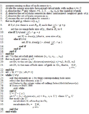
Figure 6. Extended grid-based algorithm

3.4. Mobile Sensor Selection

The mobile sensors in the sensing field will be selected to heal the holes one by one. Each time the vertex with largest hole will be chosen as the moving target for a mobile sensor. Regarding the mobile sensor selection, since the shorter moving distance will save more energy for the sensor, our first rule is that the sensor which is closest to the target vertex will be chosen firstly.

) , ( ) , ( }, { ' such that ' select h i h a a i a v m d v m d m M M m M M m        (13)

, where M denotes the set of all mobile sensors; M’ is the set of previous selected sensors; and vh is the

target vertex.

However, the selection strategy can be improved

by the second rule for the cases in following Fig. 7. The hole of vx is larger than the one of vy, and the

green line is the path result determined by rule-1. The rule-2 will make an exchange of targets, if

) , ( ) , ( ) , ( ) , (ma vx d mb vy d mb vx d ma vy d    (14)

, where the average moving distance of sensors will be reduced further. Notice that actual movements of all the mobile sensors will happen after all dispatch selection are finished since the algorithms are centralized.

(a) (b)

Figure 7. Examples of moving target exchange

Figure 8. Mobile sensor dispatching algorithm

3.5. Redundant Sensors

Regarding the situation shown in the Fig. 9(a), all the sensors in the same grid contribute full coverage of that grid and they have a great overlap in coverage. Accordingly, besides the reserved one, the others can be treated as the redundant sensors which can be scheduled into sleep mode and be waked up as active sensors on demand. Similarly, Fig. 9(b) shows the mobile sensor will contribute full coverage to the three pairwise neighbored grids with the common vertex healed. Therefore,

all the static sensors in these three grids can be treated as redundant sensors, too. Scheduling the redundant sensors into sleep mode will make a little reduction of coverage, nevertheless, they can help to extend the lifetime of the sensor network. This is a tradeoff situation. The influence of redundant sensors on coverage will be shown in the next section which describes the results of network simulation.

(a) (b) Figure 9. Redundant sensors

4. Performance Evaluation

The performance was evaluated by network simulation of proposed algorithms. BGD means basic grid-based deployment while EGD means extended one. Furthermore, BGD-A and EGD-A represent all sensors are active while BGD-S and EGD-S represent redundant sensors are in sleep. The environment parameters of simulation are as

Sensing field: 490m x 360m Sensing radius: 40m Grid radius: 20m

Number of sensors: 60/80/100 (three cases) Mobile sensors: 0% ~ 50% (10% Interval) Simulation runs: each case has 150 runs

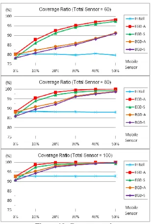
Fig. 10 shows the curves of coverage ratio of 60, 80, and 100 total sensors with 0%~50% mobile sensors. The cyan curve in each figure indicates the initial coverage, and naturally, the more sensors bring the higher ratio. The BGD and EGD algorithms have the significant improvements of the coverage ratio, especially the EGD algorithms obtained higher ratio than the BGD ones because of precise calculation of coverage holes. The evaluation results also show the EGD-S and BGD-S has a little decrease than EGD-A and BGD-A respectively. The decreases are caused by the slept redundant static sensors due to the lack of their coverage contribution. The coverage ratio is even a little less than the initial one where 0% mobile sensor was employed. Nevertheless, the redundant sensors have the contribution to extend the network lifetime. We can see the trade-off between the coverage and the number of redundant sensors from the views of Fig. 10 and Fig. 12.

Figure 10. Coverage ratio

In Fig. 11, it shows that the strategy of mobile sensor selection for healing coverage holes can help decrease the average moving distance of selected mobile sensors by performing selection rule 1&2 described in section 3.4. And therefore, it can aid the power saving for the sensors.

Figure 11. Average moving distance

Fig. 12 shows the number of redundant static sensors appear in EGD-S deployment algorithm. Although a little coverage will be influenced, these sensors can help to extend the network lifetime by utilizing active/sleep scheduling. Since the increase of mobile sensors leads to the decrease in static sensors, the curve has a downward tendency. And naturally, more sensors in the sensing field will bring more redundant sensors due to the density.

5. Conclusion

This paper utilized hexagonal virtual grids and proposed the grid-based sensor deployment algorithms for the hybrid wireless sensor networks, which consist of both static and mobile sensors. It makes the improvements of coverage ratio, considers the reduction of sensor moving distance, and introduces the influence of redundant sensors. Evaluation shows proposed deployment strategy obtained the significant effect of performance.

References

[1] S.K. Meguerdichian, F. Potkonjak, M. Srivastava, and M.B. Srivastava, “Coverage Problems in Wireless Ad-hoc Sensor Networks”, Proc. IEEE

INFOCOM 2001, Anchorage (Alaska), USA, pp.

1380-1387, April 22-26, 2001.

[2] T. Clouqueur, V. Phipatanasuphorn, P. Ramanathan, and K.K. Saluja, “Sensor Deployment Strategy for Target Detection”, Proc. 1st ACM International

Workshop on Wireless Sensor Networks and Applications, Atlanta (Georgia), USA, pp. 42-48,

September 28, 2002.

[3] S.S. Dhillon, K. Chakrabarty, and S.S. Iyengar, “Sensor Placement for Grid Coverage under Imprecise Detections”, Proc. 5th International

Conference on Information Fusion, Annapolis

(Maryland), USA, pp. 1581-1587, July 8-11, 2002. [4] S. Kumar, T.H. Lai, and J. Balogh, “On k-coverage

in a mostly sleeping sensor network”, Proc. 10th

ACM Annual International Conference on Mobile Computing and Networking, Philadelphia (Pennsylvania), USA, pp. 144-158, September 26-October 1, 2004.

[5] O. Rahman, A. Razzaque, and C.S. Hong, “Probabilistic Sensor Deployment in Wireless Sensor Network: A New Approach”, Proc. 9th

International Conference on Advanced Communication Technology, Phoenix Park, South

Korea, pp. 1419-1422, February 12-14, 2007. [6] G. Wang, G. Cao, T.L. Porta, and W. Zhang,

“Sensor Relocation in Mobile Sensor Networks”,

Proc. IEEE INFOCOM 2005, Miami (Florida),

USA, pp. 2302-2312, March 13-17, 2005. [7] S. Chellappan, X. Bai, B. Ma, and D. Xuan,

“Sensor Networks Deployment Using Flip-Based Sensors”, Proc. 2nd IEEE International Conference on Mobile Ad-hoc and Sensor Systems,

Washington (DC), USA, pp. 291-298, November 7-10, 2005.

[8] G. Wang, G. Cao, and T.L. Porta, “Movement-assisted sensor deployment”, IEEE

Transactions on Mobile Computing, vol. 5, no. 6,

pp. 640-652, June, 2006.

[9] S. Yang, M. Li, and J. Wu, “Scan-Based Movement-Assisted Sensor Deployment Methods in Wireless Sensor Networks”, IEEE Transactions

on Parallel and Distributed Systems, vol. 18, no. 8,

pp. 1108-1121, August, 2007.

[10] X. Wu, J. Cho, B.J. D'auriol, and S. Lee, “Mobility-Assisted Relocation for Self-Deployment in Wireless Sensor Networks”,

IEICE Transactions on Communications, vol.

E90-B, no. 8, pp. 2056-2069, August, 2007. [11] G. Wang, G. Cao, P. Berman, and T.L. Porta,

“Bidding Protocols for Deploying Mobile Sensors”, IEEE Transactions on Mobile Computing, vol. 6, no. 5, pp. 515-528, May, 2007.

[12] X. Wu, J. Cho, B.J. d'Auriol, S. Lee, and H.Y. Youn, “Self-deployment of Mobile Nodes in Hybrid Sensor Networks by AHP”, Lecture Notes

in Computer Science, 4611, pp. 663-672, 2007.

[13] K. Sohraby, D. Minoli, and T. Znati, Wireless

Sensor Networks: Technology, Protocols, and Applications, Wiley, Hoboken, 2007.

[14] S. Capkun, M. Hamdi, and J.P. Hubaux, “GPS-free positioning in mobile Ad-Hoc networks”, Hawaii

International Conference on System Sciences,

HICSS-34, Wailua (Hawaii), USA, January 3-6, 2001.

[15] N. Bulusu, J. Heidemann, and D. Estrin, “GPS-less Low Cost Outdoor Localization For Very Small Devices”, IEEE Personal Communications, vol. 7, no. 5, pp. 28-34, October,

2000.

[16] D. Niculescu and B. Nath, “Ad Hoc Positioning Systems (APS) Using AoA”, Proc. IEEE

INFOCOM 2003, San Francisco (California), USA,

pp. 1734- 1743, March 30-April 3, 2003.

[17] N. Patwari and A.O. Hero III, “Using Proximity and Quantized RSS for Sensor Location in Wireless Location in Wireless Networks”, Proc.

2nd ACM International Conference on Wireless Sensor Networks and Applications, San Diego

(California), USA, pp. 20-29, September 19, 2003. [18] A. Savvides, C. Han, and M.B. Strivastava,

“Dynamic Fine-Grained Localization in Ad-Hoc Networks of Sensors”, Proc. ACM MOBICOM

2001, Rome, Italy, pp. 166-179, July 16-21, 2001.

[19] G.T. Sibley, M.H. Rahimi, and G.S. Sukhatme, “Robomote: A Tiny Mobile Robot Platform for Large-scale Sensor Networks”, Proc. IEEE

International Conference on Robotics and Automation, Washington (DC), pp. 1143-1148,

May 11-15, 2002.

[20] F. Mondada, E. Franzi, and P. Ienne, “Mobile robot miniaturisation: a tool for investigation in control algorithms”, Proc. 3rd International

Symposium on Experimental Robotics, Kyoto,