基於SLA之雲端資料中心負載平衡機制

國

立

交

通

大

學

網路工程研究所

碩

士

論

文

基 於 S L A 之 雲 端 資 料 中 心 負 載 平 衡 機 制

An SLA-aware Load Balancing Scheme for

Cloud Datacenters

研 究 生：黎中誠

指導教授：王國禎 教授

基於 SLA 之雲端資料中心負載平衡機制

An SLA-aware load balancing scheme for cloud datacenters

研 究 生：黎中誠 Student：Chung-Cheng Li

指導教授：王國禎 Advisor：Kuo-Chen Wang

國 立 交 通 大 學

網 路 工 程 研 究 所

碩 士 論 文

Submitted to Institute of Network Engineering College of Computer Science

National Chiao Tung University in Partial Fulfillment of the Requirements

for the Degree of Master

in

Computer Science June 2012

Hsinchu, Taiwan, Republic of China

i

基於SLA之雲端資料中心負載平衡機制

學生：黎中誠 指導教授：王國禎 博士

國立交通大學網路工程研究所

摘 要

雲端計算這個名詞出現在 2007 年的第四季，它具有高度的可延

展性和接近無限的 (如計算) 資源。如何讓擁有成千上萬的虛擬機器

的大型資料中心達到負載平衡是雲端計算的重要議題之一。在本篇文

章中，我們提出了一種新的非集中式負載平衡結構，稱為雙層非集中

式負載平衡器 (

tldlb

)。這種非集中式負載平衡器擁有可延展性和

高可用性的優點，有利於服務更多雲端使用者。除此之外，我們也提

出一個稱為基於類神經網路之動態加權循環 (

nn-dwrr

) 的動態負載

平衡演算法，它能有效地將大量的使用者請求分配到各個實際提供服

務的虛擬機器上。在

nn-dwrr

演算法中，我們將監控虛擬機器所得的

負載指標(CPU、記憶體、網路頻寬、硬碟存取等四項利用率)和類神

ii

經網路結合，以調整每台虛擬機器的服務權重。我們的

nn-dwrr

演算

法可以利用類神經的預測和最佳化能力，有效減低服務水準協議

(SLA) 的 違 反 率 。 實 驗 結 果 證 明 我 們 所 提 出 的 負 載 平 衡 演 算 法

(

nn-dwrr

) 在資源有限的情況下，其平均回應時間上比

wrr

快 1.86

倍，比 capacity based 快 1.49 倍，以及比 ANN-based 快 1.21 倍。

我們的方法，在相同時間內能處理更多的使用者要求，而與其他負載

平衡演算法相比，更適用於大型雲端資料中心。此外，

tldlb

演算法

可以適時啟動虛擬機器池中的虛擬機器來避免違反 SLA。

關鍵詞：類神經網路、雲端計算、非集中式架構、負載平衡、服務水

準協議。

iii

An SLA-aware Load Balancing Scheme

for Cloud Datacenters

Student: Chung-Cheng Li Advisor: Dr. Kuochen Wang

Department of Computer Science National Chiao Tung University

Abstract

Cloud computing appears at the fourth season, 2007. It has high scalability and nearly unlimited (e.g., computing) resources. One of the most important issues about cloud computing is how to achieve load balancing among thousands of virtual machines (VMs) in a large datacenter. In this paper, we propose a novel decentralized load balancing architecture, called tldlb (two-level decentralized load balancer). This distributed load balancer takes advantage of the decentralized architecture for providing scalability and high availability capabilities to service more cloud users. We also propose a neural network-based dynamic load balancing algorithm, called nn-dwrr (neural network-based dynamic weighted round-robin), to dispatch a large number of client requests to different VMs, which are actually providing services. In nn-dwrr, we combine of VM load metrics monitoring (CPU, memory, network bandwidth, disk I/O utilization) and neural network to adjust the weight of each VM. Our nn-dwrr algorithm can reduce SLA (service-level agreement) violations. Experimental results support that our proposed load balancing algorithm, nn-dwrr, can be applied to a large cloud datacenter, and it is 1.86 times faster than wrr, 1.49

iv

times faster than capacity-based, and 1.21 times faster than ANN-based load balancing algorithms in terms of average response time in the limited resources. In addition, tldlb can avoid SLA violations via in-time activating VMs in the spare VM pool.

Keywords: Artificial neural network, cloud computing, decentralized architecture, load balancing, service level agreement.

v

Acknowledgements

Many people have helped me with this thesis. I deeply appreciate my thesis advisor, Dr. Kuochen Wang, for his intensive advice and guidance. I would like to thank all the members of the Mobile Computing and Broadband Networking Laboratory (MBL) for their invaluable assistance and suggestions. The support by the National Science Council under Grant NSC101-2219-E-009-001 and by the Inventec under Contract 100C202 is grateful acknowledged. Finally, I thank my family for their endless love and support.

vi

Contents

Abstract (in Chinese)……….………...i

Abstract ... iii

Contents ... vi

List of Figures ... vii

List of Tables ... viii

Chapter 1 Introduction ... 1

Chapter 2 Related Work ... 4

2.1 Load balancer architecture ... 4

2.1.1 Centralized architecture ... 4

2.1.2 Decentralized architecture ... 5

2.2 Load balancing algorithms ... 7

Chapter 3 Proposed SLA-aware Load Balancing Scheme for Cloud Datacenters 9 3.1 Two-level decentralized load balancer (tldlb) ... 9

3.2 Neural network-based dynamic weighted round-robin (nn-dwrr) scheduling ... 13

Chapter 4 Evaluation and Discussion ... 18

4.1 Experimental environment ... 18

4.2 Comparison of different load balancing algorithms ... 19

4.3 Comparison of SLA violation rates with and without a spare VM pool ... 23

Chapter 5 Conclusion ... 24

5.1 Concluding remarks ... 24

5.2 Future work ... 24

vii

List of Figures

Figure 1. The cloud scales: Amazon EC2 growth [2]. ... 1

Figure 2. A classic load balancer architecture in a cloud computing environment. ... 2

Figure 3. Three-level centralized load balancer architecture [9]. ... 5

Figure 4. Structure of a decentralized load balancer [8]. ... 6

Figure 5. Structure of a Meta-Scheduler [8]. ... 6

Figure 6. Proposed two-level decentralized load balancer (tldlb) architecture. ... 10

Figure 7. The configuration of an SLA-aware local load balancer along with a spare VM pool. ... 12

Figure 8 Schematic representation of an artificial neural network model for VMi. .... 14

Figure 9. The process of delta learning rule VMi. ... 14

Figure 10. Flowchart of the nn-dwrr algorithm. ... 17

Figure 11. Experimental setup. ... 18

Figure 12. Comparison of four scheduling algorithms (maximum response time specified in the SLA: 2000 ms). ... 20

Figure 13. Average response time (maximum response time specified in the SLA: 2000 ms)... 20

Figure 14. Comparison of four scheduling algorithms (maximum response time specified in the SLA: 1000 ms). ... 21

Figure 15. Comparison of four scheduling algorithms (maximum response time specified in the SLA: 432 ms). ... 21

viii

List of Tables

Table 1. Qualitative comparison of different load balancing architectures. ... 7

Table 2. Qualitative comparison of different load balancing algorithms. ... 8

Table 3. Load balancing experimental parameters. ... 19

Table 4. Configuration of each VM. ... 19

1

Chapter 1

Introduction

Cloud computing is the delivery of computing as a service rather than a product, whereby shared resources, software, and information are provided to computers and other devices as a utility (like the electricity grid) over a network (typically the Internet) [1]. Cloud Computing has been envisioned as the next-generation architecture of IT enterprises. Therefore, it rapidly grows in recent years. We can clearly find that the number of users which use cloud computing grows very fast, as shown in Figure 1.We can see the growth of average daily instance launch counts in Amazon EC2 is very fast.

2

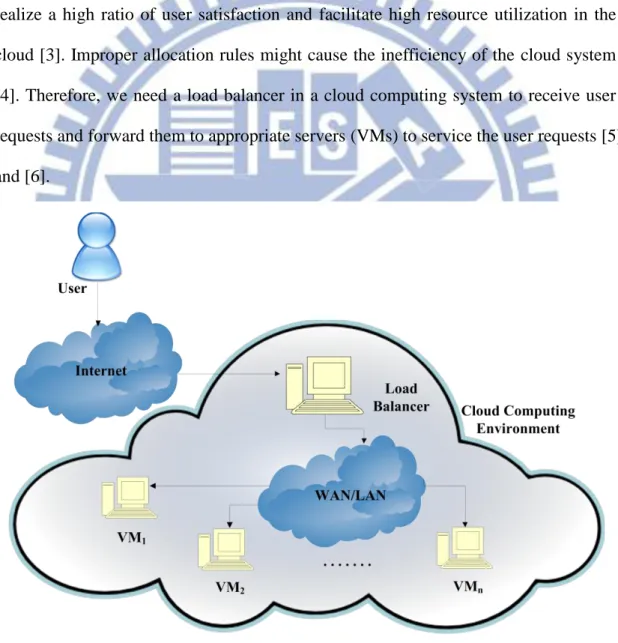
The load of a cloud computing system is highly dynamic. To support a large number of users which use cloud services, cloud service providers must provide shared resources in datacenters located across the world. Different users may require different services, and it may lead to load unbalance between the servers (virtual machines, VMs) in a cloud datacenter. To conquer this problem, user requests are sending to a load balancer and the load balancer then forward them to the appropriate VMs for processing in cloud datacenters. The function of load balancing aims to realize a high ratio of user satisfaction and facilitate high resource utilization in the cloud [3]. Improper allocation rules might cause the inefficiency of the cloud system [4]. Therefore, we need a load balancer in a cloud computing system to receive user requests and forward them to appropriate servers (VMs) to service the user requests [5] and [6].

Figure 2 illustrates a classic load balancer architecture in a cloud computing Figure 2. A classic load balancer architecture in a cloud computing environment.

3

environment. All user requests will be connected to a load balancer. Obviously, we cannot expect one load balancer to maintain the burden of the entire datacenter. We can use a technique which is similar to Amazon’s Auto Scaling. When one load balancer is overloaded, it will start another load balancer to share the load of user requests.

A service-level agreement (SLA) is a part of a service contract where the level of service is formally defined [7]. The SLA will typically have a technical definition in terms of response time, throughput, or similar measurable details [7]. In this paper, we aim to reduce the SLA violation rate while designing a load balancing architecture and algorithm.

In Chapter 2, we describe the architecture and algorithm of a load balancer design in a cloud computing environment and depict the differences between centralized and distributed load balancer designs. Chapter 3 proposes a new architecture, called an SLA-aware two-level decentralized load balancer (tldlb), to support dynamic load balancing in cloud data centers and also proposes a novel load balancing algorithm, called neural network-based dynamic weighted round-robin (nn-dwrr), to dispatch requests to appropriate VMs. Chapter 4 shows experimental results and the comparison of different load balancing algorithms. Finally, Chapter 5 concludes this paper and identifies future work.

4

Chapter 2

Related Work

2.1 Load balancer architecture

There are several load balancing architectures in cloud computing environments [3], [8], [9], [10]. All these architectures, broadly implements load balancing algorithms, which can be static or dynamic, and also uses centralized or decentralized control [8]. Therefore we roughly divide load balancing architectures into two categories, centralized and decentralized. We briefly describe these two architectures as follows.

2.1.1 Centralized architecture

A centralized load balancer architecture has a single load balancer which receives an incoming request and then select a proper VM to serve the request by a scheduling algorithm, as shown in Figure 3. In this architecture, the load balancer may become a bottleneck in cloud environments if the request rate grows to exceed the capacity of the load balancer. That is, this architecture lacks scalability in cloud environments.

5

2.1.2 Decentralized architecture

A decentralized load balancer architecture has several load balancers in cloud environments. Incoming requests will be dispatched to load balancers randomly or adjacent load balancers, as shown in Figure 4. Cluster-1, Cluster-2 and Cluster-3 are composed of resources. Figure 5 shows the configuration of a Meta-Scheduler in Figure 4. Users submit their jobs to a Meta-Scheduler, and the jobs are stored in the queue of a request handler. Dispatch Manager obtains the submitted job periodically from the queue. Load Balancer will perform load balancing by exploiting the information gathered from Load Monitor and Information Manager. Information Manager will query Load Monitor and send the host load information to Load Balancer. Transfer Manager gives permission rights for the execution of a given job to a remote host. Execution Manager will keep updating the job status to Dispatch Manager. Although the decentralized load balancer architecture has more scalability than the centralized load balancer architecture, it needs more communication cost to share load information among load balancers.

6

Figure 4. Structure of a decentralized load balancer [8].

7

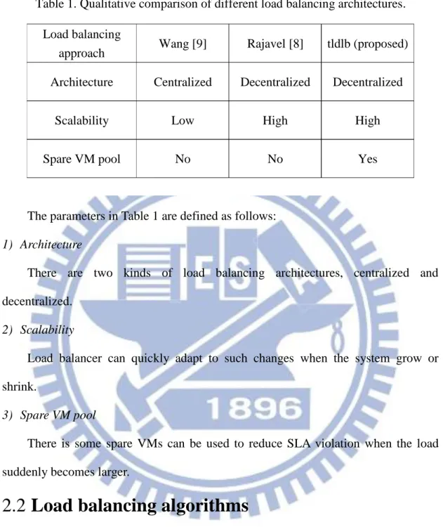
The parameters in Table 1 are defined as follows: 1) Architecture

There are two kinds of load balancing architectures, centralized and decentralized.

2) Scalability

Load balancer can quickly adapt to such changes when the system grow or shrink.

3) Spare VM pool

There is some spare VMs can be used to reduce SLA violation when the load suddenly becomes larger.

2.2 Load balancing algorithms

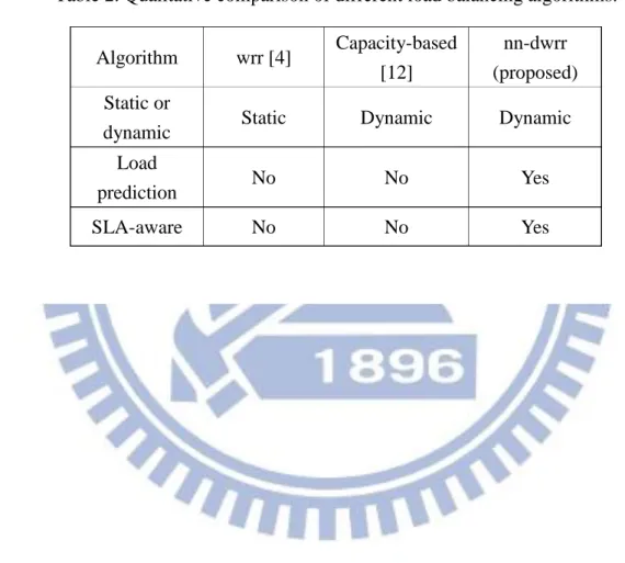
We surveyed two existing load balancing algorithms and proposed a neural network-based dynamic weighted round-robin (nn-dwrr) scheduling algorithm. The first existing scheduling algorithm is called the weighted round-robin scheduling algorithm (wrr) [10]. It assigns a fixed weight to each VM depending on the VM’s processing capacity at the startup. The second capacity-based scheduling algorithm monitors the resources of each VM and distributes more requests to the VM which

Table 1. Qualitative comparison of different load balancing architectures. Load balancing

approach Wang [9] Rajavel [8] tldlb (proposed) Architecture Centralized Decentralized Decentralized

Scalability Low High High Spare VM pool No No Yes

8

has more remaining resources. The main concept is distributing requests to a VM which has the most remaining capacity [12]. The last load balancing algorithm is the proposed neural network-based dynamic weighted round-robin algorithm (nn-dwrr), which adjusts weights based on neural network-based load prediction, and it will be detailed in Chapter 3. Table 2 shows qualitative comparison of different load balancing algorithms.

Table 2. Qualitative comparison of different load balancing algorithms. Algorithm wrr [4] Capacity-based

[12]

nn-dwrr (proposed) Static or

dynamic Static Dynamic Dynamic Load

prediction No No Yes SLA-aware No No Yes

9

Chapter 3

Proposed SLA-aware Load

Balancing Scheme for Cloud

Datacenters

In this paper, we propose an SLA-aware two-level decentralized load balancer (tldlb) architecture and a neural network-based dynamic weighted round-robin scheduling algorithm (nn-dwrr) to support dynamic load balancing in cloud data centers.

3.1 Two-level decentralized load balancer (tldlb)

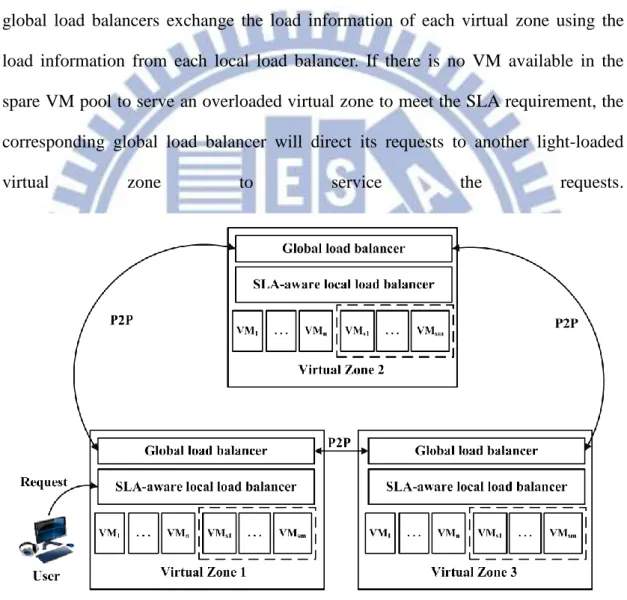
The two-level decentralized load balancer is divided into two levels in our design: global load balancer and local load balancer. Each global load balancer is connected to an SLA-aware local load balancer that forms a virtual zone. The load balancer architecture is shown in Figure 6, which contains two parts, described as follows: 1) Local load balancer

A local load balancer has two main tasks. The first task is monitoring the load of VMs which are in the same virtual zone. The local load balancer will obtain four load metrics (CPU, memory, network bandwidth, disk I/O utilization) from each VM and the response time of each request for VMs. The local load balancer will provide the above information to the global load balancer. If the current working VMs (VM1

through VMn) can’t handle the load, the local load balancer will activate some spare

10

task is choosing an appropriate VM using a neural network-based load balancing algorithm and then redirects the request to the VM. Our local load balancer is SLA-aware, which means we assign user requests to appropriate VMs for service so as to meet SLA requirements.

2) Global load balancer

Global load balancers are connected to each other via P2P connections. The global load balancers exchange the load information of each virtual zone using the load information from each local load balancer. If there is no VM available in the spare VM pool to serve an overloaded virtual zone to meet the SLA requirement, the corresponding global load balancer will direct its requests to another light-loaded virtual zone to service the requests.

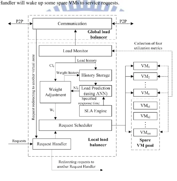
Figure 7 shows the modules inside an SLA-aware local load balancer along with a spare VM pool. The following is a brief description of each module.

 Request Handler

11

This module receives user requests and forwards them to the Request Scheduler module. When the workload of a virtual zone reaches the upper limit, this module will redirect requests to another Request Handler which belongs to another virtual zone.  Request Scheduler

This module assigns requests from Request Handler to selected VMs based on the weights from the Weight Adjustment module. We give each VM a weight and then the Request Scheduler module distributes requests to appropriate VMs by these weights.

 Load Monitor

It monitors four utilization metrics (CPU, memory, network bandwidth, disk I/O utilization) of each VM in this local load balancer. These utilization information allows the local load balancer to dynamically adjust the capacity index (CIi) for VMi.

 History Storage

The load history information collected by Load Monitor and the weight history from Weight Adjustment will be stored in this module. The weight history data can support the Load Prediction module to predict the load at the next time slot.

 Load Prediction

This module uses load history data, weight history data, and the specified response time from the SLA Engine module to predict a neural index (NIi) for VMi.

The NIi‘s are sent to the Weight Adjustment module. Note that we use an artificial

neural network (ANN) with the delta leaning rule in our design.  SLA Engine

This module records the response time of each request and check if the response time satisfies its SLA requirement.

 Weight Adjustment

12

balancer according to the remaining capacity information (CIi’s) of each VMi from the

Load Monitor module and load prediction information (NIi’s) from the Load

Prediction module.

 Active VMs and a Spare VM pool

There are active VMs and some suspended VMs in the spare VM pool. When active VMs can’t handle incoming requests to meet the SLA requirements, Request Handler will wake up some spare VMs to service requests.

Figure 7. The configuration of an SLA-aware local load balancer along with a spare VM pool.

13

3.2 Neural network-based dynamic weighted

round-robin (nn-dwrr) scheduling

In this paper, we focus on dynamically adjusting the weight of each VM. We propose a novel neural network-based load balancing algorithm, called nn-dwrr (neural network-based dynamic weighted round-robin), to dispatch requests to appropriate VMs based on their weights. A weight should be able to reflect the current capacity of a VM. We give each active VM a weight according to the capacity index (CIi) from Load Monitor and the neural index (NIi) from Load Prediction. The

Request Scheduler module distributes the requests to active VMs by their weights assigned by the Weight Adjustment module.

The first part of the information required by the Weight Adjustment module is remaining capacity information. Load balancing ought to be achieved using an inferred system state based on locally gathered data [11]. The Load Monitor module collects four load metrics, utilizations of CPU, memory, network bandwidth, and disk I/O. Weight Adjustment will use following formula to calculate capacity index (CIi)

for VMi.

CI𝑖 = 1 − MAX(𝐶𝑃𝑈𝑖, 𝑀𝑒𝑚𝑖, 𝐵𝑎𝑛𝑑𝑤𝑢𝑑𝑡ℎ𝑖, 𝐷𝑖𝑠𝑘 𝐼/𝑂𝑖)

The greater capacity index means more remaining resources in this VM. We are not sure what kinds of services will be provided in datacenters. Different services require different critical resources. For example, the critical resource of a Web server is CPU and the critical resource of a FTP server is network bandwidth. The critical resource may become the bottleneck of a VM. Therefor we simply use a maximal to find the current bottleneck of a VM [13].

14

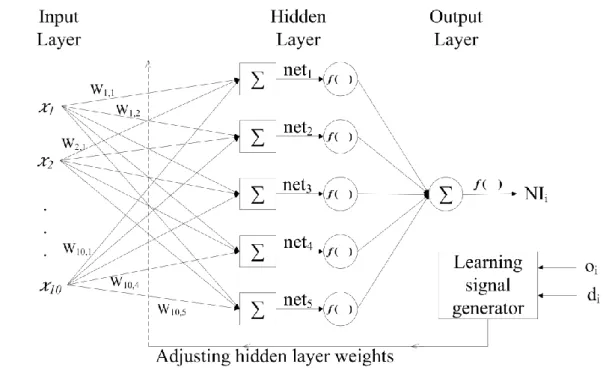
The second part is the load prediction information from a neural network-based load predictor. We used the delta learning rule in our ANN design (see Figure 8 and

Figure 8 Schematic representation of an artificial neural network model for VMi.

15

Figure 9) because the neural network has the capability of optimization and prediction. Due to there is no certain mathematical approach for obtaining the optimum number of hidden layers and their neurons [14], we used a single hidden layer for less computation time in our design.

In Figure 8, input 𝑥 is a vector which contains recent ten history weights. To avoid SLA violations, such as the response time required (di), which is specified in the SLA ,

we consider the response time when training the neural network. The neural network will calculate a weight for each VMi, which we call neural indexi (NIi). Request

Scheduler allocates requests according to NIi, and then measure the average response

time (oi). When the current average response time is close to the certain proportion

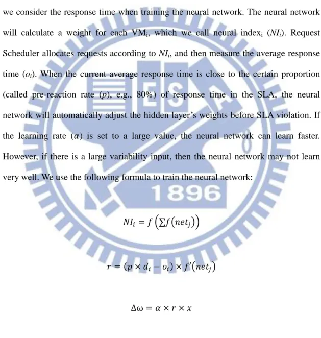
(called pre-reaction rate (p), e.g., 80%) of response time in the SLA, the neural network will automatically adjust the hidden layer’s weights before SLA violation. If the learning rate (𝛼) is set to a large value, the neural network can learn faster. However, if there is a large variability input, then the neural network may not learn very well. We use the following formula to train the neural network:

𝑁𝐼_𝑖 = 𝑓 (∑𝑓(𝑛𝑒𝑡_𝑗))

𝑟 = (𝑝 × 𝑑_𝑖 − 𝑜_𝑖) × 𝑓′(𝑛𝑒𝑡_𝑗)

∆ω = 𝛼 × 𝑟 × 𝑥

16

If there are n VMs in a local load balancer, the Weight Adjustment module will combine remaining capacity system real time information CI and neural network output NI together to calculate weighti (Wi) for VMi by following formula:

𝑊𝑖 =

𝐶𝐼𝑖 × 𝑁𝐼𝑖

∑𝑛 (𝐶𝐼_𝑗× 𝑁𝐼_𝑗)

𝑗=1

∗ 100%

Wi reflects the remaining resources proportion of VMi in the entire n VMs. The

Weight Adjustment module sends these weights to Request Scheduler. Figure 8 shows the flowchart of our algorithm.

17

18

Chapter 4

Evaluation and Discussion

4.1 Experimental environment

We built a testbed that includes a local load balancer and a VM configuration, as shown in Figure 10. This testbed was for hosting a web page service. There was three active VMs (VM1, VM2, and VM3) with different capabilities and two spare VMs

(VMs1 and VMs2), which were running in an apache web server in a virtual zone. We

used the load balancer to link these VMs together to form a virtual zone. The load balancer would distribute user requests to three VMs according the proposed scheduling algorithm nn-dwrr. The experimental environment setup and related parameters are shown in Table 3 and the configuration of the five VMs is shown in Table 4.

19

We used this testbed to host web services, and evaluated average response time using an apache benchmark (ab) to collect real web traffic for different load balancing algorithms. Requests are based on a real web service. We then compare four different scheduling algorithms.

4.2 Comparison of different load balancing

algorithms

How to utilize the advantage of cloud computing and make each task to obtain the required resources in the shortest time is an important topic [9]. Therefore, we use

Table 3. Load balancing experimental parameters. OS CentOS 5.5 Virtual machine hypervisor Xen

Number of VMs 3 Number of spare VMs 2

Application Web service Duration (time limit) 60 sec Response time specified in the SLA 2000, 1000, 432 ms

Pre-reaction rate (p) 80% Transfer function (f)

(for hidden and output layers) Log-sigmoid Learning rate (𝛼) 0.5

Table 4. Configuration of each VM.

VM1 VM2 VM3 VMs1 VMs2

CPU (cores) 1 2 3 2 2 Memory (MB) 512 1024 2048 1024 1024 Virtual disk (GB) 10 10 10 10 10 Static weight (wrr) 1 2 4 - -

20

the average response time as a metric for comparing different scheduling algorithms.

Figure 12. Comparison of four scheduling algorithms (maximum response time specified in the SLA: 2000 ms).

Figure 13. Average response time (maximum response time specified in the SLA: 2000 ms).

21

Figure 12 shows the comparison of four scheduling algorithms. The response time requirement specified in the SLA is 2000 ms. In Figure 12, we found that the static scheduling algorithm (wrr) has the longest response time. The capacity-based

Figure 14. Comparison of four scheduling algorithms (maximum response time

specified in the SLA: 1000 ms).

Figure 15. Comparison of four scheduling algorithms (maximum response time

22

and wrr scheduling algorithm has near the same performance before number of requests over 510. After that, the disparities of the response time between them will become more obvious. The performance of the ANN is good when the number of requests is large. However, we found the average response time of the ANN-based algorithm is the worst and changes greatly before the average response time exceeding 80% (pre-reaction rate) of the response time specified in the SLA. This is because the ANN-based algorithm will continue to distribute requests to a VM when the response time not exceeding 80% of the response time specified in SLA. Disregarding the number of requests, the performance of the proposed nn-dwrr is always the best. Figure 13 shows that the proposed nn-dwrr is 1.86 times faster than wrr, 1.49 times faster than capacity-based, and 1.21 times faster than ANN-based scheduling algorithms in terms of average response time. Figure 14 and Figure 15 shows the cases under different response times (1000 ms and 432 ms) specified in the SLA. They shows the performance differences of the ANN-based and nn-dwrr are getting closer when the specified response time become smaller.

23

4.3 Comparison of SLA violation rates with and

without a spare VM pool

Figure 16 shows the comparison of the SLA violation rate with and without a spare VM pool in the proposed tldlb architecture, both running the proposed nn-dwrr algorithm. In this experiment, the threshold of the SLA violation rate was set to 5%. The SLA violation rate is defined as follows:

SLA violation rate =Number of requests violated Number of total requests

The SLA Engine, as shown in Figure 7, will keep monitoring the response time of each request and calculating the SLA violation rate. The SLA Engine would activate a spare VM when the SLA violation rate exceeds its threshold (5%, in this case). We found that the proposed tldlb can avoid exceeding the SLA violation rate of 5% by activating VMs from a spare VM pool. The proposed tldlb can indeed reduce the SLA violation rate by activating VMs in the spare VM pool in time.

24

Chapter 5

Conclusion

5.1 Concluding remarks

We have presented an SLA-aware decentralized load balancer architecture, tldlb, which can reduce the SLA violation rate. If active VMs are overloaded, the proposed tldlb avoids SLA violations by activating spare VMs in a spare VM pool. In addition, we also proposed a novel neural network-based load balancing algorithm, nn-dwrr, to distribute incoming requests to appropriate VMs. Experimental results have shown that the proposed nn-dwrr is 1.86 times faster than the wrr, 1.49 times faster than the capacity-based, and 1.21 times faster than the ANN-based scheduling algorithms, in terms of average response time. The experiment results have demonstrated that our proposed nn-dwrr algorithm has faster response time, which means we can handle more requests per second. Since our scheduling algorithm is simple and efficient, it is well-suited for cloud computing environments to service a large number of requests with less response time.

5.2 Future work

In our current design, we focused only on the local load balancer. In the future, we will implement the global load balancer and will conduct some experiments to evaluate user requests redirection performance. In addition, we will deploy our load balancers to a cloud datacenter testbed for further evaluation.

25

References

[1] “Cloud Computing – Wiki,” [Online]. Available: http://en.wikipedia.org/wiki/Cloud_computing/.

[2] “Amazon S3 Growth,” [Online]. Available: http://www.datacenterknowledge.com/wp-content/uploads/2011/01/amazon-s3_gr owth_2010.jpg/.

[3] Z. Zhang and X. Zhang, "A Load Balancing Mechanism Based on Ant Colony and Complex Network Theory in Open Cloud Computing Federation," in Proceedings of International Conference on Industrial Mechatronics and Automation (ICIMA), pp. 240-243, 2010.

[4] W. Y. Lin, G. Y. Lin, and H. Y. Wei, "Dynamic Auction Mechanism for Cloud Resource Allocation," in Proceedings of Cluster, Cloud and Grid Computing (CCGrid), pp. 591-592, 2010.

[5] “Amazon Elastic Load Balancing,” [Online]. Available: http://aws.amazon.com/elasticloadbalancing.

[6] “rackspace - Cloud Load Balancers On-Demand,” [Online]. Available: http://www.rackspace.com/cloud/cloud_hosting_products/loadbalancers.

[7] “Service-level agreement – Wiki,” [Online]. Available: http://en.wikipedia.org/wiki/Service-level_agreement.

[8] R. Rajavel, “De-Centralized Load Balancing for the Computational Grid environment,” in Proceeding of International Conference on Communication and Computational Intelligence (INCOCCI), pp. 419-424, Dec. 2010.

[9] S. C. Wang, K. Q. Yan, W. P. Liao, and S. S. Wang, “Towards a Load Balancing in a Three-level Cloud Computing Network,” in Proceeding of IEEE International

26

Conference on Computer Science and Information Technology (ICCSIT), vol. 1, pp. 108-113, Jul. 2010.

[10] “Linux Virtual Server,“ [Online]. Available: http://www.linuxvirtualserver.org. [11] M. Randles, D. Lamb, and A. Taleb-Bendiab, “A Comparative Study into

Distributed Load Balancing Algorithms for Cloud Computing,” in Proceeding of Advanced Information Networking and Applications Workshops, pp. 551-556, Apr. 2010.

[12] C. C. Li, and K. Wang, “SLA-aware Load Balancing for Cloud Data Centers,” Report, 2012.

[13] V. Nae, A. Iosup, and R. Prodan, “Dynamic Resource Provisioning in Massively Multiplayer Online Games,” IEEE Transactions on Parallel and Distributed Systems, vol. 22, no. 3, pp. 380-395, Mar. 2011.

[14] Y. Zhang, J. Pang, R. Zhao, and Z. Guo, "Artificial Neural Network for Decision of Software Maliciousness", in Proceedings of Intelligent Computing and Intelligent Systems (ICIS), pp. 622-625, 2010.

[15] J. Hu, J. Gu, G. Sun, and T. Zhao, “A Scheduling Strategy on Load Balancing of Virtual Machine Resources in Cloud Computing Environment,” in Proceedings of International Symposium on Parallel Architectures, Algorithms and Programming (PAAP), pp. 89-96, Dec. 2010.