Subwavelength spatial solitons of TE mode

1 December 1998

Ž .

Optics Communications 157 1998 170–172

Subwavelength spatial solitons of TE mode

Chi-Feng Chen, Sien Chi

)

Institute of Electro-Optical Engineering, National Chiao Tung UniÕersity, Hsinchu 30050, Taiwan Received 6 April 1998; revised 15 July 1998; accepted 11 September 1998

Abstract

The wave equation of TE subwavelength beam propagations in a nonlinear planar waveguide is derived. This equation contains more higher-order linear and nonlinear terms than the nonlinear Schrodinger equation. The analytic solution of TE

¨

subwavelength spatial soliton is found to be the same as the conventional spatial soliton in amplitude but different in phase. The numerical results show that the analytic solution is stable. q 1998 Elsevier Science B.V. All rights reserved.

Keywords: Nonlinear effect; Spatial soliton; Nonlinear planar waveguide

1. Introduction

Spatial solitons in a nonlinear planar waveguide due to the balance of the diffraction and the self-focusing have

w x

been studied both theoretically and experimentally 1,2 . The propagation of spatial solitons are commonly

de-Ž .

scribed by the nonlinear Schrodinger equation NSE which

¨

is derived by making the paraxial approximation. How-ever, when a beam width is as narrow as one wavelength or less the validity of the paraxial approximation becomes questionable. To resolve this problem, the full-vector

non-w x

linear Maxwell’s equations was solved 3,4 , but it is very time consuming. In addition, some researchers suggest considering the additional terms in NSE to enhance the

w x

validity of the wave equation 5,6 . It is shown that when the additional terms including a polarization-dependent correction to the soliton propagation constant exists, the dynamics of a narrow spatial soliton with an arbitrary

w x

polarization will be influenced 5 . By using the wave

w x

equation of TM mode in Ref. 5 , they analyze the effects of those addition terms on the shapes of bright and dark

w x

solitons of TM mode with a fixed polarization 6 . In this paper, we will derive the propagation equation for a TE subwavelength beam in a nonlinear planar

wave-)

Corresponding author. E-mail: schi@cc.nctu.edu.tw

w x

guide by the iteration method 7 . The derived equation contains more higher-order linear and nonlinear terms than the NSE. An analytic solution of the subwavelength spatial soliton of TE mode can be found and the numerical results show that this analytic solution is stable.

2. Derivation of the wave equation

We now derive the wave equation which can describe the propagations of subwavelength beams of TE mode in a nonlinear planar waveguide. The electric field E of the light obeys the vector wave equation

v2_n2 _v2 ₁

0 2

= E y 2 E q 2 PNLq 2 = = P P

Ž

NL

.

s0,

Ž .

1

c c ´0 n ´0 0

where ´0 is the vacuum permittivity, n0 is linear refrac-tive index, v is the light frequency, c is the velocity of light in vacuum, and P_NL is the third-order nonlinear polarization and 3´₀ Ž3. ) P s x

Ž

v s v q v y v

.

E E E ,

Ž

NL

.

i

_Ý

i , j, k , l j k l j k l 4 _{j, k , l} Ž3. Ž .

where x v is the third-order susceptibility, i, j, k, and

l refer to the Cartesian components of the fields.

0030-4018r98r$ - see front matter q 1998 Elsevier Science B.V. All rights reserved. Ž .

( )

C.-F. Chen, S. Chi r Optics Communications 157 1998 170–172 171

For a TE mode of the planar waveguide, we consider the propagation of one-dimensional beam along z-direc-tion with a uniform field in the y-direcz-direc-tion. The electric

w x

field of the light can be taken as 5

E x , z s yA

Ž

.

ˆ

y

Ž

x , z exp ik z ,

.

Ž

0

.

Ž .

2

Ž . Ž .

where A_y x, z is the envelope and k s n vrc is the_{0 0}

propagation constant. The total refractive index is given by

< <2 _{< <}2

n s n q n E s n q n0 2 0 2 Ay , where n is the Kerr co-2

Ž (3) .

efficient and n s 3x_{2 y y y y}r8 n .₀

Ž . Ž .

Substituting Eq. 2 into Eq. 1 , we obtain

E 1 E2 _{1 E}2 2 < < i_{E z}A qy _{2 k E x}2A q g Ay y A s yy _{2 k E z}2Ay

Ž .

3 0 0 Ž .

where g s k n rn . To normalize Eq. 3 , we make the0 2 0

following transformations: P

'

0 n0 Ay

Ž

x , z s

.

u h ,j s s

Ž

.

(

u h ,j ,

Ž

.

Ž

4a

.

N n2 x s w h ,0

Ž

4b

.

z s L jd

Ž

4c

.

wŽ . Ž 2 2 .x1r2

where the parameter N s n P r k w n_{2 0 0 0 0} is the order of the spatial soliton and N s 1 for the fundamental soliton, w s w r1.763 and w is the full width at the half_{0 F F}

Ž .

maximum FWHM of the beam, P is peak power of the0

Ž .

incident beam, the parameter s s 1rk w s 0.28 l rw0 0 0 F

and l s 2prk_{0 0} is the wavelength of the light in the waveguide, and L s k w2 _{is the diffraction length. By}

d 0 0

Ž . Ž . Ž . Ž .

using Eqs. 4a , 4b and 4c , Eq. 3 can be normalized to: E _{i E}2 _is2 _E2 2 < < u s ₂u q i u u q ₂u.

Ž .

5 Ej 2 Eh 2 Ej 3. Iterative method

Now we use the iterative method to replace the second

Ž 2 2.

derivative E rEj u term by the higher order diffraction

Žlinear and nonlinear terms, such that the wave equation.

can be simplified without making the paraxial

approxima-Ž 2 2.

tion. First, neglecting the second derivative E rEj u in

Ž .

Eq. 5 and assigning the equation remaining as the wave equation of the zero order approximation:

E u sH ,

Ž .

6

ž /

Ej ₀ where i E2 ₂ < < H s ₂u q i u u.

Ž .

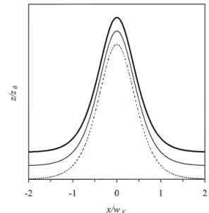
7 2 Eh

Fig. 1. Power evolution of the beam shape for the TE soliton at Žz r z s 0 dashed curve , z r z s10 solid curve , z r z s0. Ž . Ž 0. Ž . Ž 0.

Ž .

20 thick solid curve .

which is the well-known NSE for spatial soliton

propaga-Ž .

tions. By differentiating Eq. 6 with respect to j , the

Ž 2 2.

second derivative E rEj u can be approximated to:

E2 _{E H}

u s ,

Ž .

8

2

ž

Ej

/

Ej

1

which is assigned as the first order approximation.

Substi-Ž . Ž .

tuting Eq. 8 into Eq. 5 , we obtain the wave equation of the first order approximation:

E u is2 _E2

sH q 2u .

Ž .

9

ž /

Ej ₁ 2

ž

Ej

/

1

The process repeats until the expression of the second

Ž 2 2.

derivative E rEj u does not change for the required

order, so that we can obtain an accurate wave equation that includes only the first distance derivative without making the paraxial approximation.

If we only take into account up to terms of the order of

2 _Ž 2 2_.

s , the second derivative E rEj u does not change after

one iteration: 2 2 4 2 E _{1 E E u E u} 2 ) < < u s y u y 2 u y u 2 4 2

ž /

ž

Ej

/

4 Eh

ž /

Eh Eh 1 2 E u ₄ < < y2 _Eh u y u u.

Ž

10

.

( ) C.-F. Chen, S. Chi r Optics Communications 157 1998 170–172 172

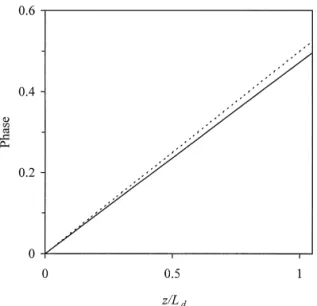
Fig. 2. The phase versus propagation distance for the TE soliton

Ž .

with higher-order terms solid curve and without higher-order

Ž .

terms dashed curve .

Ž . Ž .

Substituting Eq. 10 back into Eq. 5 , we obtain the wave equation of the second order approximation:

2 2 4 E u i E ₂ s 1 E < < s _{u q i u u q i} y _u 2 4 Ej 2 Eh 2 4 Eh 2 2 2 E u ₂ E u E u ₄ ) < < < < y_{2 u y u y 2 u y u u .} 2

ž /

ž /

Eh Eh Eh 11

Ž

.

For higher-order approximation, we should have s4_r4

terms. These terms are much smaller than s2_{r2 terms} 2

Ž . 2

when s r2 < 1. Therefore, Eq. 11 is valid when s r2 is sufficient smaller than unit.

4. Solution and discussion

Ž .

We have found that the Eq. 11 has a spatial soliton solution and it is:

u j ,h s sech h exp idjr2 ,

Ž

.

Ž .

Ž

.

Ž

12

.

Ž 2 .

where d s 1 y s r4 . To numerically simulate the

soli-Ž .

ton propagation governedly that Eq. 11 is indeed an exact

Ž . 2

solution for Eq. 11 , we take w s 0.6l , i.e., s r2 fF 0

Ž .

0.1. We use split-step Fourier method to solve Eq. 12 . Fig. 1 shows the evolution of the pulse shape for spatial soliton of TE mode in a nonlinear planar waveguide. It is seen that the beam propagates undistortedly over 20 z ,0

Ž .

and z s pr2 L is the spatial soliton period. In Fig. 2,_{0 d} we show the phase versus propagation distance. The change of this phase is consistent with the analytic result. There-fore, the analytic soliton with a modified phase in a soliton solution.

5. Conclusion

In conclusion, we have derived an accurate wave equa-tion from the Maxwell’s equaequa-tions beyond paraxial ap-proximation by the iterative method for the subwavelength optical beam propagation in a nonlinear planar waveguide. The derived equation of the TE mode contains more higher-order linear and nonlinear terms than the nonlinear Schrodinger equation. We have found an analytic spatial

¨

soliton solution from the derived equation, and the ampli-tude of spatial soliton is the same as that of the conven-tional spatial soliton but its phase becomes smaller. The numerical results show that this spatial soliton is stable for the subwavelength optical beam propagation in a nonlinear planar waveguide.

Acknowledgements

The work is partially supported by National Science Council, Republic of China, under Contract NSC 87-2215-E-009-014.

References

w x1 A. Hasegawa, F. Tappert, Appl. Phys. Lett. 23 1973 142.Ž . w x_{2 J.S. Aitchison, A.M. Weiner, Y. Silberberg, M.K. Oliver, J.L.}

Jackel, D.E. Leaird, E.M. Vogel, P.W.E. Smith, Opt. Lett. 15 Ž1990 471..

w x_{3 R.M. Joseph, A. Taflove, IEEE Photon. Technol. Lett. 6} Ž1994 1251..

w x4 C.V. Hile, W.L. Kath, J. Soc. Am. B 13 1996 1135.Ž . w x5 A.W. Snyder, D.J. Mitchell, Y. Chen, Opt. Lett. 19 1994Ž .