以基因演算法研究三點式非再生性MIMO中繼站系統之最佳Precoder Pair

(1)

國立交通大學

電信工程學系碩士班

碩士論文

以基因演算法研究三點式非再生性

MIMO 中繼站系統之最佳 Precoder Pair

Generic Algorithm Based Optimal Precoder Pair for

Three-terminal Non-regenerative MIMO Relay System

研究生：劉丞瑋

指導教授：沈文和博士

(2)

以基因演算法研究三點式非再生性

MIMO 中繼站系統之最佳 Precoder Pair

Generic Algorithm Based Optimal Precoder Pair for

Three-terminal Non-regenerative MIMO Relay System

研究生 : 劉丞瑋 Student : Cheng-Wei Liu

指導教授 : 沈文和博士 Advisor : Dr. Wern-Ho Sheen

國立交通大學

電信工程學系碩士班

碩士論文

A Thesis

Submitted to Department of Communication Engineering

College of Electrical and Computer Engineering

National Chiao Tung University

in Partial Fulfillment of the Requirements

for the Degree of

Master of Science

in Communication Engineering

October 2008

Hsinchu, Taiwan, Republic of China

中華民國九十七年十月

(3)

以基因演算法研究三點式非再生性

MIMO 中繼站系統之最佳 Precoder Pair

研究生:劉丞瑋指導教授:沈文和博士

國立交通大學

電信工程學系碩士班

摘要

為了增加現有系統的覆蓋範圍及link level 之通道容量以達到更高的系統需求，中繼站系統是一個在新一代通訊系統下可能被採用的架構。而MIMO Precoding 這門技術目前也被廣泛的應用在中繼站系統來進一步改善系統效能。然而，目前的研究大多著眼於兩躍式中繼站系統之中繼站端precoder 設計。在本論文中作者將透過基因演算法來研究由來源端precoder 及中繼站端 precoder 所構成之 precoder pair。對一個可應用多種兩段式傳送規約之三點式非再生性 MIMO 中繼站系統而言，數值分析結果顯示，相對於沒有precoder pair 的中繼站系統，precoder pair 可在相同的總傳送功率限制之下提升ergodic/outage capacity。

(4)

Generic Algorithm Based Optimal Precoder Pair for

Three-terminal Non-regenerative MIMO Relay Channel

Student : Cheng-Wei Liu

Advisor : Dr. Wern-Ho Sheen

Department of Communication Engineering

National Chiao Tung University

Abstract

Relay system is a possible candidate to be adopted in the next generation

communication systems. It aims to enhance the coverage and link level capacity of current systems. Also, the technique of MIMO precoding has been widely applied onto relay systems to further improve system performance. However, most previous

researches focus on designing the relay precoder matrix for two-hop MIMO relay systems. In this thesis, precoder pair, which consists of relay precoder matrix and an additional source precoder matrix, has been studied based on the classical Generic algorithm. For MIMO relay systems with various two-phase transmission protocols, numerical results show that ergodic/outage capacity improvement with respect to traditional techniques can be achieved with guaranteed individual transmit power constraint for source and relay terminals.

(5)

誌謝

首先感謝沈文和教授在碩士班這兩年給我的指導與栽培。老師教導我凡事要有邏輯性的思考，不要相信常規;並且告訴我們做事就要做到完美，不要輕易妥協，我相信這些觀念對於我將來在社會上工作時一定會有莫大的幫助。此外，有許多學長的協助與建議，得以讓我的研究順利進行。在此感謝東融、宸睿、聖文、倉緯等學長們，他們不僅僅在課業上給予建議，私底下我們也成為好朋友，相信這段友情不會隨著畢業的到來而淡去。而和我一起努力的同學，政揚、宜勳、哲群，我們不僅互相討論研究，更互相扶持成長，期待彼此都能在社會上有一番好成就。特別要感謝一些總是支持我的人，小台、小又、筱涵、怡利、怡萱。最後，我要感謝我的家人。爸爸、媽媽、妹妹，謝謝你們。民國九十七年十月研究生劉丞瑋謹識於交通大學

(6)

List of Figures

Fig. 2.1: Linear precoding system block diagram... 6

Fig. 2.2: Linear precoder structure using SVD... 7

Fig. 3.1: Comparison of the searching points for GA and gradient technique... 21

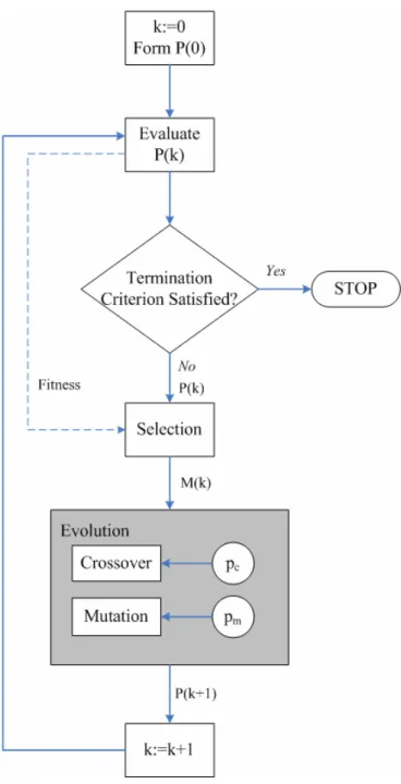
Fig. 3.2: Flow chart of Generic algorithm ... 23

Fig. 4.1: Three-Terminal MIMO Non-regenerative Relay System Block... 25

Fig. 4.2(a): The first phase of TD protocol ... 28

Fig. 4.2(b): The second phase of TD protocol... 28

Fig. 4.3(a): The first phase of RD protocol ... 29

Fig. 4.3(b): The second phase of RD protocol ... 30

Fig. 4.4(a): The first phase of STD protocol ... 31

Fig. 4.4(b): The second phase of STD protocol ... 31

Fig. 4.5(a): The first phase of MH protocol ... 32

Fig. 4.5(b): The second phase of MH protocol ... 33

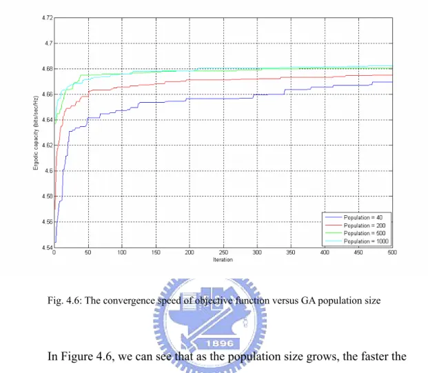
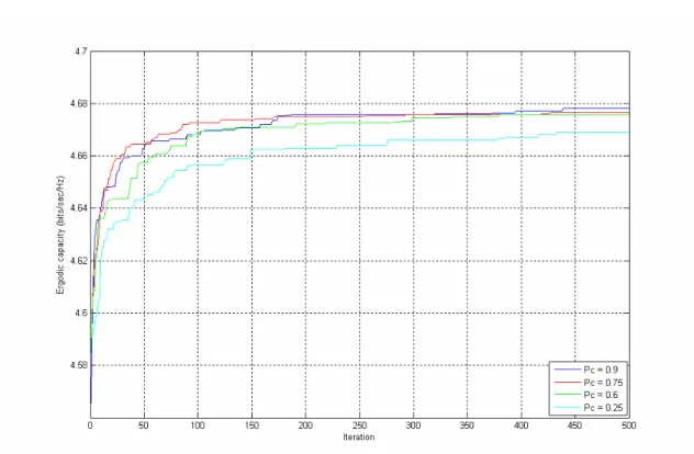
Fig. 4.6: The convergence speed of objective function versus GA population size 39 Fig. 4.7: The convergence speed of objective function versus crossover rate... 40

Fig. 4.8: The convergence speed of objective function versus mutation rate ... 41

Fig. 5.1: Numerical result 1... 46

Fig. 5.11: Numerical result 11 ... 59

(9)

(10)

List of Tables

(11)

Chapter 1 Introduction

The origin of relay systems can be traced back to the seventies [1] [2]. Recently, relay functionalities and relaying strategies have become a major topic in the wireless research community again due to its essential to provide reliable transmission, high link level capacity and broad coverage for wireless networks in a variety of applications.Moreover, these networks are typically employed in fading environments, rendering the transmitted signals vulnerable to severe attenuations in their received strength. In a cellular environment, a relay can be deployed in areas where there are strong shadowing effects, such as inside

buildings and tunnels. For mobile ad hoc networks, relaying is essential not only to overcome shadowing due to obstacles but also to reduce unnecessary transmission power from source and hence radio frequency interference to neighboring

terminals. In such settings, it becomes necessary for the terminals in the network to cooperate at the physical layer in order to increase the link level capacity between any pair of terminals and to ensure robustness of the communications to changes in channel conditions. As a result, precoding, a MIMO (multiple-input multiple-output) signal processing technique that based on the channel state information (CSI), is applied onto relay systems to further improve system performance. The unit executes precoding is called precoders.

Relay precoder design criterion varies in many ways, including:

Ergodic capacity, achievable rate, and mutual information [3] ~ [9]. MSE or SNR at receiver side [10] ~ [12].

(12)

Diversity gain [13].

Outage probability and achievable outage rate [14].

For example, in [4], the author proved that the optimal relay precoder matrix has a unique form and proposed an optimal relay power loading matrix to

maximize the two-hop MIMO non-regenerative channel ergodic capacity; In [9], the author proposed a power allocation algorithm for both source and relay terminals while the MIMO channel has been parallelized by the precoder pair; In [10], with statistical CSIT and perfect CSIR, the author derived the optimal power allocation that minimizes high- SNR approximations of the outage probability; In [11], the author developed a generalized notion of SNR (GSNR) for a two-hop SISO relay channel and proposed the so-called estimate and forward relaying and its corresponding relay precoder which maximizes GSNR.

Most previous researches focus on relay precoder design and hence problems arise: What if we have an additional precoder at source terminal? What is the joint optimal precoder pair of such three-terminal MIMO relay channel its impact to the system performance? To answer these problems, we are going to find the optimal precoder pairs for various network configurations and their corresponding

performance limits of a three-terminal MIMO non-regenerative relay channel.

The following chapters are composed as below: Chapter 2 contains

background knowledge of MIMO wireless precoding, and we will introduce basic elements of Generic algorithm in Chapter 3; the system model, two-phase

(13)

implementation together organize the main body of this thesis, is placed in Chapter 4; Chapter 5 shows simulation results and corresponding observations, and

(14)

Chapter 2 MIMO Wireless Precoding

2.1 Introduction

Precoding is a generalized beamforming scheme to support

multi-layer(multiple data streams) transmission in MIMO radio systems. Conventional beamforming considers linear single-layer precoding so that the same signal is emitted from each of the transmit antennas with appropriate

weighting such that the received signal power is maximized at the receiver. When the receiver has multiple antennas, the single-layer beamforming can not

simultaneously maximize the received signal power at all of the receive antennas and so precoding is used for multi-layer beamforming in order to optimize the performance index such as maximize the achievable rate of a multiple receive antenna system. In other words, the signals of the multiple data streams are

emitted from the transmit antennas with independent and appropriate weighting on each antenna such that the performance index is optimized.

So it is clear that precoding design is to find the appropriate weightings, which depending on the available CSIT (channel state information at transmitter side) and the performance index we interest in. CSIT usually comes from the feedback of receiver. However, when the feedback delay is greater than the channel coherence time, no estimate is valid and we can only rely on statistical information, such as channel mean and covariance. These statistics can be reliably obtained by averaging channel measurements over multiple channel coherence times. Different performance indexes will also lead to different precoding design.

(15)

Precoders can also be designed to minimize the error probability, minimize the outage probability, minimize the detection mean squared-error (MSE), maximize the ergodic capacity, or maximize the received signal-to-noise ratio (SNR). These different precoder designs can be analyzed using the common linear precoding structure.

In the remaining of this chapter we will focus on linear precoding with perfect CSIT. First, a basic system linear precoding block diagram will be

presented; and then we will give an intuitive explanation for the power constraints and some common design criteria.

2.2 Linear precoding system

All communication systems can be seen as the composition of three parts: the transmitter, the channel, and the receiver. Since the precoder is part of the

transmitter side, we will pay attention to the transmitter.

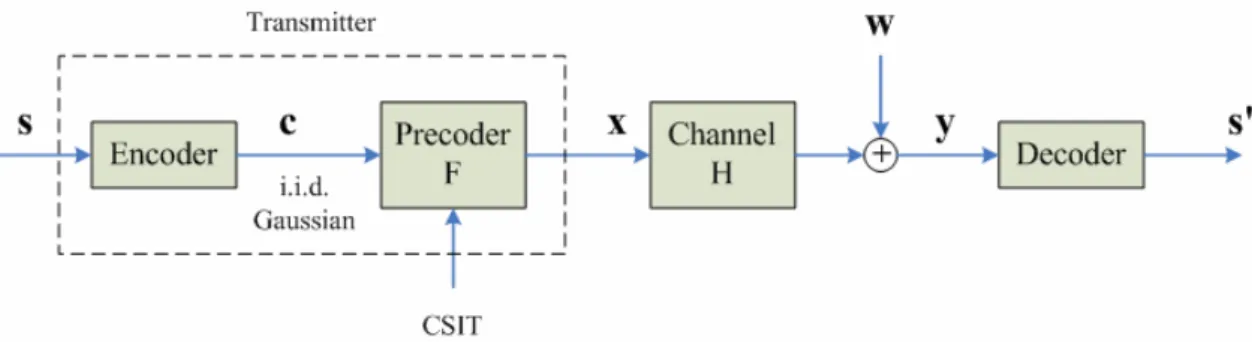
The transmitter in a system with linear precoding consists of a channel encoder and a precoder is presented in Figure 2.1. The channel encoder takes data streams s in and performs necessary coding for error correction by adding

redundancy, then maps the coded bits into symbol vectors c. The precoder processes these symbols before transmission from the antennas and produces the transmitted signal x. At the other side, the receiver decodes the noise-corrupted received signal y to recover the data bits s’. If the input-output relation of a system with a precoder at transmitter side can be expressed as

(16)

y = HFc + w

(2—1)

than this system can be referred to a linear precoding system. In the next chapter, the structure of common linear precoder will be further investigated.

Fig. 2.1: Linear precoding system block diagram

2.2.1 Basic linear precoder structure

Basic linear precoder functions as a combination of an input signal shaper and a multi-mode (multi-subchannel) beamformer with per-beam power allocation. Consider the singular value decomposition (SVD) of the precoder matrix F:

F =U

F

D

F

V

FH (2—2)

The orthogonal beam directions are the left singular vectors UF, of which each column represents a beam direction, so UF is often called a multi-mode

beamformer. Note that UF is also the eigenvectors of the product FFH, thus UF is also referred to as eigen-beamformer. The beam power loadings are the squared singular values DF. The right singular vectors VF mix the precoder input symbols

c

to feed into each beam direction and hence is referred to as the input shaping matrix. This structure is illustrated in Figure 2.2.

(17)

Fig. 2.2: Linear precoder structure using SVD

Essentially, a precoder has two effects: decoupling the input signal into orthogonal spatial modes (subchannels) in the form of eigen-beams, and allocating power over these beams based on the CSIT. If the precoded orthogonal spatial beams perfectly match the channel eigen-directions (the eigenvectors of HHH),

there will be no interference among signals sent on different modes, thus creating parallel channels and allowing transmission of independent signal streams. This effect, however, requires the full channel knowledge at the transmitter. With partial CSIT, the precoder performs its best to approximately match its

eigen-beams to the channel eigen-directions and therefore reduces the interference among signals sent on these beams. This is the decoupling effect. Moreover, the precoder allocates power on the beams. By allocating power, the precoder effectively matches the channel based on the CSIT, so that more power is sent in the directions where the channel is strong and less or no power in the weak.

2.2.2 Power constraint

In precoder design, power constraints are necessary to avoid trivial solutions such as increasing the norm of the precoder matrix to infinity, which is impossible practically. In this section, we are going to introduce some common power

(18)

A reasonable power constraint is obtained by bounding the expected norm of the transmit vector

{ }

2

(

_H

)

E

x

=

tr

FF

_,_(2—3)

which limits the total transmit power, and thus, we will refer this power constraint as:

{ }

2

( )

_H

E

x

=

tr

FF

≤

P

_._(2—4)

An alternative is to constrain the maximum eigenvalue of the transmit vector covariance matrix FFH, which also limits the power because

(

H

)

(

)

max

tr

FF

≤

Nλ

FF

H _,_(2—5)

where N is the number of nonzero eigenvalues of FFH. This corresponds to

(

H

)

max

Nλ

FF

=

P

. (2—6) Besides limiting the transmit power, the maximum eigenvalue constraint imposes a limit on the peak power of the output signal. The advantage of this constraint is that it limits the signal peak, independent of the specific constellation used. The disadvantage is that the bound may not be tight.

In relay system, one issue about power constraint is that besides the

individual power constraint for source terminal and relay terminal, the total power dissipated by source and relay terminals should be constrained or not. We do not impose this constraint because in a practical system the source terminal and the relay terminal have independent power supplies.

(19)

2.2.3 Precoder design criteria

There are alternate precoding design criteria based on both fundamental and practical performance indexes. The fundamental performance indexes include the ergodic capacity and the error probability, while the practical performance indexes contain, for example, the outage probability, mean square-error (MSE), and the received SNR. The choice of the design criterion depends on the system setup, operating parameters, and the channel (fast or slow fading). For example, fundamental performance indexes usually assume ideal channel coding; the ergodic capacity implies that the channel evolves through all possible realizations over arbitrarily long codewords, while the error probability applies for finite codeword lengths; on the other hand, analyses using practical performance indexes usually apply to uncoded systems and assume a block fading channel.

(20)

Chapter 3 Generic Algorithm

3.1 Introduction

John Holland, from the University of Michigan began his work on genetic algorithms at the early 60s. A first achievement was the publication of Adaptation

in Natural and Artificial System in 1975.

Holland had a double aim: to improve the understanding of natural adaptation process, and to design artificial systems having properties similar to natural

systems. Since then, generic algorithms have been used widely as a tool in computer programming and artificial intelligence, optimization, neural network training, and many other areas.

The basic idea is as follow: the genetic pool of a given population potentially contains the optimal solution, or a better solution, to a given adaptive problem. This solution is not "active" because the genetic combination on which it relies is split between several subjects. Only the association of different genomes can lead to the solution.

Holland’s method is especially effective because he not only considered the role of mutation, but he also utilized genetic recombination: the crossover of partial solutions greatly improves the capability of the algorithm to approach, and eventually find, the optimum solution.

(21)

3.2 Basic Concepts

The principle of genetic algorithms is presented below:

A. Random generation of a population. This one includes a genetic pool containing a group of possible solutions.

B. Encoding of the population members in corresponding binary strings. Each binary string is called a chromosome which contains multiple genes (bits).

C. Reckoning of the fitness value, the objective function value we want to optimize, for each subject. The fitness value will directly depend on the distance to the optimum solution.

D. Selection of the subjects that will mate according to their share in the population global fitness.

E. Genomes crossover and mutations. F. Start again from point C.

In the next couple of sections, we introduce some generic operators and their corresponding implement methods in detail.

3.2.1 Selection

Selection is a genetic operator that chooses a chromosome from the current generation’s population for inclusion in the next generation’s population. Before making it into the next generation’s population, selected chromosomes may undergo crossover and/or mutation (depending upon the probability of crossover and mutation, Pc and Pm) in which case the offspring chromosome(s) are actually the ones that make it into the next generation’s population. Common selection

(22)

methods are:

Roulette

A selection operator which the chance of a chromosome getting selected is proportional to its fitness value. This is where the concept of survival of the fittest comes into play.

Tournament

A selection operator which uses roulette selection N times to produce a tournament subset of chromosomes. The best chromosome in this subset is then chosen as the selected chromosome. This method of selection applies addition selective pressure over plain roulette selection.

Top Percent

Top percent is a selection operator which randomly selects one chromosome from top N percent of the current population, where N is previously specified by user.

Best

It’s a selection operator which selects the best chromosome (as determined by fitness value). If there are two or more chromosomes with the same best fitness, one of them is chosen randomly.

Random

It’s a selection operator which randomly selects a chromosome from the population.

(23)

3.2.2 Crossover

Crossover is a genetic operator that combines (mates) two chromosomes (parents) to produce new chromosome(s) (offspring). The idea behind crossover is that the new chromosome(s) may be better than both of the parents if it takes the best characteristics from each of the parents. Crossover occurs during evolution according to a user-definable crossover probability. Followings are some common methods to implement crossover:

One Point

A crossover operator that randomly selects a crossover point within a chromosome then interchanges the two parent chromosomes at this point to produce two new offspring.

Consider the following two parents which have been selected for crossover. The “|” symbol indicates the randomly chosen crossover point.

Parent 1: 11001|010 Parent 2: 00100|111

After interchanging the parent chromosomes at the crossover point, the following offspring are produced:

Offspring1: 11001|111 Offspring2: 00100|010

(24)

Two Point

A crossover operator that randomly selects two crossover points within a chromosome then interchanges the two parent chromosomes between these points to produce two new offspring.

Consider the following two parents which have been selected for crossover. The “|” symbols indicate the randomly chosen crossover points.

Parent 1: 110|010|10 Parent 2: 001|001|11

After interchanging the parent chromosomes between the crossover points, the following offspring are produced:

Offspring1: 110|001|10 Offspring2: 001|010|11

Uniform

A crossover operator that decides (with some probability – known as the mixing ratio) which parent will contribute each of the gene values in the offspring chromosomes. This allows the parent chromosomes to be mixed at the gene level rather than the segment level (as with one and two point crossover). For some problems, this additional flexibility outweighs the disadvantage of destroying building blocks.

(25)

Consider the following two parents which have been selected for crossover:

Parent 1: 11001010 Parent 2: 00100111

If the mixing ratio is 0.5, approximately half of the genes in the offspring will come from parent 1 and the other half will come from parent 2. Below is a possible set of offspring after uniform crossover:

Offspring1: 1111010202121201 Offspring2: 0202120111011112

Note: The subscripts indicate which parent the gene came from.

Arithmetic

A crossover operator that linearly combines two parent chromosome vectors to produce two new offspring according to the following equations:

Offspring1 = a * Parent1 + (1- a) * Parent2 (3—1) Offspring2 = (1 - a) * Parent1 + a * Parent2 (3—2)

where a is a random weighting factor (chosen before each crossover operation).

Consider the following two parents (each consisting of 4 float genes) which have been selected for crossover:

(26)

Parent 1: (0.3)(1.4)(0.2)(7.4) Parent 2: (0.5)(4.5)(0.1)(5.6)

If a = 0.7, the following two offspring would be produced:

Offspring1: (0.36)(2.33)(0.17)(6.86) Offspring2: (0.402)(2.981)(0.149)(6.842)

Heuristic

A crossover operator that uses the fitness values of the two parent chromosomes to determine the direction of the search. The offspring are created according to the following equations:

Offspring1 = BestParent + r * (BestParent – WorstParent) (3—3) Offspring2 = BestParent (3—4)

where r is a random number between 0 and 1.

It is possible that Offspring1 will not be feasible. This can happen if r is chosen such that one or more of its genes fall outside of the allowable upper or lower bounds. For this reason, heuristic crossover has a user settable parameter n for the number of times to try and find an r which results in a feasible

chromosome. If a feasible chromosome is not produced after n tries, the WorstParent is returned as Offspring1.

Crossover is the most important part of genetic algorithms, there is nevertheless other operators like mutation and inversion. In fact, the desired

(27)

solution may happen not to be present inside a given genetic pool, even a large one. Mutations allow the emergence of new genetic configurations which, by widening the pool improve the chances to find the optimal solution. In next section we are going to introduce mutation operator.

3.2.3 Mutation

Mutation is a genetic operator that alters one ore more gene values in a chromosome from its original state. This can result in entirely new gene values being added to the gene pool. With these new gene values, the genetic algorithm may be able to arrive at better solution than was previously possible. Mutation operator is an important part of the genetic algorithms as it helps to prevent the population from stagnating at any local optimum. Mutation occurs during evolution according to a user-definable mutation probability. This probability should usually be set fairly low (0.01 is a good first choice). If it is set to high, the search will turn into a primitive random search. Followings are some common methods to implement mutation:

Flip Bit

Flip bit is a mutation operator that simply inverts the value of the chosen gene (0 goes to 1 and 1 goes to 0). This mutation operator can only be used for binary genes.

Boundary

This is a mutation operator that replaces the value of the chosen gene with either the upper or lower bound for that gene (chosen randomly). This mutation

(28)

operator can only be used for integer and float genes.

Non-Uniform

A mutation operator that increases the probability that the amount of the mutation will be close to 0 as the generation number increases. This mutation operator keeps the population from stagnating in the early stages of the

evolution then allows the genetic algorithm to fine tune the solution in the later stages of evolution. This mutation operator can only be used for integer and float genes.

Uniform

A mutation operator that replaces the value of the chosen gene with a uniform random value selected between the user-specified upper and lower bounds for that gene. This mutation operator can only be used for integer and float genes.

Gaussian

A mutation operator that adds a unit Gaussian distributed random value to the chosen gene. The new gene value is clipped if it falls outside of the

user-specified lower or upper bounds for that gene. This mutation operator can only be used for integer and float genes.

3.2.4 Termination

Termination is the criterion by which the genetic algorithm decides whether to continue searching or stop the search. Each of the enabled termination criterion

(29)

is checked after each generation to see if it is time to stop. Followings are some common methods to implement termination:

Generation Number

This is a termination method that stops the evolution when the user-specified maximum number of evolution has been run out. This termination method is always active.

Evolution Time

It’s a termination method that stops the evolution when the elapsed

evolution time exceeds the user-specified maximum evolution time. By default, the evolution is not stopped until the evolution of the current generation has completed, but this behavior can be changed so that the evolution can be stopped within a generation.

Fitness Threshold

A termination method that stops the evolution when the best fitness value in the current population becomes less than the user-specified fitness threshold and the optimization objective is set to minimize the fitness. This termination method also stops the evolution when the best fitness value in the current population becomes greater than the user-specified fitness threshold when the optimization objective is to maximize the fitness.

Fitness Convergence

(30)

as converged. Two filters of different lengths are used to smooth the best fitness across the generations. When the smoothed best fitness from the long filter is less than a user-specified percentage away from the smoothed best fitness from the short filter, the fitness is deemed as converged and the evolution terminates.

Population Convergence

A termination method that stops the evolution when the population is deemed as converged. The population is deemed as converged when the average fitness value across the current population is less than a user-specified percentage away from the best fitness value of the current population.

Gene Convergence

A termination method that stops the evolution when a user-specified percentage of the genes that make up a chromosome are deemed as converged. A gene is deemed as converged when the average value of that gene across all of the chromosomes in the current population is less than a user-specified percentage away from the best gene value across the chromosomes.

3.3 Comparison

Genetic algorithms are original systems based on the supposed functioning of the living. The method is very different from classical optimization algorithms:

A. Use of the encoding of the parameters, not the parameters themselves. Other methods usually deal with functions and their control variable

(31)

directly. Because generic algorithms operate at the coding level, they are difficult to fool even when the function may be difficult for traditional optimization schemes.

B. Work on a population of points, not a unique one. Many other methods work from a single point. By maintaining a population of well-adapted sample points, the probability of reaching a false peak is reduced. This concept is depicted as figure 3.1 below. While determining the starting point of gradient technique is critical, generic algorithm is much more robust to this uncertainty.

Fig. 3.1: Comparison of the searching points for GA(right) and gradient technique(left).

C. Use the only values of the function to optimize, not their derived function or other auxiliary knowledge. Other methods rely heavily on such information, and in problems where the necessary information is not available of difficult to obtain, these other techniques break down. D. Use probabilistic transition function not determinist ones. The crossover

(32)

which reduces the dependence of the system initial state and makes the optimum more achievable.

It's important to understand that the functioning of such an algorithm does not guarantee success. We are in a stochastic system and a genetic pool may be too far from the solution, or for example, a too fast convergence may halt the process of evolution.

3.4 Summary

The concept of a computer algorithms being based on the evolutionary of organism is surprising, the extensiveness with which this algorithm is applied in so many areas is no less than astonishing. GAs’ usefulness and gracefulness of

solving problems has made it a more effective choice among the traditional methods, namely gradient search, random search and others. GAs are very helpful when the developer does not have precise domain expertise, because GAs possess the ability to explore and learn from their domain.

In this report, we have placed more emphasis in explaining the operators of GAs. We believe that, through working out some interesting examples, one could grasp the idea of GAs with greater ease. In future, we would witness some

developments of variants of GAs to tailor for some very specific tasks. This might defy the very principle of GAs that it is ignorant of the problem domain when used to solve problem. But we would realize that this practice could make GAs even more powerful.

(33)

In summary, the flow chart of generic algorithm is depicted as in figure 3.2.

(34)

Chapter 4 Optimal Precoder Pair

4.1 Introduction

In chapter four, we are going to study the system model, two-phase transmission protocols, precoder pair design criterion, and the implementation issues. By clarifying the relation between them, together with the next chapter, we aim to answer the question addressed in chapter one.

This chapter is composed as following: In section 4.2, we introduce the system model—three-terminal MIMO relay systems and some major assumptions imposed on this system model; In section 4.3, the two-phase transmission

protocols will be described in detail, the relationship between these protocols and the system model are also revealed; In section 4.4, the designing

criterion—ergodic capacity and outage capacity will be studied. The link between ergodic capacity and various two-phase transmission protocols will be clarified, the performance gain on the outage capacity will be observed as well; In the last section, we are going to use GA to solve this problem.

4.2 Three-Terminal MIMO Relay System

In this section, we introduce a wireless network composed of three

terminals—a three-terminal MIMO relay system. This model is perhaps the most simplified scenario of wireless relay network. Despite this simplicity, this model encompasses many of the special cases that have been extensively studied in the literature. These special channels are induced by the transceiving relations among

(35)

terminals and the system design requirements imposed on the network. More importantly, this model exposes the common features shared by these special cases, enables us to clarify the basic essence of cooperative strategies, and gives us

insight to the design of optimal precoder pairs.

4.2.1 System Model

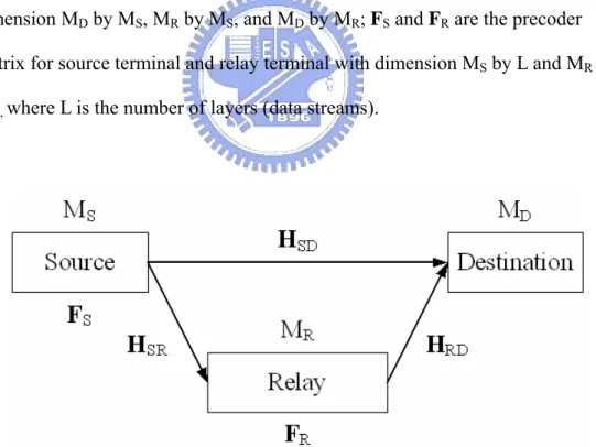
The system block diagram of a three-terminal MIMO relay system is depicted as in Figure 4.1 below. MS, MR, and MD represents the total antenna number of the corresponding terminal; the channel matrix between source and destination, source and relay, and relay and destination, are denoted as HSD, HSR, and HRD with

dimension MD by MS, MR by MS, and MD by MR; FS and FR are the precoder matrix for source terminal and relay terminal with dimension MS by L and MR by MR, where L is the number of layers (data streams).

(36)

4.2.2 Assumptions

Main assumptions are described as following:

1. In general, we don’t have any assumptions on the distribution of the channel matrices. But in numerical analysis, our channel matrices are modeled as block Rayleigh fading matrices with i.i.d. fading entries. 2. All channel matrices remain constant during one two-phase transmission.

The definition and details of two-phase transmission is the next section. 3. Channel matrices, noise vectors, and c, signal before source precoding,

are all mutually independent.

4. We assume that all channel matrices have full rank.

5. We assume that every terminal has perfect knowledge of all channels. 6. The relay operates in the half-duplex mode, which means that relay

cannot transmit and receive data simultaneously using same degree of freedom.

7. The relay neither decodes nor re-encodes the received signal. It only scales the received signal amplitude to fit its power constraint and

retransmits the modified signal to destination, i.e., it’s a non-regenerative (or amplify-and-forward, AF) relay.

8. We assume that the precoder input symbol vector c is a Gaussian input, which means that

(

D

)

CN 0,

c

∼

I

(37)

4.3 Two-phase Transmission Protocol

There are several variations that can be considered for two-phase

transmission protocols. The recently proposed cooperative diversity approaches demonstrate the potential to achieve higher diversity order or enhance the capacity of wireless systems without deploying multiple antennas at the transmitter. Using nearby collaborators as virtual antennas, significant diversity gains can be

achieved. These schemes basically require that the source terminal shares the information bits with the relay terminal(s), and this data sharing process is generally achieved at the cost of additional orthogonal channels

In the following slides the comparison of four common protocols, transmit diversity protocol, receive diversity protocol, simple transmit diversity protocol, and multihop protocol, will be presented. The discussions including:

z Transceiving relations among terminals. z Input-output relations between y and c. z Matrices A and B.

4.3.1 Transmit Diversity Protocol

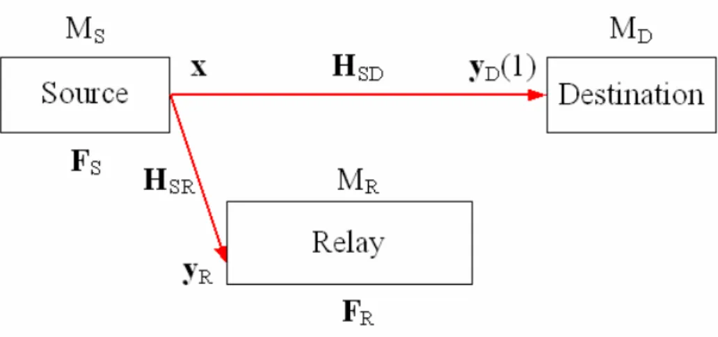
In the TD protocol, during the first phase, source terminal broadcasts its information. This process is depicted as in Figure 4.2(a). During the second phase, source terminal retransmits the same signal as in the first phase to destination terminal, and relay terminal transmits the precoded signal to destination terminal. This process is depicted as in Figure 4.2(b).

(38)

Fig. 4.2(a): The first phase of TD protocol

(39)

( )

(

( )

)

( )

R SR S R D SD S D D SD S RD R R D SD S RD R SR S R D SD S RD R SR S RD R R D D SD S D SD S RD R SR S RD 1 ( 1 1 1 (4 2 2 2 (4 2 1 2 2 1 2 1 1 2 2 1 = + − = + − = + + − = + + + = + + + ⎡ ⎤ ⎡ ⎤ =_⎢ _{⎥ ⎢}= _⎥ + + ⎣ ⎦ ⎣ ⎦ y H F c w y H F c w y H F c H F y w H F c H F H F c w w H F c H F H F c H F w w y H F 0 y c y H F H F H F H

( )

_{( )}

( )

R D R D R SD S D SD RD R SR S RD R D R SD S D SD RD R SR RD R D 1 2 2 1 1 2 1 ( 2 ⎡ ⎤ ⎡ ⎤ ⎢ ⎥ ⎢ ⎥ ⎢ ⎥ ⎣ _{⎦ ⎢} _⎥ ⎣ ⎦ ⎡ ⎤ ⎡ ⎤ ⎡ ⎤ ⎡ ⎤ ⎢ ⎥ =_⎢ _⎥_⎢ _⎥ +_⎢ _{⎥ ⎢} _⎥ ⎣ ⎦ ⎣ ⎦ ⎣ ⎦ _⎢ _⎥ ⎣ ⎦ ⎡ ⎤ ⎡ ⎤ ⎡ ⎤ ⎢ ⎥ =_⎢ _⎥ +_⎢ _{⎥ ⎢} _⎥ − ⎣ ⎦ ⎣ ⎦ _⎢ _⎥ ⎣ ⎦ x B A w I 0 w F 0 I w w 0 H F 0 I 0 c w H H F H F H F 0 I w w 0 H 0 I 0 F c w H H F H H F 0 I w 4 2) 3) 4) 4 5)

4.3.2 Receive Diversity Protocol

In this case, during the first phase, source terminal broadcasts its information in the same way as the TD protocol. This process is depicted in Figure 4.3(a). During the second phase, the relay retransmits the data to the destination terminal, and the source remains silent. This process is depicted in Figure 4.3(b).

(40)

Fig. 4.3(b): The second phase of RD protocol

( )

(

)

( )

_{( )}

( )

R SR S R D SD S D D RD R R D RD R SR S R D RD R SR S RD R R D R D SD S D D D RD R SR S RD R D SD RD R SR (4 6) 1 1 2 2 2 2 ( 1 1 2 2 = + − = + − = + = + + = + + ⎡ ⎤ ⎡ ⎤ ⎡ ⎤ ⎡ ⎤ ⎢ ⎥ =_⎢ _{⎥ ⎢}= _⎥ +_⎢ _{⎥ ⎢} _⎥ ⎣ ⎦ ⎣ ⎦ ⎣ ⎦ _⎢ _⎥ ⎣ ⎦ ⎡ ⎤ = ⎢ ⎥ ⎣ ⎦ A y H F c w y H F c w y H F y w H F H F c w w H F H F c H F w w w y H F 0 I 0 y c w y H F H F H F 0 I w H H F H

( )

R S D RD R D 1 ( 2 ⎡ ⎤ ⎡ ⎤ ⎢ ⎥ +_⎢ _{⎥ ⎢} _⎥ − ⎣ _{⎦ ⎢} _⎥ ⎣ ⎦ x B w 0 I 0 F c w H F 0 I w (4 7) 4 8)− 4 9)

4.3.3 Simple Transmit Diversity Protocol

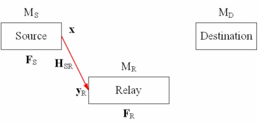
This is a simplified alternative approach to the TD protocol. In this case, the destination terminal is switched off during the first phase and thus ignores the signal from source terminal. The first phase communication link serves only the relay terminal. This process is depicted in Figure 4.4(a). The second phase is identical to that of the TD protocol. This process is depicted in Figure 4.4(b). The

(41)

STD protocol may result in a simple receiver structure but in some cases, a performance loss is expected compared to TD protocol.

Fig. 4.4(a): The first phase of STD protocol

(42)

( )

(

( )

)

( )

[

]

( )

_{( )}

[

]

[

]

[

]

R SR S R D SD S RD R R D SD S RD R SR S R D SD S RD R SR S RD R R D S R SD RD R SR RD R S D R SD RD R SR S RD R D 1 ( 2 2 1 2 1 2 1 (4 11) = + = + + = + + + = + + + ⎡ ⎤ ⎡ ⎤ = _⎢ _⎥ + _⎢ _⎥ ⎣ ⎦ ⎣ ⎦ ⎡ ⎤ = + _⎢ _⎥ ⎣ ⎦ A B y H F c w y H F c H F y w H F c H F H F c w w H F c H F H F c H F w w F w H H F H c H F I F w w H H F H F c H F I w 4 10)− −

4.3.4 Multihop Protocol

The effectiveness of MH protocols has been widely studied. This approach does not offer any diversity gain, and thus generally results in performance loss rather than gain. However, if the signal decay due to path loss is severe, the MH protocol does offer an SNR gain compared to direct transmission, when the relay is between the two communicating nodes. The process of MH protocol is depicted in Figure 4.5(a) and Figure 4.5(b).

(43)

Fig. 4.5(b): The second phase of MH protocol

(

)

(

)

[

]

R SR S R D RD R R D RD R SR S R D RD R SR S RD R R D R RD R SR S RD R D (4 12) (4 13) = + − = + = + + = + + ⎡ ⎤ = + _⎢ _⎥ ⎣ ⎦ A B y H F c w y H F y w H F H F c w w H F H F c H F w w w H F H F c H F I w −

4.3.5 Summary

A brief summary is depicted in Table 4.1:

TD RD STD MH T1 S→R S→D T1 S→R S→D T1 S→R T1 S→R Transceiving relation T2 S→R R→D T2 R→D T2 S→R R→D T2 R→D A SD SD RD R SR ⎡ ⎤ ⎢ ⎥ ⎣ ⎦ 0 H H H F H

[

HSD H F HRD R SR

]

⎡ SD ⎤ RD R SR ⎢ ⎥ ⎣ ⎦ H H F H H F HRD R SR B RD R ⎡ ⎤ ⎢ ⎥ ⎣ ⎦ 0 I 0 H F 0 I

[

H FRD R I

]

_{RD R} ⎡ ⎤ ⎢ ⎥ ⎣ ⎦ 0 I 0 H F 0 I

[

H FRD R I

]

(44)

4.4 Design Criterion: Ergodic capacity

In the previous chapter, we have formulated the input-output relation of various two-phase transmission protocols as a general form: a MIMO single link channel. For a MIMO single link channel with input-output relation

S

=

+

=

+

y

AF c Bw

Ax Bw

(4—14) the corresponding achievable rate of one two-phase transmission is given by [8] [19]:

(

)

1 H H H s S S W S

P

1 R

log det

2 M

−

⎛

⎞

=

_⎜

+

_⎟

⎝

I

AF F A

BR B

⎠

_(4—15)

where the factor 0.5 comes from the fact that the signal vector is actually

transmitted in two time instances, so the spectral efficiency drops by one half. PS is the source total transmit power, BRWBH is the equivalent noise covariance matrix,

A and B are functions of channel matrices, their form will depend on different

transmission protocol.

Based on equation (4-15), the ergodic capacity can be expressed as:

(

)

1 H H H s e S S S

P

1 C

E log det

2 M

−

⎧

⎛

⎞

⎫

⎪

=

_⎨

_⎜

+

_⎟

_⎬

⎪

⎝

⎠

⎪

⎩

I

AF F A

BR B

W

⎭

_(4—16)

where expectation operates on matrices A and B.

To maximize the average achievable rate, one can find optimal precoders that maximize the achievable rate per two-phase transmission, so the average of these maximum achievable rates will result in a maximum average achievable rate.

(45)

Without any constraint, maximization of ergodic capacity in (4—16) will lead to the trivial solution of increasing to the norm of precoder matrices to infinity. A reasonable constraint is obtained by bounding the expected norm of the transmit vector, which limit the transmit power. The individual power constraint for both precoder matrices are given by:

( )

{

H

}

{

(

H H

)

}

(

)

S S S S

E tr

= E tr

tr

H

P

S

=

≤

xx

F cc F

F F

(4—17)

(

)

{

}

(

)

{

}

(

)(

)

(

)

{

}

(

)

{

R

}

H R R H H R R R R H _H R SR S R SR S R R 2 H H H R w SR S S SR R R

E tr

= E tr

E tr

tr

σ

P

=

+

=

+

≤

x x

F y y F

F

H F c

w

H F c

w

F

I

H F F H

F

(4—18)

In summary, maximizing average achievable rate resulted in solving the following optimization problem:

(

)

(

)

(

)

₍ ₎

(

)

{

}

(

)

{

}

S R R 1 H H H s S R S S W S S,opt R,opt _, S R H S S S 2 H H H R w SR S S SR R R

P

,

log det

M

,

arg max

,

. . tr

P

tr

P

Q

s t

σ

−

⎛

⎞

=

_⎜

+

_⎟

⎝

⎠

=

≤

+

≤

F F

F F

I

AF F A

BR B

F

F F

F

I

H F F H

F

(4—19) where PS_{and P}R_{are the total transmit power transmitting a symbol vector by}

(46)

source and relay terminal.

4.5 Generic Algorithm Implementation

We can see from section 4.3.5 that matrices A and B share a common property: they not only are function of channel realization, but also function of relay precoder matrix.During each two-phase transmission, we have assumed that the channel realizations stay unchanged, which implies that under this condition, matrices A and B will be function of relay precoder matrix only.

Base on this observation, we can apply GA at relay terminal. First, generate a population of relay precoder matrix, say, 1000 relay precoder matrices, therefore, we can get 1000 matrices A and B.Base on [16] and [19], given a fix channel realization (matrices A and B) and full CSIT, the optimal source precoder matrix is to use water-filling strategy over all available subchannels. As a result, we can have 1000 precoder pairs for one channel realization.

Next step is to use these pairs to evaluate the block achievable rate. If we set crossover rate = 0.7, 300 best precoder pairs will be preserved, the remaining 700 precoders will be replaced by the offspring come from crossover. Here we use arithmetic crossover, where

Offspring = a*Parent1 + (1-a)*Parent2 + w (4—20)

with a = 0.5, and a small random zero-mean Gaussian matrix will be added on to tune it slightly. This random matrix can be considered as a secondary mutation

(47)

operation. When processing crossover, parents can be picked randomly from the “elites” or the “peasants”, where the probability being picked is proportional to its fitness value. Note that the factor a decides which side offspring is going to be like: if offspring is close to father, it will act like its father and share some common properties with its father; on the contrary, if offspring is close to mother, it will act like its mother and share some common properties with its mother;

After crossover operation, mutation operation steps in. The main mutation operation is a modified version of uniform mutation with a modified constraint such that every precoder matrix must follows the power constraint after any mutation operation. It is done simply by random generating another relay precoder matrix, force it to meet relay power constraint, and use this new precoder matrix to replace an old “peasant” matrix. The mutation rate is usually very small, say, 0.01. Only when the outcome of flipping a uniform dice is smaller than 0.01 will this mutation occurs.

Perform the whole process iteratively, say, 150 times for one channel realization, the final result will close to the optimal precoder pair. However, the GA parameters, including population size, crossover rate, mutation rate, and the iteration number needed for one channel realization, are highly related to the effectiveness of GA. Below we are going to use some simulations to find appropriate values of these parameters.

(48)

Convergence speed on GA parameters

Different GA parameters will affect GA’s convergence speed. The faster GA converges, the higher probability GA can find a better solution than the current solution. Through numerical analysis, the convergence speed of object function for different parameters will be showed. Nevertheless, by numerical analysis we will show that GA can find the optimal solution.

In numerical result 1, we are going to show the relationship between the convergence speed of the objective function and the GA population size. Parameter settings are listed below.

z Transmit protocol: RD

z All terminal antenna numbers: 2 z Number of layers: 2

z Crossover rate: 0.75 z Mutation rate: 0.05

z SNR0 = 10dB, SNR2 = 15dB, where SNR0 and SNR2 are defined as:

2 0 S S D 2 2 R R

SNR

P M σ

SNR

P M σ

=

_D _{(4—21) (4—22)}

(49)

Fig. 4.6: The convergence speed of objective function versus GA population size

In Figure 4.6, we can see that as the population size grows, the faster the convergence speed of the objective function. This is a reasonable result because that for one iteration the objective function value of the best candidate from a set with greater population size is higher than that from a set with smaller population size of high probability. However, increasing the population size does not always reduce the processing time, which implies that the resulting gain from increasing population vanishes as the population size grows to infinity.

Numerical result 2 shows the relationship between the crossover rate and the convergence speed of the objective function. Parameter settings are listed below.

(50)

z Number of layers: 2 z Population size: 500 z Mutation rate: 0.05

z SNR0 = 10dB, SNR2 = 15dB

Fig. 4.7: The convergence speed of objective function versus crossover rate

In Figure 4.7, we can see that when the crossover rate is too low, the convergence speed is comparatively slow because most candidates are kept as “elites” and offspring generated by crossover operation only contribute a very small part of this new population. Hence, crossover becomes ineffective and slows down the convergence speed. On the other hand, however, when the crossover rate is too high, the algorithm will easily falls into local optimum because the elite candidates lack gene variety. This problem will be even more severe if we only allow crossover between elite parents.

(51)

Numerical result 3 shows the relationship between the mutation rate and the convergence speed of the objective function. Parameter settings are listed below.

z Population size: 500 z Crossover rate: 0.75

z SNR0 = 10dB, SNR2 = 15dB

Fig. 4.8: The convergence speed of objective function versus mutation rate

In Figure 4.8, we can see that the relation between mutation rate and the objective function is not so obvious. However, if the mutation rate is too high, the algorithm will become a random search; if too low, the algorithm will lose the ability to climb out of the local optimum.

(52)

Numerical result 4 shows that GA actually approaches the optimal solution. This simulation considers no source precoder. Parameter settings are listed below.

z Transmit protocol: MH

z Population size: 1000 z Crossover rate: 0.7 z Mutation rate: 0.01 z SNR2 = 15dB

z Each SNR point averages over 1000 channel realizations.

Fig. 4.9: Comparison of ergodic capacity using different implementations

In Figure 4.9, we compare the ergodic capacity of four different

implementation schemes: blue line stands for the ergodic capacity that no relay precoder exists; green line comes from that we let relay precoder matrix of the

(53)

form: H RD SR R

=

F

V DU

(4—23) and we apply GA to find an optimal power loading matrix D; purple line

represents that we use GA to find a optimal relay precoder matrix; red line is the referenced algorithm in [4], where the relay precoder matrix is of the same form in (4—23) but with power loading matrix D = diag(f1,f2,…fMR) and

(

)

2 2 2 * 2

1

4

2

1

D k R k R k k R k R k

f

σ

ρ α

ρ α β μ

ρ α

σ

β

ρ α

+ R k

⎡

⎤

=

_⎣

+

−

_⎦

+

(4—24) where αks are the eigenvalues of HSRHSRHarranged in descending order, βks are the eigenvalues of HRDHHRD arranged in descending order, ρR is equal to

PS/(MS*σR2), and μ* is the unique Lagrange multiplier which satisfies the relay transmit power constraint.

From Figure 4.9, we can have two observations:

1. GA indeed reaches the optimal solution. The optimal relay precoder matrix proposed in [4] has already been proved to be optimal, and GA has the ability to find a solution that results a performance very close to the referenced algorithm in [4].

2. In the two-hop transmission protocol, relay precoder form as equation (4—23) has been proved an optimal form in [4]. This phenomenon can be confirmed by this numerical result because the green line and the purple line have almost same performance, which implies that the performance of directly selecting a optimal relay precoder matrix by GA is very close to that of selecting a optimal power loading matrix by GA

(54)

and then use equation (4—23) to form the relay precoder. Note that this observation can not be extended to other transmit protocols.

4.6 Summary

In this chapter, we have introduced the system model—three-terminal MIMO non-regenerative channel. Based on this model and the assumptions inposed on it, two-phase transmission protocols have been discussed; and then, we bring up a general input-output form for the equivalent channel resulted from these

two-phase transmission protocols. From this general form, we can therefore let the precoder pair design criteria—channel ergodic capacity, come into play. We also showed how we use GA to select the optimal precoder pair. In the end of this chapter, the relation between GA convergence speed and its parameters has been investigated, and the effectiveness of GA has been shown as well.

By using GA, we pick one optimal precoder pair for one transmission block; hence, the ergodic capacity can be maximized. In the next chapter, we will show some numerical results and observations.

(55)

Chapter 5 Numerical Result

In this chapter, we are going to show the numerical results. Four different transmission protocols will be examinated. Before we start, note that SNR0 is equal to PS/(MS*σD2), SNR1 is equal toPS/(MS*σR2), and SNR2 is equal toPR/(MR*σD2).

The numerical results have two parts: one is for ergodic capacity, and another is for outage capacity. We are going to find some insights from these results.

Part 1: Ergodic capacity

Analysis 1

Analysis 1 shows the comparison of the ergodic capacity of a three-terminal MIMO non-regenerative channel utilizing MH protocol. The analysis uses different implementation schemes while SNR2 has been set to 10dB and SNR1 varies from -10 to 40 dB. The numerical result is depicted in Figure 5.1, and the parameter settings are listed below:

z Transmit protocol: MH

z Population size: 500 z Crossover rate: 0.7 z Mutation rate: 0.01 z SNR2 = 10dB.

(56)

Fig. 5.1: Numerical result 1

In Figure 5.1, blue line stands for the ergodic capacity that neither source nor source relay precoder exists; green line represents algorithm 1 from reference [4] which has been explained in detail in section 4.5; purple line is the performance for the optimal precoder pair discovered by GA; red line is from reference [9], which considers both source precoder and relay precoder matrices. Reference [9] uses singular value decomposition (SVD) to transform the two-hop MIMO channel into parallel Gaussian channels, and the source precoder matrix and relay precoder matrix are set to match the parallel channels with the form:

S SR S H R RD R S

=

F

V D

F

V D U

_R (5—1)(5—2)

(57)

R,m m m S,m m R,m m S,m m _m R,m m S,m m

P b

4a

1 P

1 a

2 P b ν

P a

4b

1 P

1 b

2 P a ν

+ +

⎡

⎛

⎞

⎤

=

⎢

⎜

_⎜

+

−

⎟

_⎟

⎥

⎢

_⎝

_⎠

⎥

⎣

⎦

⎡

⎛

⎞

⎤

=

⎢

⎜

_⎜

+

−

⎟

_⎟

⎥

⎢

_⎝

⎥

⎣

⎦

1

1 −

−

⎠

_{(5—3) (5—4)}

where ν is the Lagrange multiplier chosen to satisfy the individual power

constraint for source and relay terminal. Reference [9] also considers subchannel pairing such that the in a two-hop MIMO channel, subchannelsof both hops are paired together according to their actual magnitude. In our simulation we let all available subchannels be paired together as in [9]. Also note that [9] does not claim its result an optimal solution.

By comparing the green and red lines, we can see clearly that an additional source precoder does enhance the performance in low SNR region. The performance gain vanishes as the SNR grows higher. This makes sense since when SNR is low, source precoder will prevent the transmit power to be load onto null subchannels or subchannels with bad condition. However, when the SNR is high, the

water-filling strategy suggests that load the power equally onto all available subchannels, which is the same as if there is no source precoder. Also note that the GA-optimal precoder pair results a small performance gain over referenced

algorithm 2 in the low SNR region, the performance gain over algorithm 2 decreases as SNR increases as well.

Analysis 2

(58)

MIMO non-regenerative channel utilizing RD protocol. The analysis uses different implementation schemes while SNR0 and SNR2 have been set to 10dB and SNR1 varies from -30 to 40 dB. The numerical result is depicted in Figure 5.2, and the parameter settings are listed below:

z Population size: 500 z Crossover rate: 0.7 z Mutation rate: 0.01 z SNR0 = SNR2 = 10dB.

(59)

Figure 5.2 contains three lines: blue line represents performance without precoder pair; the purple line is system ergodic capacity with GA-optimal relay precoder only; green line is system ergodic capacity with GA-optimal precoder pair.

Like the MH protocol case, adding a source precoder has a performance gain in low SNR region, but this gain vanishes as SNR approaches infinity.

Performance gain in high SNR region comes from the fact that in RD protocol the receiver use maximum-ratio combining (MRC) to detect signal, so when SNR1 raises, the signal of relay-destination link becomes more reliable and hence boosts the performance.

Analysis 3

Analysis 3 shows another comparison of ergodic capacity of a three-terminal MIMO non-regenerative channel utilizing RD protocol. The Analysis uses

different implementation schemes while SNR0 has been set to -10 dB, SNR2 has been set to 10dB and SNR1 varies from -30 to 40 dB. The numerical result is depicted in Figure 5.3, and the parameter settings are listed below:

z Population size: 500 z Crossover rate: 0.7 z Mutation rate: 0.01

(60)

Analysis 4

Analysis 4 shows another comparison of ergodic capacity of a three-terminal MIMO non-regenerative channel utilizing RD protocol. The Analysis uses

different implementation schemes while SNR0 and SNR2 have been set to -10dB and SNR1 varies from -30 to 40 dB. The numerical result is depicted in Figure 5.3, and the parameter settings are listed below:

(61)

z Crossover rate: 0.7 z Mutation rate: 0.01 z SNR0 = SNR2 = -10dB.

Analysis 5

Analysis 5 shows the comparison of ergodic capacity of a three-terminal MIMO non-regenerative channel utilizing STD protocol. The analysis uses different implementation schemes while SNR2 has been set to 10dB and SNR1 varies from -30 to 40 dB. The numerical result is depicted in Figure 5.5, and the parameter settings are listed below:

z Transmit protocol: STD

(62)

z Number of layers: 2 z Population size: 500 z Crossover rate: 0.7 z Mutation rate: 0.01 z SNR2 = 10dB.

In figure 5.5, there are three lines. The blue line represents performance without precoder pair; the purple line is system ergodic capacity with GA-optimal relay precoder only; green line is system ergodic capacity with GA-optimal precoder pair. As expected, system with an additional source precoder always performs better than system without source precoder in low SNR region.

以基因演算法研究三點式非再生性MIMO中繼站系統之最佳Precoder Pair

國 立 交 通 大 學

電信工程學系碩士班

碩 士 論 文