使用卡曼濾波器追蹤參考訊號之適應性語音純化波束形成器

國 立 交 通 大 學

電機與控制工程研究所

碩 士 論 文

使用卡曼濾波器追蹤參考訊號之

適應性語音純化波束形成器

Adaptive Beamformer for Speech Enhancement

Using Kalman Filter with Reference Signal Tracking

研 究 生： 朱 育 成

指導教授： 胡 竹 生 博士

使用卡曼濾波器追蹤參考訊號之

適應性語音純化波束形成器

Adaptive Beamformer for Speech Enhancement

Using Kalman Filter with Reference Signal Tracking

研 究 生：朱 育 成

Student: Yu-Cheng Chu

指導教授：胡 竹 生 博士

Advisor: Dr. Jwu-Sheng Hu

國立交通大學

電機與控制工程學系

碩 士 論 文

A Thesis

Submitted to Institute of Electrical and Control Engineering College of Electrical Engineering

National Chiao Tung University in partial Fulfillment of the Requirements

for the Degree of Master in

Electrical and Control Engineering September 2011

Hsinchu, Taiwan, Republic of China

使用卡曼濾波器追蹤參考訊號之

適應性語音純化波束形成器

研究生：朱 育 成 指導教授：胡 竹 生 博士 國立交通大學電機與控制工程研究所碩士班

摘 要

本論文提出一套利用麥克風陣列來降低噪音及迴響效應的演算法。在實際環 境中，目標音訊不只常受到穩態雜訊及非穩態雜訊的干擾，更常因為迴響效應而 使語音品質遭到破壞。因此，本論文期望設計一個能濾除雜訊並減少迴響影響的 適應性波束形成器。此演算法在波束形成器演算法中，引入參考訊號的觀念並輔 以 Kalman 濾波器來進行演算。此外，經過些微的修改，本演算法也可以利用於 偵測語音活動。藉由適當的語音活動偵測，可以幫助分辨目標與噪音在本質上的 不同，並且加速 Kalman 濾波器的收斂。利用實際在車上錄得的音檔進行的實驗 結果也在此篇論文中呈現。本論文並利用客觀的參數評估所提出的波束形成器與 語音活動偵測的效能，並與其他已知的方法進行比較分析。

Adaptive Beamformer for Speech Enhancement

Using Kalman Filter with Reference Signal Tracking

Student：Yu-Cheng Chu Advisor：Dr. Jwu-Sheng Hu

Institute of Electrical and Control Engineering

A

BSTRACT

In this thesis, an algorithm that considers noise reduction and de-reverberation simultaneously using microphone array is proposed. In many practical environments, the desired speech signal is usually contaminated by stationary or non-stationary noises and distorted by reverberation. When considering noise reduction only, the desired speech signal could be distorted further due to the effect of desire signal cancellation etc. The objective of this thesis is to design an adaptive beamformer to incorporate de-reverberation into the noise reduction framework. The proposed method tracks a pre-recorded reference signal to compensate the reverberation effect. Consequently, the algorithm results in a trade-off between the two objectives. Further, a voice activity detection (VAD) algorithm is proposed by slightly modifying the proposed algorithm. An adequate VAD can help to identify the nature of signal and noise and accelerate the convergence rate of Kalman filter. The experiments on real car sound samples are processed. The performance of beamformer and voice activity detection are both evaluated and compared with existing algorithms.

致謝

這篇論文的完成，首先感謝我的指導教授胡竹生教授。他給予我許多栽培及 建議、討論，讓我在思索、研究的過程中更能瞭解科學研究的精神，讓我收益良 多。接著感謝我的父親朱榮洲以及母親陳秀珍，在這兩年的求學過程中，讓我可 以無後顧之憂的完成學位，而父母親在心靈上以及感情上的支持，更是無時無刻 支持我走下去的動力。有太多時候我都很挫折、很沮喪，但是只要聽到爸媽的聲 音、想起你們的殷切盼望以及無私的栽培，我就又能鼓起勇氣繼續向前。 在兩年的過程中，X-Lab 實驗室就像我的第二個家，在這裡有許多共同求學 的同學們以及親切又知識淵博的學長們。最先感謝的是李明唐學長，這兩年來， 每次與他討論的過程總讓我進步許多，他給的建議也都能發揮莫大的助益，對學 長的感激溢於言表。而已經畢業的楊佳興學長，在我研究的過程中，給我許多的 文件，讓我等於直接吸收了他多年的功力，讓我的見識又更上一層。另外，溫柔 而親切的永融學長、熱心也很有想法的阿吉學長、有趣但是運氣一直不太好的崇 維學長、威武聰明但不失幽默的冠群學長、溫和愛運動的智謙學長、開朗陽光的 庭昭學長，諸位學長們在我求學的過程中都讓育成的人生增添了許多的色彩與長 進。另外一位不得不提的則是鎮宇學長，能進入 X-Lab 就先要感謝他兩三年前的 建議。在實驗室的最後一年，能和鎮宇學長一起在實驗室做研究、到處吃喝、打 球，甚至是傾吐心事，都讓我的碩二過得快樂許多。實驗室的同學們，感謝很 high 點子很多的湘筑、有活力有想法的偉庭、見解獨到很能幫助討論的建安、很健談 幽默的新文、不健談但很幽默的昀軒、很健談但不幽默的學文，這兩年來有各位 的陪伴，真是育成的榮幸。學弟們，很嘴砲很開朗的昭男、顯圖很閃的耕維、做 事認真的哲鳴以及一樣有趣的建廷宗翰，這些日子以來感謝你們。 電資 98 的各位，各位的陪伴與支持也不可或缺。嘴砲的雄獅一哥宗憲、在國 外努力生活的紹甫、一起打 BG 打球的紹丞、很嘴砲也很風趣的育瑞、就在對面 很常遇到可以分享垃圾事聊天的冠甫、奕奇，這六年有你們真好！ 謝謝交通大學這六年來的栽培，這絕對是我人生中精彩的旅程！

C

ONTENT

摘 要 ... i ABSTRACT ... ii 致謝 ...iii CONTENT ... iv LIST OF TABLES ... vi

LIST OF FIGURES... vii

Chapter 1. INTRODUCTION... 1

1.1 Motivation and Objective ...1

1.2 Literature Review ...2

1.3 Thesis Subject and Contribution...4

1.4 Outlines of Thesis ...4

Chapter 2. BEAMFORMER USING KALMAN FILTER ... 6

2.1 Introduction...6

2.2 Beamformer under MVDR Structure ...6

2.3 Beamformer Using Kalman Filter under MVDR Structure ...8

Chapter 3. REFERENCE-SIGNAL-BASED BEAMFORMER... 11

3.1 Introduction...11

3.2 Formulation of Referenced-Signal-Based Beamformer Using Kalman Filter ...11

3.3 Solution to the Proposed Formulation ...13

3.4 Parameter Selection and Tradeoff...17

3.5 Voice Activity Detection under Proposed Formulation ...19

3.6 Threshold Decision and SINR Estimation...22

3.6.1 Gaussian Mixture Model and EM Algorithm...22

3.6.2 SINR Estimation...27

3.7 Overall System Architecture...29

Chapter 4. EXPERIMENT RESULTS... 33

4.2 Experiments on Performance of Noise Reduction and Its Tradeoff with

Dereverberation ...36

4.3 Performance on Voice Activity Detection ...42

Chapter 5. CONCLUSION AND FUTURE STUDY ... 50

L

IST

O

F

T

ABLES

TABLE 1COMMON PARAMETERS IN EXPERIMENT...33

L

IST

O

F

F

IGURES

FIG.1BLOCK DIAGRAM OF THE CONSTRAINED KALMAN ALGORITHM WITHOUT PRIOR

ESTIMATION OF THE DESIRED SIGNAL...10

FIG.2FLOW CHART OF VOICE ACTIVITY DETECTION PROCEDURE...21

FIG.3SCHEMATIC ILLUSTRATION OF ERROR DISTRIBUTION:(A)DISTRIBUTION OF NOISY SPEECH;(B)DISTRIBUTIONS OF SPEECH AND NONSPEECH (THIS FIGURE IS MODIFIED FROM [9]) ...23

FIG.4EM ALGORITHM WITH CONSTRAINTS (REVISED FROM [9]) ...1

FIG.5THE PROCESS OF VAD DECISION (REVISED FROM [9]) ...1

FIG.6THE RELATIONSHIP FROM MEAN DIFFERENCE IN VAD TO THE BEST ESTIMATION OF  ...27 _v FIG.7AN EXAMPLE OF TRAINED RELATIONSHIP FROM SINR TO MEAN DIFFERENCE....28

FIG.8SINR VS. THE _v GIVING BEST LSD ...29

FIG.9THE FLOWCHART OF OVERALL SYSTEM...31

FIG.10THE PHOTO FOR THE MICROPHONE ARRAY AT THE SUN SHIELD OF THE DRIVER’S SEAT. ...34

FIG.11THE PHOTO FOR THE HATS AT THE DRIVER’S SEAT...34

FIG.12EXPERIMENT RESULTS IN CAR ENVIRONMENT WITH INPUT SNR7 DB ...38

FIG.13EXPERIMENT RESULTS IN CAR ENVIRONMENT WITH INPUT SNR2 DB ...38

FIG.14EXPERIMENT RESULTS IN CAR ENVIRONMENT WITH INPUT SNR-4 DB...38

FIG.15EXPERIMENT RESULTS IN CAR ENVIRONMENT WITH INPUT SINR7 DB...39

FIG.16EXPERIMENT RESULTS IN CAR ENVIRONMENT WITH INPUT SINR2 DB...40

FIG.17EXPERIMENT RESULTS IN CAR ENVIRONMENT WITH INPUT SINR-4 DB ...41

FIG.18VOICE ACTIVITY DETECTION UNDER SINR=10 DB ...45

FIG.19VOICE ACTIVITY DETECTION UNDER SINR=5 DB ...46

FIG.20VOICE ACTIVITY DETECTION UNDER SINR=0 DB ...47

FIG.21VOICE ACTIVITY DETECTION UNDER SINR=-5 DB ...48

Chapter 1. I

NTRODUCTION

1.1 Motivation and Objective

Our hearing is perhaps the the most useful sense except vision. However, the information retrieved from hearing is usually contaminated by undesired sources. Although human beings are able to recognize desired speeches under interferences, it is still considered as a difficult task for computers or machines.

A common sensor for receiving sound wave is the microphone. Single microphone can collect spectral information but not spatial information. To retrieve more information among the sound wave, a collection of microphones, or microphone array, is applied to catch not only spectral information but also spatial information. Among several existing microphone-array-based enhancement algorithms, beamformer is one of the most popular methods and was extensively studied for hands-free speech communication or recognition.

Background noise and reverberation are the most common origin to signal quality degradation. The background noise is from undesired noise source or interferences. The spectral and spatial likelihood between noise and desired source will determine the difficulty of removing noise. The reverberation level will determine the distortion to the desired source. The reverberation level is commonly affected by the reflection ratio and openness of the environment.

The purpose of the thesis is to design a beamformer that handles both noise reduction and dereverberation. A scenario like car environment is possible to occur in real life, where the quality of sound is seriously deteriorated by engine noise and wind

noise and reverberation from the narrow space of cabin.

1.2 Literature Review

The beamformers can be categorized in two types, fix beamformers and adaptive beamformers. Most of the fix beamformers are simpler than the adaptive beamformers. The implementation costs of fix beamformers are often lower than the adaptive

counterparts.

Fix beamformers includes delay-and-sum beamformer (DSB) [11], constant directivity beamformer (CDB) [12] and fixed superdirective beamformers [13]. They utilize fixed coefficients to achieve a desired spatial response. The DSB is the simplest structure in fix beamformers. It first compensates to the relative time delay between distinct microphone signals and then sums the steered signal to form a single output. CDB is designed to maintain the spatial response equal over a wide frequency band while the fixed superdirective beamformer attempts to suppress noise coming from all directions without affecting the desired speech signal from a principal direction. Fix beamformers generally assume the desired sound source, interference signals, and noises are slowly varying and at known locations. Therefore, these algorithms are sensitive to steering errors, which limit their noise suppression capability and give rise to the desired signal distortion and cancellation. Furthermore, these algorithms also have limited performance under highly reverberation environments.

Instead of using fixed coefficients to suppress noises and interference signals, an adaptive beamformer can form its directivity beam-pattern to the desired signal and its null beam-pattern to the undesired signals. In the fixed beamformers, the beam-pattern

of null only exists when the direction of noise is known and remains unchanged. To cope with environmental changes, various adaptive beamformers were proposed to improve the performance. One key issue in adaptive beamformers is the sensitivity due to the mismatch between the actual desired signal steering vector and the presumed one [10]. The mismatch can be induced by signal pointing errors [14], imperfect array calibration [15], or channel effect. In the presence of these effects, an adaptive

beamformer can easily mix up the desired signal and interference components; that is, it suppress the desired signal instead of maintaining distortionless response. This phenomenon is commonly referred to signal self-nulling [16]. As a result, much effort has been devoted to the noise reduction and dereverberation.

Many adaptive beamformer techniques were extensively studied. The linearly constrained minimum variance (LCMV) beamformer was proposed in [17] to

minimize the array output power under a look direction constraint. A form similar to LCMV is minimum variance distortionless response (MVDR) proposed by Capon in [1]. Another popular technique is the generalized sidelobe canceller (GSC) algorithm which essentially transforms the LCMV constrained minimization problem into an unconstrained one [18].

The formulation of MVDR is then revisited in [5] with Kalman filter by introducing the concept of state space. To improve the robustness against steering vector error, various methods are investigated [10]. The Kalman filter can be also substituted by H-infinity filter or Second Order Kalman filter or Second Order H-infinity filter [19] to enhance its robustness and reducing non-linearity.

solve channel effect. The algorithm by Dahl et. al can be found in [20], which give rise to the reference signal concept in proposed algorithm.

1.3 Thesis Subject and Contribution

The contribution of this thesis is to propose and implement an innovative algorithm for speech enhancement. The subject of this thesis can be divided into two parts. The first part is to formulate a new beamformer considering given the information of pre-recorded data. The solution to the formulation is presented. The second part is to handle the resulting voice activity detection problem by the same formulation but only changes the parameters to render different results.

In the first part, the formulation using MVDR with pre-recorded signal is given. To solve the formulation, the linear first order Kalman filter is used. In the Kalman filter, the selection of parameters will pose different result among noise reduction and dereverberation. The tradeoff effect is discussed and explained.

In the second part, the same formulation is used to implement a voice activity detector. The design and parameter choosing technique are explained and discussed. Besides, the information given by the voice activity detector can be reused to finding the appropriate parameter in beamforming.

The experiment results are shown to verify the performance of the proposed algorithm, both in beamforming and voice activity detection.

1.4 Outlines of Thesis

Chapter 2: The basic beamforming technique Minimum Variance Distortionless Response (MVDR) is introduced. The optimal solution of MVDR is

presented. The method of incorporating state space formulation into solving MVDR and solve it with Kalman filter is investigated. These constructed the foundation of proposed algorithm.

Chapter 3: The detailed concept of reference signal based Kalman filter for

beamformer is stated. It includes the beamforming formulation and voice activity detection. In beamforming, the formulation and its solution are presented. The technique of choosing the parameter and its effect are also discussed. In voice activity detection (VAD), the design and implementation are investigated. The method of utilizing the information from VAD to decide the parameters in beamforming is also described. Finally, the overall architecture is illustrated and explained.

Chapter 4: The experiment results are presented. It contains experiments regarding beamforming capability and voice activity detection. Some objective indices are calculated to compare the performance of proposed algorithm and former algorithms.

Chapter 5: The conclusion of this thesis and some issue that is still not clear is discussed is this chapter.

Chapter 2.

B

EAMFORMER

U

SING

K

ALMAN

F

ILTER

2.1 Introduction

Kalman filter is a well-known optimal estimation filter in control theory. In this thesis, the use of Kalman filter in signal processing is more concerned. To begin with, a conventional beamformer MVDR proposed by Capon [1] is introduced. The main idea of MVDR is to minimize undesired noise while maintaining desired signal with known DOA, or Direction of Arrival, distortionless. Such idea can be formulated as a minimization problem with certain constraints. Conventional way to solve it is using Lagrange Multiplier and achieves optimal solution. Its optimal solution is presented in Section 2.2. In Section 2.3, the technique of incorporating state space concept and Kalman filter to solve MVDR problem is presented. The solution can be found using conventional Kalman filter solution. In later sections, another formulation to maintain the distortionless constraint will be presented and investigated.

2.2 Beamformer under MVDR Structure

The minimum variance distortionless response (MVDR) beamformer, also known as Capon beamformer [1], minimizes the output power of the beamformer under a single linear constraint on the response of the array towards the desired signal.

Consider the conventional signal model in which an M-element microphone array captures a convolved desired signal (speech source) in some noise field. The received signals are expressed as [2], [3], [4]

1,2,...M m ) ( ) ( * ) (k a s k v k  x_{m m m} , (2.1)

where is the impulse response from the unknown (desired) source to the microphone, * stands for convolution, and is the noise at the microphone . The signals and are assumed as uncorrelated and zero mean.

m a s(k) th m m ) (k vm ) (k s vm(k)

In the frequency domain, (2.1) can be written as

1,2,...M m ) ( ) ( * ) ( ) (jw  A jw S jw V jw  X_{m m m} , (2.2)

where , , , are the discrete-time Fourier transforms

(DTFTs) of , , , , respectively, at angular frequency ) ( jw Am a_m ) ) ( jw S ) k s(k ) ( jw Xm ) (k x_m ) ( jw Vm ) (k v_m ( ) (   w

w and j is the imaginary unit ( j2 1).

These M microphone signals in the frequency domain are summarized in a vector notation as ) ( ) ( ) ( ) (jw A jw S jw V jw X   , (2.3) where T M M T M (jw) V (jw) (jw) V V jw (jw) A (jw) (jw) A A (jw) jw X jw X jw X jw ] [ ) ( ] [ )] ( ) ( ) ( [ ) ( 2 1 T 2 1 2 1       V A X

and superscript denotes transpose of a vector or a matrix. T

Consider finding a weight vector which satisfies the look direction constraint MV w 1 ) , ( ) (jw _s jw  H MV a w (2.4) while attempting to minimize beamformer output power

) ( ) ( ) ( } ) ( ) ( { } ) ( {Y jw 2 E jw jw 2 jw jw jw E  wH_MV X w_MVH R_XX w_MV (2.5)

beamformer output given by ) ( jw Y =wH_MV( jw) X( jw). (2.6) ) , (_s jw

a is the array manifold vector that points to the source direction.

With the consideration above, the following constrained optimization problem can be formulated: 1 ) , ( ) ( subject to ) ( ) ( ) ( min jw jw jw jw s jw  H MV MV XX H MV R w w a  w (2.7)

To solve this problem, the Lagrange Multiplier is incorporated.

         1 ) , ( ) ( 0 ] 1 ) , ( ) ( [ ) ( ) ( ) ( ( ) ) ( jw jw jw jw jw jw jw s H MV s H MV jw W MV XX H MV jw W_{MV MV}    a w a w w R w (2.8) (2.8) can be reduced to      1 ) , ( ) ( ) , ( ) ( ) ( jw jw jw jw jw s H MV s MV XX    a w a w R (2.9)

Assuming RXX is nonsingular. Then

, ) , ( ) ( ) , ( ) , ( ) ( ) ( ₁ 1 jw jw jw jw jw jw s XX s H s XX MV _{ }  a R a a R w _   (2.10)

which is the optimal solution to MVDR problem proposed by Capon[3] and is thoroughly evaluated in [4].

2.3

Beamformer Using Kalman Filter under MVDR Structure

The traditional formulation and solution to MVDR is presented in Section 2.2. In this section, The Kalman filter is introduced to solve the MVDR problem in a new formulation by Y.H. Chen and C.T. Chiang [5].

With the same formulation as (2.7), the two equations are written in model measurement equation as

) , ( ) , ( ) , ( or ) , ( ) , ( ) , ( ) , ( ) , ( 1 0 2 1 jw k jw k jw k jw k v jw k v jw k jw jw k H s H H V w B Y w a X                        , (2.8)

where T, and the input vector is given by ] 1 0 [  Y        ) , ( ) , ( ) , ( jw jw k jw k s H H H  a X B (2.9) and the measurement noise vector is

       ) , ( ) , ( ) , ( 2 1 jw k v jw k v jw k V . (2.10) Here, is the residual error and is the constraint error. By the

assumption that and are uncorrelated, the correlation matrix of can be written as ) , ( 1 k jw v ) jw ) , ( 2 k jw v ) , ( 1 k jw v v₂(k, jw) , (k V          ₂ 2 2 1 0 0 v v Q   (2.11)

Since the optimum-constrained weight vector is a constant all the time for the stationary environment [6], the truth-model process equation of the constrained Kalman algorithm may be written as

) , (k jw w ). , 1 ( ) , (k jw  w k jw w (2.12)

With the process equation (2.12) and measurement equation (2.8), the constrained Kalman algorithm can minimize the residual error in the mean-square sense while maintaining a distortionless response along the look direction.

After applying the discrete Kalman filter theory with (2.12) and (2.8), the filtered estimate of the weight vector is recursively given by [6]

)], , 1 ( ˆ ) , ( ) , ( )[ , ( ) , 1 ( ˆ ) , ( ˆ k jw w k jw K k jw Y k jw BH k jw w k jw w (2.13)

. ] ) , ( ) , 1 ( ) , ( )[ , ( ) , 1 ( ) , (k jw  k jw k jw k jw ee k jw k jw Q 1 H ee B B R B R K (2.14)

Here the filtered weight-error correlation matrix R_ee(k,jw) is ), , 1 ( )] , ( ) , ( [ ) , (k jw k jw H k jw _ee k jw ee  IK B R  R (2.15)

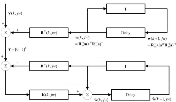
where is an identity matrix. Using (2.8), (2.12), (2.13), the signal-flow graph of the constrained Kalman algorithm can be plotted as Fig. 1 [5].

I m-by-m

Fig. 1 Block diagram of the constrained Kalman algorithm without prior estimation of the desired signal

Chapter 3. R

EFERENCE-

S

IGNAL-

B

ASED

B

EAMFORMER

3.1 Introduction

The MVDR structure can be modified by exploiting the distortionless response. To maintain desired signal distortionless, the algorithm incorporating pre-recorded signal as reference signal is proposed. The reference signal enhances the distortionless constraint by using more information and reduces the loading of carefully estimating the system parameters of the environment. More detailed explanation will be presented in this chapter.

In this chapter, the main algorithm of using reference signal to merge with MVDR and Kalman filter is presented. In Section 3.2, the formulation under that concept is proposed and described. In Section 3.3, the solution to solving proposed formulation is thoroughly investigated. In Section 3.4, the know-how of how to choose the parameters of the Kalman filter is discussed. The tradeoff phenomenon between the parameters is introduced and explained also in Section 3.4. The design and implementation of voice activity detection elaborating the same Kalman filter is presented in Section 3.5. The threshold decision method and parameter selection method is introduced in Section 3.6. The overall system architecture is illustrated and explained in Section 3.7.

3.2 Formulation of Referenced-Signal-Based Beamformer Using

Kalman Filter

filter is presented.

In MVDR beamformer, the distortionless requirement is achieved by add a constraint that maintains the signal from a known direction unchanged. This constraint also avoids choosing the naïve solution of zero during the minimization process. In addition, this constraint also achieves the requirement of dereverberation since it not only preserves signal from desired direction, but also drop reverberation signals from other directions during the minimization process.

Another approach to maintain distortionless requirement is to estimate the acoustic transfer function (ATF) from the desired signal source to the microphone array. The ATFs can specifically describe the relationship from desired source to the microphone array including the effect of reverberation. With the ATFs, source signal can be regenerated with low distortion as long as the ATFs are estimated correctly and the surrounding environment is linearly time-invariant (LTI) and does not change during the filtering process.

However, estimating the ATFs is a cumbersome and tedious work. To avoid such process but still get useful knowledge of the environment, the concept of reference-signal is incorporated. The reference-signal is acquired by recording the signal while playing a known clip at the position of source. The received signal can be considered as the output of the known input processed by the surrounding environment functioned as the system. With the input and output information of the system, it can be considered as a reference to the environment and thus achieving the requirement of distortionless better and easier.

. 1 ) , ( ) ( subject to ) ( ) ( ) ( min jw jw jw jw s w  H MV MV XX H MV R w w a w (2.7)

To incorporate the reference-signal, the formulation can be used to substitute the distortionless constraint and becomes

), ( ) ( ) ( subject to ) ( ) ( ) ( min jw s jw jw jw jw jw r r H MV MV XX H MV  X w w R w (3.1)

where is the discrete-time Fourier transforms (DTFTs) of the played known clip and is discrete-time Fourier transforms (DTFTs) of the received signal

while playing the known clip. , where is the

discrete-time Fourier transforms (DTFTs) of received signal at the microphone. The subscript “r” implies “pre-recorded” since the reference signal is recorded before

the filtering process.

) ( jw s_r ( r X jw) T M r r r r(jw)[X ,1 X ,2  X , ] X Xr,m th m

3.3 Solution to the Proposed Formulation

With the formulation above,

), ( ) ( ) ( subject to ) ( ) ( ) ( min jw s jw jw jw jw jw r r H MV MV XX H MV  X w w R w (3.1)

the solution to the formulation will be presented in this section [2].

From (3.1), state equations describing such formulation can be written as Measurement Equation: ) , ( ) , ( ) , ( ) , ( ) , ( 0 w k w k w k w k w k s H r H r V w X X               (3.2) Process Equation: ), , ( ) , ( ) , 1 (k w w k w Q k w w    (3.3)

where is the frame index and the superscript “H

” means conjugate-transpose. The noise and are assumed with Gaussian distribution and thus the covariance matrix can be written as

k ( V k, w) Q(k,w) ), 0 0 1 , 0 ( ~ ) , ( ) , 0 ( ~ ) , (       v v Q N w k I N w k    V Q (3.4)

where “N” means Normal Distribution and  , Q  , v  are parameter to be chosen. v is the received signal when desired signal is inactive, since the desired signal cannot always be guaranteed uncorrelated with the reference-signal. Once desired signal is correlated with reference signal, the phenomenon “desired signal cancelation” will occur and yield huge degradation to the desired signal.

) , (k w

X

Let the state estimation error is

), , 1 ( ˆ ) , ( ) , 1 (kk w w k w w kk w e (3.5) and the error covariance matrix is

)] , 1 ( ) , 1 ( [ ) , 1 (kk w E kk w T kk w ee   e  e  R (3.6) In the first step, no new observation is used. To predict using the state equation, the best possible predictor given no new information is available would be

) (k w ). , 1 1 ( ˆ ) , 1 ( ˆ kk w w k k w w (3.7) The estimation error is

) , ( ) , 1 1 ( ) , 1 1 ( ˆ ) , ( ) , 1 ( ) , 1 ( ˆ ) , ( ) , 1 ( w k w k k w k k w k w k w k k w k w k k Q e w Q w w w e               　　　　 　　　　 (3.8)

constant bias in the optimal linear estimation [7]), E e[ (kk w1, )]0. Since ) , 1 1 (k k w e is uncorrelated with Q(k,w), ) , 1 (kk w ee  R =R_ee(k1k1 w, ) ) , (k w Y . 2 I Q (3.9) This is the Riccati Equation.

In the second step, the new observation, = is incorporated to

estimate . A linear estimate that is based on

      ) , ( 0 w k sr ) , (k w

w wˆ(kk1 w, ) and has the

form ) , (k w Y (3.10) ), , ( ) , ( ( ˆ ) , ( ' ) , ( ˆ kk w K k w w k k w Y k w w  kk1 w, )

where and are some matrix and vector to be determined. The vector is called the Kalman gain. Now, the estimation error is

) , ( ' k w K k(k,w) ) , (k w k ), , ( ) , ( ) , 1 ( ) , ( ' ) , ( ] ) , ( ) , ( ' [ )] , ( ) , ( ) , ( )[ , ( )] , 1 ( ) , ( )[ , ( ' ) , ( ) , ( ) , ( ) , 1 ( ˆ ) , ( ' ) , ( ) , ( ˆ ) , ( ) , ( w k w k w k k w k w k w k w k w k w k w k w k w k k w k w k w k w k w k w k k w k w k w k k w k w k k H H V k e K w k K I V w k e w K w Y k w K w w w e                   X X 　　　　 　　　　 　　　　 (3.11) where _.       ) , ( ) , ( ) , ( w k w k w k _H r H H X X X

Since E e[ (kk w1, )]0, then E e[ (kk,w)]0 only if H w k w k, ) ( , )X ( ' I k K   (3.12) With this constraint, it follows that

)], , 1 ( ˆ ) , ( )[ , ( ) , 1 ( ˆ ) , ( ) , ( ) , 1 ( ˆ ] ) , ( [ ) , ( ˆ w k k w k w k w k k w k w k w k k w k w k k H H          w Y k w Y k w k I w X X 　　　　 (3.13) and

). , ( ) , ( ) , 1 ( ] ) , ( [ ) , ( ) , ( ) , 1 ( ) , ( ' ) , ( w k w k w k k w k w k w k w k k w k w k k H V k e k I V k e K e        X 　　　　 (3.14)

Since V(k,w) is uncorrelated with Q( wk, ) and with Y(k1,w), then V(k,w) will be uncorrelated with w(k,w) and with wˆ k( k1 w, ); as a result E e[ (kk w)]=0. Therefore, the error co e matrix for

, ( ) ,w V k varianc e(kk,w) is ), , ( ) , ( ) , ( ] ) , ( )[ , 1 ( ] ) , ( [ )] , ( ) , ( [ ) , (kk w E kk w T kk w ee e e R  w k w k w k w k w k k w k H R_ee I k H T k R_v kT k I     X X (3.15) Where = .

The final task is to find the Kalman gain vector , that minimizes the MSE ) , (k w v R _      v v   0 0 1 ) , (k w k )] , ( [ ) (k tr kk w J  Ree (3.16) Differentiating J(k) with respect to k(k, w), we get

) , ( ) , ( 2 ) , 1 ] ) , ( [ 2 ( w w k k J H R k I     _{X X} ( ) , ( ) w k w k k k w k ee k Rv k   (3.17)

and equating it to zero, we deduce the Kalman gain



( 1, ) ) , 1 ( ) , (k w R_ee kk w HR_ee kk w R_v k X X X (k,w)



1 (3.18) The expression for the error covariance matrix can be simplified as

， 　　｛[ ( , ) ] ( 1, )[ ( , ) ] ( , ) ( , )} ( , ) ) , 1 ( ] ) , ( [ ) , (kk w k w H _ee kk w ee I k R R   X   w k w k w k w k w k k w k v T H ee H k k R k I R k I X   X  (3.19)

Where, by using (3.17), the second term in (3.19) is equal to zero. Hence

) , 1 ( ] ) , ( [ ) , (kk w k w ee kk w H ee Ik R  R ＝ X (3.20) In conclusion, the Kalman filter can be summarized as

State Equation: ) , ( ) , ( ˆ ) , 1 ( ˆ k k w w  w kk w Q k w

bservation Equation (or Measurement Equation):

H Initialization: O ) , ( ) , ( ) , ( 0 ) , ( k w k w k w H X Y     = ) ) , ( ) , (k w k w s w k _H r r V w X _       X (k,w)w(k,w)V(k,w )] 0 ( ) 0 ( [ ) , 0 0 ( T ee w E w w R  )] , 0 ( [ ) , 0 0 ( ˆ w E w w  w Computation for k 1,2,_ ) ( ˆ ) , 1 ( ˆ kk w w k w 1k1,w I R Ree(kk1,w) ee(k1k1,w)Q2 The Kalman gain:





1 ) , ( ) , 1 ( ) ,w X X HR_ee kk w X R_v k w  1 ( ) , (k w R_ee kk k )] , 1 ( ˆ ) , ( ) , ( )[ , ( ) , 1 ( ˆ ) , ( ˆ kk w w kk w k k w Y k w  H k w w kk w w X ) , 1 ( )] , ( ) , ( [ ) , (kk w k w H k w _ee kk w ee  Ik R  R X

One more point needs to be mentioned is rm

lection and Tradeoff

re to be determined:

that the weighting retrieved in proposed fo ulation is not normalized yet. It makes the weighting differs in length and gain among each frame. The result is the output waveform looks blurred in frequency spectrum. To solve this problem, the weighting has to be normalized before multiplying the input.

3.4 Parameter Se

In the formulation above, three parameters a  , Q  and v

v

covariance of the Measurement Equation.  control the error pro ortion between the v upper line and lower line of the Measureme Equation.

Process Equation: p nt ) , w ( , ), ( ) , 1 (k w w k Q k w w    (3.2) Measurement Equation: (3.3) ) , ( ) , ( ( ( ) , ( 0 w k w k k k w k s H r H r V w X X               ) , ) , w w 0 1 )  ) 0 , 0 ( ~ ) , ( , 0 ( ~ ) , (       v v Q N w k I N w k   V Q (3.4) The value v Q  

, which is the ratio between  and Q  , controls the adaption v

speed. If v Q  

is large, the filter adapts to the variation in environment faster. By (3.2),

it can be observed that if  is large, the change between Q w(k,w) and w(k1,w) will be larger and leads to faster adaption in w(k,w). By (3.3), it can be observed that if  is small, the v V(k,w), or the Measurem ror, has small variations between

eac tep, which mea k, w) has to adapt fast if _ (k,w)_ H

X

varies fast .

In the case of the environment is a Linearly Time-Invariant (LTI) system, ent Er  h s ns w(  ) , w (k H r X there is no need to do adaption to those variations in the system. Therefore, the best choose of

v Q  

will be zero by setting  to zero. Q

The parameter  controls the tradeoff between noise reduction and v dereverberation. Large  leads to strong noise reduction and little dereverberation v

while small  leads to strong dereverberation and little noise reduction. If v  is v small, that means the error variation in the lower line of (3.4) is relatively small compared with the upper line, which leads to closer tracing in the lower line and looser tracing in the upper line, achieving strong dereverberation and weak noise reduction. If

v

 is large, that means the error variation in the upper line of (3.4) is relatively small

pared with the lower line, which leads to closer tracing in the upper line and looser tracing in the lower line, achieving strong noise reduction and weak dereverberation.

Extreme choose of v com

 in either cases will decrease the signal quality since too

c

mu h distortion or too m h noise are both degrading reasons to the quality of the signal. The optimal choose of v

uc

 should be related to the signal-to-noise ratio (SNR)

since  can be treated as a leverage that distributes the total effort of filtering v between signal dereverberation and noise reduction. If the noise level is relatively small to the signal, or the SNR is high, more effort should be emphasized on signal dereverberation while if the noise level is relatively large to the signal, or the SNR is low, more effort should be emphasized on noise reduction. Experiments on this tradeoff will be presented in Section 4.

3.5

wh

Voice Activity Detection under Proposed Formulation

re ed

en nal cancelation phenomenon will

parameters during the filtering procedure can be utilized to implement as voice activity As mentioned before in Section 3.3, the vector X(k,w) is the data cord

the desired signal is inactive, or desired sig

occur. Thus, a voice activity detector is required. A feasible option is to incorporate other algorithm that detects voice activity or signal activity. However, some

detector. The procedure regarding such implementation will be presented in this section.

Starting again from the formulation: Mea (3.2) Process Equation: surement Equation: ) , ( ) , ( ) , ( ) , ( ) , ( k w k w k w w k w k s H r H r V w X X              0  w(k1,w)w(k,w)Q(k,w). (3.3)

The vector is the Measurement E

as a feature to rror. By observing the value of the )

, (k w

V

Error, t

Measurement he voice activity detector can be implemented. In (3.2), the upper line can be regarded as suppressing noise while the lower line can be regarded as preserving the desired signal. If X(k,w)is purely noise, it will be minimized by both the upper line and lower line of he Measurement Error with such X(k,w) is small and has low variance. If X(k,w) contains desired signal, it is prone to be preserved by the lower line but also prone to be minimized by the upper line, which constitutes a dilemma. The filtering result is that the first element of the Measurement Error, corresponding to the error in the upper line, is large, which means such X(k,w) cannot be minimized by the upper line and leads to large residual error.

In summary, the Measurement Error of noise reduction is employed (3.2). T

detect voice activity under this algorithm. It can be considered as a data rejection procedure before filtering [8]. If the Measurement Error is larger than the threshold, the current frame is regarded as voice activity and thus the parameters update is abandoned with respect to current frame. If the Measurement Error is smaller than the

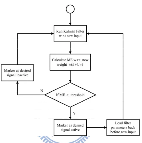
threshold, the current frame is regarded as voice inactivity and thus the parameters update is preserved with respect to current frame. The flow chart of the voice activity detection procedure is as Fig 2.

Fig. 2 Flow Chart of Voice Activity Detection Procedure

It has to be note  v

ise d that the Measurement Error is not discriminative enough if is ill-chosen. Since the the critical error term is the Measurement Error on no reduction,  should be chosen large enough to spare efforts on noise reduction. v However, the best  should consider both noise reduction and dereverberation, so v the appropriate  ould not be chosen extremely large. To overcome such dilemma, v two Kalman filters should be executed, one with large v

sh

 that executing noise

reduction and detecting signal activity while another one with medium  that v computes optimal weight w(k,w) to achieve best tradeoff between noise reduction

and dereverberation.

3.6 Threshold Decision and SINR Estimation

e voice activity is not deter

In Section 3.5, the threshold that discriminates th

mined. In Section 3.6.1, the procedure that determines the threshold will be presented. In Section 3.6.2, the result of the detection procedure can be further reused to estimated current SINR and help choosing the best  , which is undetermined in v Section 3.4.

3.6.1 Gaussian Mixture Model and EM Algorithm

orated to guide the data class

p

The Gaussian Mixture Model (GMM) is incorp

ification [9]. The distribution of Measurement Error when signal is inactive is modeled as a Gaussian distribution and the distribution of Measurement Error when signal is active is modeled as another Gaussian distribution as Fig. 3. This model is described by the following equations. Let xk denote the first element of the Measurement Error at time k. z is the speech/nonspeech label, z{0,1}, where 0 denotes nonspeech and 1 for s eech. According to Bayes’ Rule, it can be written that

), ( ) , ( ) , ( ) (x p x z p x z p z p _{k k k} z z





     (3.21)

where p(z) is the prior probability of speech/nonspeech, and is coeff

actually equal to the weight icient wz (w0 w1 1). p(xk z,) represents the likelihood of xk given speech/nonsp ch mee odel.

} 2 / ) ( exp{ 2 1 ) , ( k z 2 z z k z x x p        (3.22)

where  and z  denotes the mean and variance respectively. z  {z,z,wz z0,1} is the parameter set of the GMM.

Fig. 3 Schematic illustration of error distribution: (a) Distribution of noisy speech; (b) Distributions of speech and nonspeech (This Figure is modified from [9]) Let be a sequence of the first element of the Measurement Error. The probability density function (PDF) is given by

} , , {x0 x1 x2xM  x



  M k k x p p 0 ) ( ) (x  . (3.23)

The parameter set  is estimated by maximizing the above PDF function. From the GMM, both of the PDFs of speech and nonspeech can be obtained, namely p( z 1,)p(z1) and p( z 0,)p(z 0). These two PDFs are shown in Fig. 3(b). From the two PDFs, the optimal threshold  can be obtained to minimize the classification error. The threshold  satisfies

) 0 ( ) , 0 ( ) 1 ( ) , 1 ( z p z  p z  p z  p     (3.24) Eq. (3.24) is a quadratic equation with one unknown . The threshold is one of its roots location between the two means, namely 1  0. The samples with error less

3(b) denotes the classification error.

The crucial issue of the above model is to estimate the parameter set . The estimation consists of an initialization and a sequential updating process. The initial GMM is first established by the EM algorithm, and then incrementally updated with coming data. The parameter set at time k is denoted as _k {_k,z,_k,z,w_k,z z0,1}.

0

 is the initial parameter set estimated from the first M samples by EM algorithm.

According to [9], the following are the typical EM re-estimation formulas,



 z j z j z j z x p w z x p w x z p ) , ( ) , ( ) , (    (3.25)



   1 0 ) , ( 1 ' M j j z p zx M w  (3.26) ' ) , ( ' 1 0 z M j j j z Mw x z p x



     (3.27) ' ) , ( ) ' ( ' 1 0 2 z M j j z j z Mw x z p x



       (3.28)

, where '~{w_z',_z',_z'} is the new parameter set re-estimated from . In the next iteration,  is replaced by '. This iteration continues until EM algorithm converges. The final ' is the initial parameter set  required to GMM initialization and the 0

threshold  can be obtained by solving (3.24).

According to [9], it assumes the GMM varies with time slowly, k k1 at time

. Accordingly, the relationship

k





        k K k j k j k K k j k j p zx x z p 1 1 1 ) , ( ) , (   . The summation is

approximated by the zero-order moment, kz k K k j k j Kw x z p _, 1 ) , ( 



    , where K is a

parameter defined by user which determines the adaption speed. Therefore, the adaption formulas can be written as follows,

) , ( ) 1 ( ₁ , , 1z kz k k k w p zx w _    _  (3.29) z k k k k z k z k z k w x x z p w , 1 1 1 , , , 1 ) , ( ) 1 (            (3.30) z k z k k k k z k z k z k w x x z p w , 1 2 , 1 1 1 , , , 1 ) )( , ( ) 1 (               , (3.31)

where  stands for forgetting factor. Besides, some constraints are required during the adaption process as follows.

} , max{ ,1 ,0 1 ,    k  k k  (3.32) } , max{ ,0 ,1 1 , k k k     (3.33) 1 , 0 , 1 , 1 , 1 } , max{ k k k k w w w w     (3.34)

The reason for constraint (3.32) is based on the inspection that the mean of the Measurement Error when speech is always larger than nonspeech, thus a lower bound for  is implemented by adding a gap k,1  to  and choose the larger one. The k,0

reason for constraint (3.33) is based on the inspection that the variance of the Measurement Error when speech is always not smaller than the the variance of the Measurement Error when nonspeech. The reason for constraint (3.34) is to stem the minimum prior probability of speech from becoming 0 and inducing no adaption afterwards, where  is also a parameter to be chosen.

initialization and adaption. The process of EM algorithm is written in Fig. 4 and the total procedure of VAD decision is written as Fig. 5.

Initialize GMM by using unsupervised clustering while GMM likelihood is increasing

if wk,1

wk,1 

wk,0 1

break end

Calculate p(zxj,) for all and z xj with (3.25) Calculate new weights with (3.26)

Calculate new means with (3.27) Constraint means with (3.32)

Calculate new variances with (3.28) Constraint variances with (3.33) end

Fig. 4 EM algorithm with constraints (revised from [9])

for the first M frames

Calculate the Measurement Error

Establish a GMM by EM with constraints

Determine the threshold from GMM using (3.24) Classify M frames as speech/nonspeech

Discriminate speech/nonspeech by hangover scheme end

for new frame at time k1

Calculate the Measurement Error Calculate p(zx_j,) with (3.25)

Update the weight coefficients with (3.29) Constraint the weight coefficient with (3.34) Update the means with (3.30)

Constraint the means with (3.32) Update the variances with (3.31) Constraint the variances with (3.33)

Determine the threshold from GMM using (3.24) Determine xk1 as speech/nonspeech

end

Fig. 5 The process of VAD decision (revised from [9]) Fig. 5 The process of VAD decision (revised from [9])

3.6.2 SINR Estimation

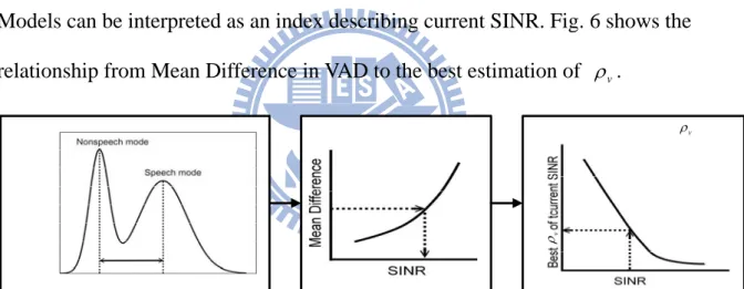
In Section 3.4, the best  that determines the tradeoff between noise reduction v and dereverberation is undetermined. It is mentioned that it should be related to the current SINR since  leverages the effort to reduce noise and enhance signal while v SINR stands for the ratio of signal power and noise power. From the result of Section 3.6.1, the two Gaussian Models stand for the Measurement Error of signal part and noise part, which is also can be related to SINR. The mean of the Gaussian Model for signal and noise can be regarded as two indices describing the signal power and noise power after adaptive filtering. Therefore, the mean difference of the two Gaussian Models can be interpreted as an index describing current SINR. Fig. 6 shows the relationship from Mean Difference in VAD to the best estimation of  . v

v



v



Fig. 6 The relationship from Mean Difference in VAD to the best estimation of  v

In Fig. 6, there are three blocks used to determine the best estimation of  . The v first block is calculating the mean difference from current GMM, which is trivial after building the Gaussian Mixture Models.

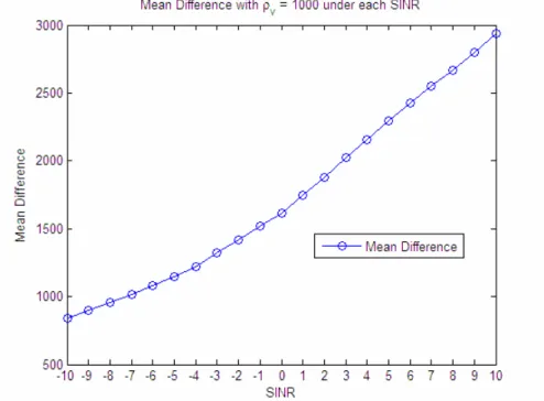
The second block is estimating the current SINR by current Mean Difference. Although the conceptual relationship can be imagined, there is still no concrete equation to describe the relationship between them. To solve that problem, the relationship can be pre-trained. The curve, or the relationship, can be found by mixing

signal clip and noise clip recorded on testing scenario with various amplitudes to acquire clips with different SINRs. With those clips, the computation of computing Measurement Error with Kalman filter and perfect VAD are preceded. After the computation and building GMM modles, the Mean Difference can be found corresponding to the testing clips. Finally, rearranging the correspondence from SINR to Mean Difference, the relationship can be trained. An example showing the result of a series of training is in Fig. 7. With the relationship from SINR to Mean Difference, it can be used to inversely look up when requiring current SINR given Mean Difference.

Fig. 7 An example of trained relationship from SINR to Mean Difference

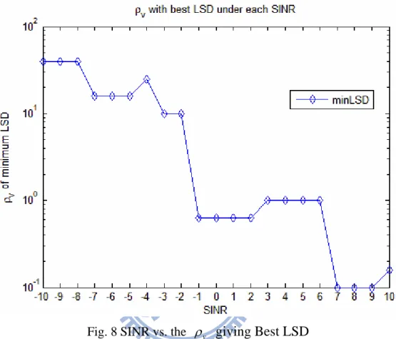
The third block is estimating the best  corresponding to current SINR. It can v also be trained to build the relationship. The pre-training procedure is varying  v from 0.01 to 100 with multiplication of 100.2 for each sample clip of different SINR and finding the best output. The “best output” can be measured by some combination of objective indices like output SINR or log spectrum distortion (LSD). An example of

giving the best output by minimizing the LSD through various  and various SINR v is presented in Fig. 8. Note that small LSD stands for less distortion and high signal quality.

Fig. 8 SINR vs. the  giving Best LSD _v

With the Gaussian Mixture Models and the two pre-trained blocks, the best  v under that trained scenario can be founded.

3.7 Overall System Architecture

Combining the beamforming technique proposed in Section 3.3, the voice activity detection in Section 3.5 and the parameter determinism in Section 3.6, the overall system architecture is presented in this section.

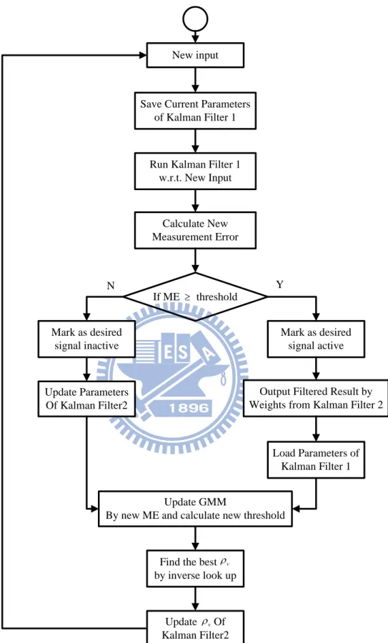
The flow chart Fig. 9 is plotted to elaborate the overall system architecture. The main processing can be separated to two Kalman filters, written as Kalman filter 1 and Kalman filter 2 in Fig. 9 The Kalman filter 1 is operated as the voice activity detector,

thus its  should be chosen large enough to place appropriate efforts on noise v reduction. By a large  , the Measurement Error will be discriminative enough to v separate the signal part and noise part. The Kalman filter 2 serves as the beamformer, so its  should be chosen appropriately to balance the tradeoff between noise v reduction and dereverberation.

To start with, new speech samples in time domain are collected in frames with fixed overlap to the previous frame and transformed to frequency domain after zero padding and Hanning windowing. Before feeding the new frame to Kalman filter 1, the old parameters of Kalman filter 1 is preserved in case later the Measurement Error shows the Kalman filter 1 should not adapt to the new frame since it contains desired signal. After saving current parameters of Kalman filter 1, the Kalman filter 1 tries to adapt itself to the new frames and calculate the Measurement Error with respect to the new frame. The Measurement Error is compared with the threshold and used to

determine the new frame is desired signal active or inactive.

If the new frame is determined as desired signal active, it should be weighted and summed by the weightings given by Kalman filter 2. As mentioned before, the Kalman filter 2 serves as beamformer and filters out undesired noise and maintains desired signal undistorted. After giving filtered result, the parameters of Kalman filter 1 should be loaded by the parameters before adapting to new frame, since the new frame

contains desired signal and should not be adapted by Kalman filter 1.

If the new frame is determined as desired signal inactive, it should be fed to Kalman filter 2 to adapt to the noise contained in the new frame. During the adaption phase, the parameters will be meanwhile updated.

New input

Run Kalman Filter 1 w.r.t. New Input If ME threshold Mark as desired signal active  Y N

Save Current Parameters of Kalman Filter 1

Calculate New Measurement Error

Output Filtered Result by Weights from Kalman Filter 2 Mark as desired signal inactive Update Parameters Of Kalman Filter2 Load Parameters of Kalman Filter 1 Update GMM

By new ME and calculate new threshold

Find the best by inverse look up v  Update Of Kalman Filter2 v 

After determining the voice activity, the new Measurement Error is used to update the GMM and calculate for new threshold. The Mean Difference of the two Gaussian Models can be used to look up for current SINR and the best  for Kalman filter 2. v

To sum up with, the overall algorithm contains two Kalman filters to handle the two issues of voice activity detection and beamforming respectively. The two Kalman filters differ in its crucial parameter  and thus render different functions and v scenarios. The GMM is incorporated to help detecting voice activity and separate the signal and noise as two groups, which gives more information to retrieve the best  v corresponding to current SINR.

Chapter 4. E

XPERIMENT

R

ESULTS

4.1 Introduction of the Experiment Condition

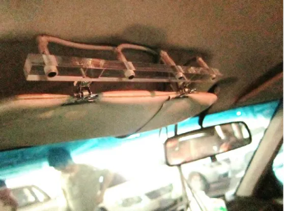
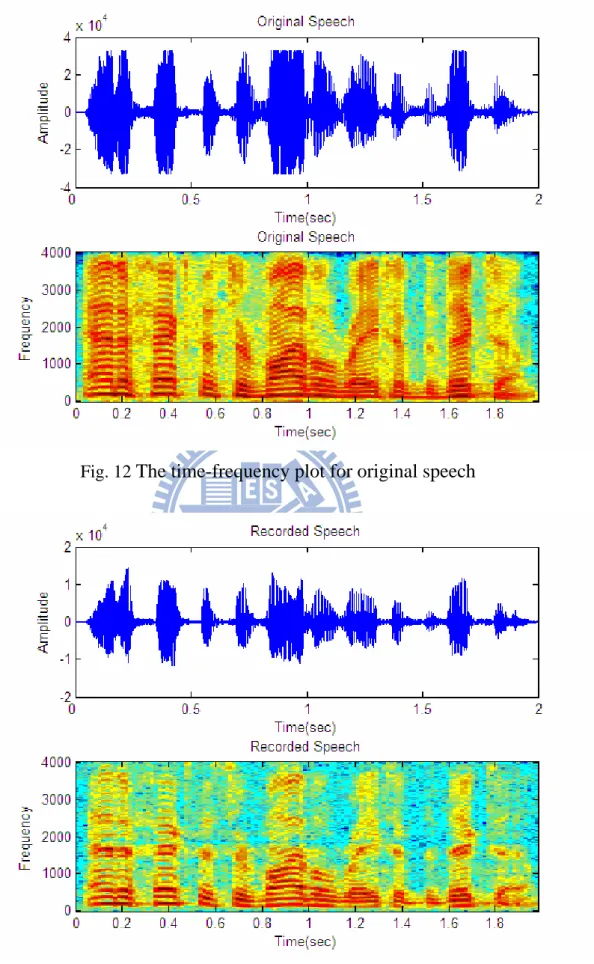
In the experimental results presented afterward, the original sound samples are recorded in a Ford Fiesta car by a microphone array placed at the sun shield of driver’s seat. The desired male speech is played by the Head and Torso Simulator (HATS) by Brüel & Kjær on the driver’s seat. The speech data is extracted from a listening comprehension test by an English learning center, thus giving high SNR. The interfering female speech is played by the same HATS on the copilot’s seat. It is also extracted from an English listening comprehension test. The noise is recorded when the car is driving on road with speed at around 50 km/hr. More specifications about the experiment are presented in Table 1. The photos illustrating the recording environment are as Fig. 10 and Fig. 11. Fig. 12 and Fig. 13 are the time-frequency plots from the known clips played and the signal clips recorded, both of which are used as reference signal in this experiment.

Microphone Number 4 Microphone Displacement 7 cm

Sampling rate 8000 Hz FFT size 512 samples

Shift number 160 samples Zero padding 32 samples

Table 1 Parameters in experiment

The sound data is recorded by a digital microphone array, which uses digital microphones to receive signal and collects 16-bits array data in an Altera FPGA development board. The received data is visible for an embedded network hardware NetBurner through shared memory. Finally, the array data is transferred to PC or Laptop through Local Area Network (LAN).

Fig. 10 The photo for the microphone array at the sun shield of the driver’s seat.

Fig. 12 The time-frequency plot for original speech

4.2 Experiments on Performance of Noise Reduction and Its

Tradeoff with Dereverberation

In this section, the tradeoff phenomenon between noise reduction and dereverberation is exhibited. The experiment environment is as mentioned in Section 4.1. Three speech enhancement algorithms, MVDR, MVDR with Kalman filter solution, DSB (Delay and Sum Beamformer) are implemented to compare with proposed algorithm. In this section, perfect voice activity detection is assumed for MVDR, MVDR with Kalman filter and proposed algorithm to avoid sample matrix inverse (SMI) problem [10]. For the MVDR filter, the forgetting factor of sample covariance matrix is 0.99. In proposed beamformer, the parameter  ranges from v 0.001 to 1000 with ration of increase 10.

Two objective performance indices are used to measure the waveform property. The first is the average SINR (avgSINR) defined as







     n n T t n T t n Ts t s t x T t x T t x T ) ( 1 ) ( 1 ) ( 1 avgSINR 2 2 2 (4.1)

where and denote periods in time when only the desired speech is active and only the interference-plus-noise signals are active respectively. The second quality measure is log spectral distortion (LSD) defined as

s T T_n





    K k W w r k w Y k w s W K 1 1 2 10 10 ( , ) 10log ( , )) log 10 ( 1 1 LSD (4.2)

where is the Short-time Fourier transform (STFT) of the original sound played by HATS and is the STFT of the beamformer output. LSD means the

) , (k w sr ) , (k w Y

speech distortion in frequency domain. Note that a lower LSD level corresponds to better performance.

In Fig. 14(a), Fig. 15(a) and Fig. 16(a), the effect of  regarding SINR is as v expected. Higher  gives higher noise reduction level and thus giving better v performance. In contrast, small  gives low noise reduction level and thus giving v bad result in LSD since noise and distortion both worsen the LSD. Since the perfect voice activity detection is assumed, other methods like MVDR and MVDR with Kalman filter both performs well. With perfect voice activity detection, the MVDR works on perfect situation that signal correlation matrix and noise correlation matrix are perfectly identified. In that case, its solution is close to optimal solution for maximizing output SINR. However, in Fig. 14(b), Fig. 15(b), Fig. 16(b) the LSD shows that MVDR and MVDR with Kalman filter are suffered from distortion while proposed algorithm works better if  is chosen appropriately. v

For subjective evaluations, Fig. 17, Fig. 18 and Fig. 19 show the waveforms and spectrograms at different SINR -2 dB, 4 dB and 7 dB. It can be observed that both in MVDR and DSB, the voice pattern in frequency domain is still preserved while proposed method and MVDR with Kalman filter somehow blurred the voice pattern in frequency domain. Regarding the noise reduction, it can be observed that most of the noises are eliminated in proposed method, MVDR and MVDR with Kalman filter.

(a) avgSINR result (b) LSD result Fig. 14 Experiment results in car environment with input SNR 7 dB

(a) avgSINR result (b) LSD result Fig. 15 Experiment results in car environment with input SNR 2 dB

(a) avgSINR result (b) LSD result Fig. 16 Experiment results in car environment with input SNR -4 dB

(a) Original Speech (b) Contaminated Speech

(c) Proposed Algorithm (d) MVDR+Kalman

(e) MVDR (f) DSB

(a) Original Speech (b) Contaminated Speech

(c) Proposed Algorithm (d) MVDR+Kalman

(e) MVDR (f) DSB

(a) Original Speech (b) Contaminated Speech

(c) Proposed Algorithm (d) MVDR+Kalman

(e) MVDR (f) DSB