行政院國家科學委員會專題研究計畫 成果報告
後次微米時代新興電子設計自動化技術之研究--子計畫
二:整合性低耗電管理之技術開發(3/3)
研究成果報告(完整版)
計 畫 類 別 : 整合型 計 畫 編 號 : NSC 99-2220-E-009-009- 執 行 期 間 : 99 年 08 月 01 日至 100 年 07 月 31 日 執 行 單 位 : 國立交通大學電子工程學系及電子研究所 計 畫 主 持 人 : 江蕙如 計畫參與人員: 碩士班研究生-兼任助理人員:詹雅仲 碩士班研究生-兼任助理人員:何松庭 碩士班研究生-兼任助理人員:蔡昌澄 碩士班研究生-兼任助理人員:譚傳耀 大專生-兼任助理人員:張之龍 博士班研究生-兼任助理人員:李婉毓 博士班研究生-兼任助理人員:楊喻名 博士班研究生-兼任助理人員:余彥廷 公 開 資 訊 : 本計畫涉及專利或其他智慧財產權,2 年後可公開查詢中 華 民 國 100 年 10 月 31 日
中文摘要: 近年來,耗電量已成為必需正視的課題。產品的趨勢方面,時 脈頻率不斷攀升、功能需求不停添加以及體積更加輕巧;製程 的演進趨勢方面,供應電壓持續下降,直接而有效的降低動態 耗電,但是從這部分所能得到的好處卻趨於緩和,甚至漸漸出 現了負面效應(漏電流的效應成指數型式成長);兩相加乘的 結果,使得耗電密度(power density,power-per-area)與日俱 增。根據 2006 年更新的 ITRS 所預估:耗電的問題從 2007 年 開始變成不可不解的困擾,到了 2017 年會陷入更深的困境。低 耗電管理的技術的發展,時至今日已有一段時間,就系統層級 (system-level)而言,動態電壓與頻率調節(dynamic voltage and frequency scaling,DVFS)與動態電源管理(dynamic power management,DPM)為兩種最為廣泛應用的技術。 動態電壓與頻率調節技術為多重供應電壓的延伸,不僅是空間 軸上(block domain)甚至是時間軸上(time domain)都可以 應用,每個區域因工作模式的不同可以有不同的時序要求。所 以在 critical 的時候/區域使用高電壓、高頻時脈;在 non-critical 的時候/區域使用低電壓、低頻時脈;而動態電源管理 技術會根據時間軸上目前的工作多寡來調整晶片的工作能力。 當工作多時,晶片會處在高計算能力╱高功耗的狀態,當工作 量少時,晶片會處在低計算能力╱低功耗的狀態,而當無工作 時,晶片將會進入閒置狀態,以此種動態調整來降低處理完一 定工作量之功耗。 而近來,因對系統的效能要求,多核心處理器(multicore proccessor)也日漸受到重視,藉由將數個相同的核心(core) 整合,能在不大幅增加功耗的情況下,達到一定水準的效能。 在多核心處理器的架構下,可以將動態電壓與頻率調節與動態 電源管理來做結合:每個核心擁有自己的電壓島(voltage island)及頻率島(frequency island),因此在同一時間點下, 每個核心能處在不同的電壓╱頻率;由每個核心的電壓╱頻 率,可以得到目前處理器的功率狀態(power state)。動態電 源管理將視當下的工作量來決定處理器的功率狀態,而動態電 壓與頻率調節會依目前處理器的功率狀態,來配置每個核心的 工作電壓及頻率。 動態電源管理的研究雖已行之有年,但是大部份的解決方法都 只對特定的工作行為有效用,但實際上,工作的行為特徵並無 法在事前預知,因此,動態電源管理技術的彈性及其對不 3 同工作行為特徵的適應能力為管理技術是否有效的一大重點。 為了使動態電源管理技術達到良好的彈性及適應能力,在本計 畫中,我們採用增強式學習法(reinforcement learning)來做為
(environment)的互動及衡量,由代理人做出最有益整體的選 擇,換句話說,即使面對相同的問題,代理人每次做的選擇不 一定會相同,但一定是當時環境下最有益的選擇;其優良的彈 性及適應能力,將大大增進動態電源管理的效能。同時,我們 也提出一套將多核心處理器的功率狀態減化並優化功耗的技 術,讓動態電源管理時間及空間的複雜度降低。 在本計畫中,我們提出了一套動態電源管理的工具,其貢獻如 下: 1. 在多核心處理器上,整合了動態電源管理與動態電壓與頻率 調節。 2. 運用增強式學習法的彈性及適應能力來做動態電源管理。 3. 將多核心處理器的功率狀態減化並優化功耗,讓動態電源管 理的複雜度降低。
英文摘要: Power consumption has become a critical issue in modern VLSI design. Dynamic voltage and frequency scaling (DVFS) and dynamic power management (DPM) are two attractive solutions at system level. Unlike prior works that adopt offline techniques or are restricted to a single core processor, in this work, we combine DVFS with DPM together and propose an online DPM
methodology to multicore processors. Our method is based on reinforcement learning and Markov decision process. With state reduction, we avoid state explosion and simplify the learning mechanism. Experimental results show that the number of states is greatly reduced, but the effectiveness of our DPM is still
maintained. We apply our DPM on a quad core processor; our DPM method can achieve 20% power reduction on average without delay penalty.
行政院國家科學委員會補助專題研究計畫
■ 成 果 報 告
□期中進度報告
後次微米時代新興電子設計自動化技術之研究-
子計畫二:整合性低耗電管理之技術開發(3/3)
計畫類別:□ 個別型計畫 ■ 整合型計畫
計畫編號:NSC 99-2220-E-009-009
執行期間: 97 年 8 月 1 日至 100 年 7 月 31 日
計畫主持人:江蕙如助理教授 國立交通大學電子工程學系
共同主持人:
計畫參與人員:
成果報告類型(依經費核定清單規定繳交):□精簡報告 ■完整報告
本成果報告包括以下應繳交之附件:
□赴國外出差或研習心得報告一份
□赴大陸地區出差或研習心得報告一份
□出席國際學術會議心得報告及發表之論文各一份
□國際合作研究計畫國外研究報告書一份
處理方式:除產學合作研究計畫、提升產業技術及人才培育研究計畫、列管
計畫及下列情形者外,得立即公開查詢
□涉及專利或其他智慧財產權,□一年■二年後可公開查詢
執行單位:國立交通大學電子工程學系
2
一、中文摘要
近年來,耗電量已成為必需正視的課題。產品的趨勢方面,時脈頻率不斷攀升、功能需求 不停添加以及體積更加輕巧;製程的演進趨勢方面,供應電壓持續下降,直接而有效的降低動 態耗電,但是從這部分所能得到的好處卻趨於緩和,甚至漸漸出現了負面效應(漏電流的效應 成指數型式成長);兩相加乘的結果,使得耗電密度(power density,power-per-area)與日俱 增。根據 2006 年更新的 ITRS 所預估:耗電的問題從 2007 年開始變成不可不解的困擾,到了 2017 年會陷入更深的困境。低耗電管理的技術的發展,時至今日已有一段時間,就系統層級 (system-level)而言,動態電壓與頻率調節(dynamic voltage and frequency scaling,DVFS) 與動態電源管理(dynamic power management,DPM)為兩種最為廣泛應用的技術。動態電壓與頻率調節技術為多重供應電壓的延伸,不僅是空間軸上(block domain)甚至 是時間軸上(time domain)都可以應用,每個區域因工作模式的不同可以有不同的時序要求。 所以在 critical 的時候/區域使用高電壓、高頻時脈;在 non-critical 的時候/區域使用低電壓、 低頻時脈;而動態電源管理技術會根據時間軸上目前的工作多寡來調整晶片的工作能力。當工 作多時,晶片會處在高計算能力╱高功耗的狀態,當工作量少時,晶片會處在低計算能力╱低 功耗的狀態,而當無工作時,晶片將會進入閒置狀態,以此種動態調整來降低處理完一定工作 量之功耗。 而近來,因對系統的效能要求,多核心處理器(multicore proccessor)也日漸受到重視, 藉由將數個相同的核心(core)整合,能在不大幅增加功耗的情況下,達到一定水準的效能。 在多核心處理器的架構下,可以將動態電壓與頻率調節與動態電源管理來做結合:每個核心擁
有自己的電壓島(voltage island)及頻率島(frequency island),因此在同一時間點下,每個核
心能處在不同的電壓╱頻率;由每個核心的電壓╱頻率,可以得到目前處理器的功率狀態
(power state)。動態電源管理將視當下的工作量來決定處理器的功率狀態,而動態電壓與頻率
調節會依目前處理器的功率狀態,來配置每個核心的工作電壓及頻率。
動態電源管理的研究雖已行之有年,但是大部份的解決方法都只對特定的工作行為有效 用,但實際上,工作的行為特徵並無法在事前預知,因此,動態電源管理技術的彈性及其對不
同工作行為特徵的適應能力為管理技術是否有效的一大重點。為了使動態電源管理技術達到良 好的彈性及適應能力,在本計畫中,我們採用增強式學習法(reinforcement learning)來做為 控制核心。增強式學習法藉由代理人(agent)與環境(environment)的互動及衡量,由代理 人做出最有益整體的選擇,換句話說,即使面對相同的問題,代理人每次做的選擇不一定會相 同,但一定是當時環境下最有益的選擇;其優良的彈性及適應能力,將大大增進動態電源管理 的效能。同時,我們也提出一套將多核心處理器的功率狀態減化並優化功耗的技術,讓動態電 源管理時間及空間的複雜度降低。 在本計畫中,我們提出了一套動態電源管理的工具,其貢獻如下: 1. 在多核心處理器上,整合了動態電源管理與動態電壓與頻率調節。 2. 運用增強式學習法的彈性及適應能力來做動態電源管理。 3. 將多核心處理器的功率狀態減化並優化功耗,讓動態電源管理的複雜度降低。 關鍵詞:動態電源管理;動態電壓與頻率調節;多核心處理器;增強式學習
二、計畫的緣由與目的
I. INTRODUCTIONAs technology advances into nanometer era, power consumption is a crutial issue in VLSI design. Several well-developed techniques are proposed to alleviate this issue. Among them, dynamic voltage and frequency scaling (DVFS) and dynamic power management (DPM) are two popular solutions at system level [1].
4
DVFS is a process to dynamically modify the supply voltage and the operating frequency. We boost the timing critical part of design with a higher voltage-frequency (V-F) setting to meet the performance requirement while slow down the non-critical part with a lower V-F setting to reduce the power consumption (referred to dynamic power in this work). Since power consumption is directly proportional to the operating frequency and quadratically proportional to the supply voltage, DVFS achieves a cubic reduction in power consumption.
On the other hand, DPM is a procedure to dynamically adjust the computational ability of a device according to the workload applied on it. DPM slows down or turns off the device when no work is (predicted to be) coming. In other words, the computational ability of a device is reduced as it is idle. As a result, if DPM manages well, the power consumption of the idle period can be saved while the performance is maintained.
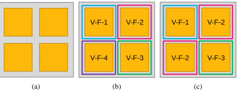
In order to provide high performance with acceptable power consumption, a multicore processor (a.k.a. chip multiprocessor, CMP) is developed, which integrates numbers of monotonic cores into one chip. Figure 1(a) depicts a multicore processor with four identical cores. With DVFS, each core on this multiprocessor can be assigned with a specific V-F setting according to its workload. Four different V-F settings {V-F-1, V-F-2, V-F-3, V-F-4} are applied on each core in Figure 1(b), while three V-F settings are applied in Figure 1(c). (V-F-2 is applied on two cores, while V-F-1 and V-F-3 is applied on one core, respectively.) With different V-F settings, the processor shows different statuses in computational ability and power consumption. Furthermore, if we consider each circumstance as a
V-F-4 V-F-1 V-F-3 V-F-2 V-F-2 V-F-1 V-F-3 V-F-2 (a) (b) (c)
Figure 1. (a) Multicore processor. (b) 4 cores with 4 different DVFS settings {V-F-1, V-F-2, V-F-3, V-F-4}. (c) 4 cores with 3 different DVFS settings.
state of processor, we can combine DVFS and DPM together. The states are constructed by DVFS, and the transitions between states are guided by DPM.
In literature, most of prior works proposed DPM and DVFS for a single core or functional unit [2-9]. Only few works [10-11] can handle multicore processors, but they need offline processing. Chung et al. proposed a timeout policy that turns off the device when an idle period is long enough in [2], while Hwang and Wu adopted exponential average to predict the length of idle periods in [3]. A single policy, e.g., the timeout policy [2] or the exponential predictive policy [3], only performs well under a certain workload. In [4], Qiu and Pedram regarded the environment as a stochastic model and found the optimal policy iteratively. However, the stochastic policy like [4] loses its optimality when workload becomes non-stationary. Dhiman and Rosing combined several policies and designed an expert to choose the best policy for each period in [5], [6] and [7]. Nevertheless, the performance of the expert-based policy [5-7] heavily relies on the effectiveness of the pre-defined experts. Recently, some works modeled this problem as Markov decision process and used machine learning to perform DPM because it can provide the adaption and the flexibility to different kinds of workloads [8-10]. Tan et al. constructed a power manager for a hard disk drive by modified Q-learning in [8], while Wang et al. built it by reinforcement learning in [10]. Jung and Pedram used supervised learning as DPM for multicore processors [9]. However, supervised learning needs to extract data and execute training offline, e.g., [9]. Moreover, [8], [9] and [10] adopted the state model including a service requestor, a service queue and a service provider as well as the probability distribution. In consequence, the number of states is considerable and the overhead in computation is high. The possible state explosion problem results in runtime penalty and causes previous machine learning based DPM hard to be embedded in high performance designs, such as multicore processors. In addition, Kolpe et al. applied clustered DVFS on multicore processors but found the clusters offline in [11].
6
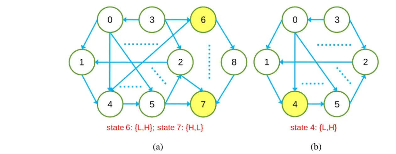
Unlike previous works, we propose an online DPM method to dynamically alter V-F settings of a multicore processor by adopting reinforcement learning in this work. Our method is based on Markov decision process while the number of states is greatly reduced. Our DPM does not include service requestor, service queue and service provider in the state model and thus simplifies the learning mechanism. In addition, our work guarantees the minimum transitions between states. This feature allows us to reduce the number of states as well as power consumption. Figure 2 illustrates an example of state reduction on a duo core processer, in which each has 3 V-F settings: {high (H), low (L), sleep (0)}. The states in Figure 2(a) are constructed by the permutation of V-F settings. Thus, there are 9 (=3*3) states: {{0, 0}, {0, L}, {0, H}, {L, 0}, {H, 0}, {L, L}, {L, H}, {H, L}, {H, H}}. As shown in Figure 2(b), with the proposed state reduction, each state is encoded by the number of cores under each V-F setting. Therefore, as shown in Figure 2(b), we have only 6 states: {{0, 0}, {0, L,}, {0, H}, {L, L}, {L, H}, {H, H}}. With the proposed state reduction, the number of states can be greatly reduced from 9 (see Figure 2(a)) to 6 (see Figure 2(b)), and the transitions between states are also minimized. Please note that, as the number of cores and available V-F settings increases, the state model like Figure 2(a) will face the state explosion issue. Moreover, our state reduction method can largely simplify our learning mechanism. Hence, our method is more suitable for multicore
6 7 8 0 1 4 3 2 5 …… ……… ……… state 6: {L,H}; state 7: {H,L} 0 1 4 3 2 5 …… ……… state 4: {L,H} (a) (b)
Figure 2. State reduction. Consider a duo core processer; each core has 3 possible V-F settings: {high (H), low (L), sleep (0)}. (a) Without state reduction. Totally 9 states. (b) With state reduction. Totally 6 states. It can be seen that two or more states can be merged into one, e.g., {L, H} and {H, L} has the same computational ability and power consumption.
processors.
II. PRELIMANARIES AND PROBLEM FORMULATION
We first briefly introduce reinforcement learning and Markov decision process and then give the problem formulation.
A. Reinforcement Learning
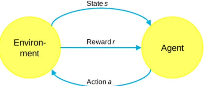
Reinforcement learning (RL) is a machine learning technique that depends on interactions between an agent and the environment (see Figure 3). The agent observes the state of the environment, evaluates the rewards (costs) it can get if it takes some actions, and chooses the action with the maximum benefit (minimum penalty) to perform. RL mimics the natural learning process of animals and humans [12].
Unlike supervised learning, there are no correct answers in RL. In other words, instead of deciding what is correct and what is incorrect, RL just chooses the side with more benefits. This property makes RL suitable for the problems in which it is very hard to distinguish what is correct and what is wrong, e.g., DPM problems. Moreover, supervised learning needs huge amount of training data and can only be trained offline. The trained supervised learner will not make the best decision once the characteristics of incoming tasks differ from those in training data. As a result, in this work, we use RL to learn our DPM policy.
Environ-ment Agent
State s
Reward r
Action a
8
B. Markov Decision Process
A Markov decision process is a 5-tuple element (S, A, {Psas’}, , R), where S is the set of states, A is
the set of actions, {Psas’} are the state transition probabilities, is the discount factor, and R is the
reward. psas' denotes state sS goes to state s'S by taking action aA. Moreover, the summation of
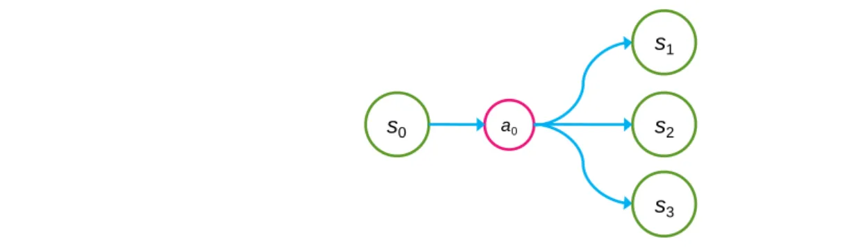
the state transition probability of a given original state through an action will be one. For example, in Figure 4, we have S = {s0, s1, s2, s3} and A = {a0}. The state transition probability
1 0 0a s
s
p gives the
possibility of s0 transfers to s1 through a0, while ps0a0s2, ps0a0s3 represents that to s2 and s3,
respectively, and 2 3 1 0 0 0 0 1 0 0a s sas sas s p p p .
The discount factor, [0, 1), is used to discount the future reward R: SA , where R(s, a) is the reward we can get after taking action a from state s. After n periods (time slots between two consecutive learning), the expected reward can be write down as:
)]. , ( ... ) , ( ) , ( [R st0 at0 R st1 at1 nR stn atn
A policy maps from states to actions (e.g., : SA). If action a = (s) is performed in state s, we may say that a policy is executed. The value function of a policy V(s) is the expected sum of discount rewards of taking policy in an initial state s:
V(s)[R(st0)R(st1)...nR(stn)|s0s,]
s0 a0 s2
s1
s3
Figure 4. States, action, and transitions of Markov decision process. The summation of the state transition probability of a given original state through an action will be one.
If we write down equation (2) as the Bellman equation:
S s s s s s' V p s R s V ' ( ) ' ) ( ) ( ) ( V(s) can be solved efficiently. We define that the optimal value function is the value function of a policy with the maximum reward as
S s sas A a p V s s R s V ' * ' *( ) ( ) max ( ')while the optimal policy as the action that can bring the maximum reward:
S s sas A a p V s s ' * ' *( ) argmax ( ') Hence, we can find the optimal policy by iterative choosing the action bringing the maximum future expected reward and updating value function [13].
C. Problem Formulation
Given the number of cores, available V-F settings of a core, computational ability and power consumption of each V-F setting, and the transition power between V-F settings of a multicore processor, our target is to find a dynamic power management method which minimizes power consumption and performance degradation under running all kinds of applications.
三、研究方法及成果
I. OUR DPM WITH STATE REDUCTION
We detail our DPM methodology as follows. First, our work guarantees the minimum transitions between states and reduces the number of states as well as power consumption. Second, since we do not model the status of queue and the amount of coming tasks, finding the optimal policy in our DPM
10
more suitable for multicore processors. Experimental results in Section IV.B show that the proposed DPM performs better than the DPMs without state reduction.
A. State Reduction
Unlike previous works, we do not model the service requestor, the service queue and the service provider into a state. On the contrary, we treat V-F settings of cores as our state to avoid state explosion. Each state indicates the number of cores under each V-F setting. Different settings which result in the same computational ability and power consumption are viewed as one state. To validate our state reduction, the state transition power is desired to be minimized. In consequence, with state reduction, our work adopts minimum state transition power between states.
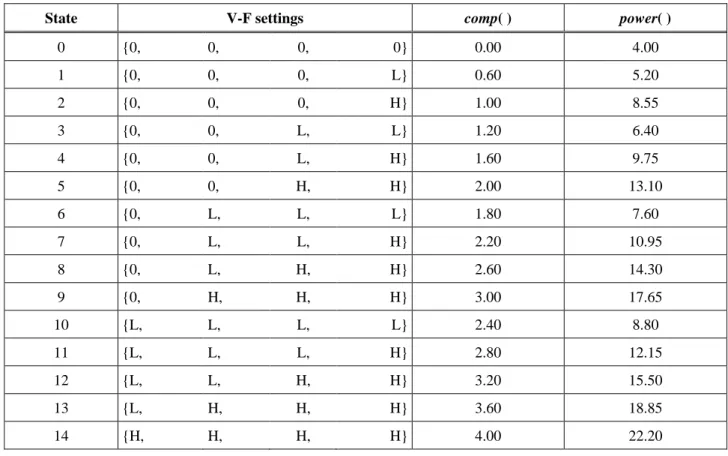
Assume that we conduct our DPM on a quad core processor, and each has three possible V-F settings: high (H), low (L) and sleep (0). Instead of 81 (=34) states, TABLE I lists the 15 states used for this quad core processor, as well as the V-F settings, computational abilities and power consumption. In our work, the state transition power between two states is obtained by the following equations: , ) ' , ( tx LH tx L tx H tx s s p t p t p t p H L LH 0 0 0 0 where ), , min( L H LH d d t ), , min( L LH L d d t t0 0 ). , min( L H LH H d t d t t0 0 0 The notation LH tx
p means the power consumption for a core transferring from L to H, or from H
to L, while
L
tx p
0 stands for the power consumption from 0 to L or L to 0, ptx0H represents that from 0
to H (H to 0). The number of cores transfer from L to H is denoted as tLH and the numbers of cores
in 0, L, H between two states, respectively. Please note that equations (6)-(9) hold under the condition H L LH tx tx tx p p p 0 0 . Assuming that LH tx p = 2.50, L tx p
0 = 3.50 and ptx0H = 5.00, the transition power between state 2 and
state 3 is calculated as follows. First, according to TABLE I, state 2 = {0, 0, 0, H} and state 3={0, 0, L, L}, we know that d0 = 1, dL = 2, and dH = 1. Then, by equations (7)-(9), tLH = 1, t0L = 1, t0H = 0 are
obtained. Finally, we get ptx(s, s') = 6.0 according to equation (6). Moreover, status {0, 0, L, L} and
status {L, 0, 0, L} map to the same state (state 3) in this perspective. Thus, the number of states is further reduced. In other words, instead of permutation, the combination of V-F settings is enough to represent the states of a multicore processor.
B. Proposed Model based on Makov Decision Process
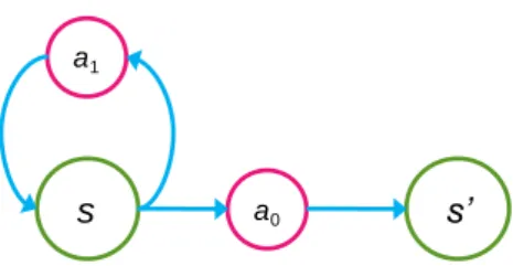
The model used in our work is based on Markov decision process mentioned in Section II.B. As mentioned in Section III.A, we encode a state by the number of cores under each V-F setting. In addition, since we cannot control the status of queue and the amount of coming tasks (both dynamically change according to the application), we embed them in our cost function instead of model them into states. Thus, the number of states can be reduced, and the control over states becomes deterministic, not stochastic like previous works. In consequence, the computing complexity of iteratively finding the optimal policy in our DPM is dramatically reduced. The Markov decision process model used in our work is detailed as follows.
As mentioned above, we model each state by the number of cores under each V-F setting. The
s a0 s’
a1
12
manage the transitions between states: leave and stay. The action leave transports the original state to all the other states, while the action stay remains the next state as the original one. Figure 5 illustrates an example of our model, where the state s transfers to the state s' through the action a0 (leave), while
s remains still when the action a1 (stay) is taken. The state transition probability psas' gives the
possibility of s transfers to s' through a.
Our cost function from the state s to the state s' is defined as follows:
C(s,s')GVa(s')Penalty(s,s'), where G is a factor used to decide how important the historical information of the next state s' is with respect to the penalty can be received right afterwards (same function as discount factor mentioned in Section II.B). The penalty function, Penalty(s, s') is defined as
Penalty(s,s')Power(s,s')MDelay(s'), Power(s,s') ptx(s,s')power(s'), Delay(s')QrQincomp(s').
Power(s, s') contains state transition power ptx(s, s') and power consumption power(s') of the next
period (the time slot between two consecutive learning) when next state is s'. Delay(s') represents how many tasks will remain in queue if the processor is in state s'with computational ability comp(s') when queue already has Qr tasks remained and the number of incoming tasks Qin of next period is the
DPM Learning Adjusting ASTP AG AM
same as the last period. M is the weight between power and delay; it is initially user-specified and adjusted during learning periods (mentioned in Section III.C).
In each evaluation, we choose the policy that minimize the expected cost, i.e.,
S s sas A a p C s s s ' ' ) ' , ( min arg ) ( Moreover, we update the value function
S s s s s C s s p s V ' ( ) ' ) ' , ( ) ( as soon as the evaluation is over.
C. DPM – Finding Policy by Iteratively Learning
Figure 6 illustrates the overflow of the proposed DPM, which is also the agent in RL. Our DPM includes two major parts--learning and adjusting.
Learning: we choose RL as our learning methodology as mentioned in Section II.A and conduct
it on the model proposed in Section III.B. Every learning period, DPM takes the action with the minimum expected cost, and transfers to the state with the minimum cost. DPM basically performs learning every period.
14
Adjusting: three parameters are adjusted online: the state transition probability (ASTP), the G value
used in equation (6) (AG), and the M in equation (7) (AM). ASTP adjusting the transition probabilities every T1 periods by
, _ ' _ ' a count s count psas
where count_a represents how many times action a is taken in s during T1, while count_s' describes
how many times s' is visited when action a taken in s during T1. AG increases G gradually during
learning process. This is because that DPM knows very poor about the interactions with the environment; the penalty function takes the most responsibility for learning. As increasing of learning periods, DPM compiles more and more knowledge of the environment, thus we amplify G and let the experience, i.e., Va(s'), to guide DPM to choose the next state. In addition, AM balances
the importance between power and delay. AM reduces M by m1 if no tasks remains in queue, while
increase it by m2 vice versa. AM guides DPM chooses a state with lower power consumption as task
TABLEI.THE V-FSETTINGS,COMPUTATIONAL ABILITY AND POWER CONSUMPTION OF EACH STATE
State V-F settings comp( ) power( )
0 {0, 0, 0, 0} 0.00 4.00 1 {0, 0, 0, L} 0.60 5.20 2 {0, 0, 0, H} 1.00 8.55 3 {0, 0, L, L} 1.20 6.40 4 {0, 0, L, H} 1.60 9.75 5 {0, 0, H, H} 2.00 13.10 6 {0, L, L, L} 1.80 7.60 7 {0, L, L, H} 2.20 10.95 8 {0, L, H, H} 2.60 14.30 9 {0, H, H, H} 3.00 17.65 10 {L, L, L, L} 2.40 8.80 11 {L, L, L, H} 2.80 12.15 12 {L, L, H, H} 3.20 15.50 13 {L, H, H, H} 3.60 18.85 14 {H, H, H, H} 4.00 22.20
coming rate is light, while prefers a state with more computational ability when task coming rate is heavy. The range of M is from 0.5 to 50. AG and AM performs every T2 and T3 periods, respectively.
II. EXPERIMENTAL RESULTS
A. Settings
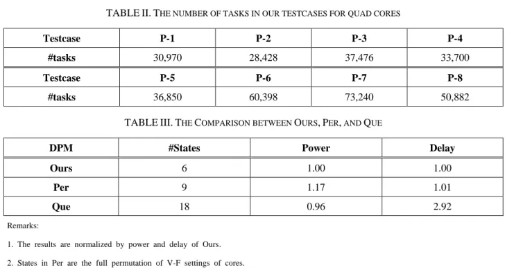
We implement our DPM as a cycle-based simulator using C++. The performance of our DPM is evaluated on 8 testcases generated randomly. TABLE II gives the number of tasks in each testcase on a quad core processor. These cases should be finished within 20,000 cycles. The task incoming rate ranges from 1.42 tasks per cycle to 3.66 tasks per cycle. We did two sets of experiments to show the effectiveness of our method.
B. Effectiveness of State Reduction DPM
In order to show the effectiveness of the state reduction, we conduct experiments on duo core processor. We compare our model with two models, states constructed by full permutation of V-F
TABLEII.THE NUMBER OF TASKS IN OUR TESTCASES FOR QUAD CORES
Testcase P-1 P-2 P-3 P-4
#tasks 30,970 28,428 37,476 33,700
Testcase P-5 P-6 P-7 P-8
#tasks 36,850 60,398 73,240 50,882
TABLEIII.THE COMPARISON BETWEEN OURS,PER, AND QUE
DPM #States Power Delay
Ours 6 1.00 1.00
Per 9 1.17 1.01
Que 18 0.96 2.92
Remarks:
1. The results are normalized by power and delay of Ours. 2. States in Per are the full permutation of V-F settings of cores. 3. States in Que include the status of the queue.
16
model, while 9 in Per and 18 in Que. We categorize the queue into three statuses: low occupancy, medium occupancy, and high occupancy in Que. Besides the state models used, Per and Que have basically the same actions and the same cost functions as ours.
TABLE III shows the comparisons between ours, Per and Que in power and delay under initial M = 9.5. The results are averaged over 8 testcases, as well as normalized by power and delay of Ours, respectively. Since the multicore processor in this experiment has only two cores, we apply half tasks in each cycle for each testcase. It can be seen that our DPM outperforms Per in both power and delay. As expected, Per wastes power on unnecessary transitions. Que has lower power consumption than ours, but degrades performance dramatically. It is because that staying at a wrong state will affect the evaluation of DPM on environment thus making non-optimal decisions. In conclusion, our state reduction reduces complexity of learning while maintains good performance.
C. Performance Evaluation of Proposed DPM Methedology
In the second experiment, we apply our DPM on a quad core processor, e.g., QX9000 series of Intel. We assume that each core has 3 V-F settings including turn-off, i.e., 3.00GHz-1.36V (high performance, H), 1.66GHz-1.13V (low performance, L), and 0GHZ-0.85V (sleep, 0). TABLE I lists the processor states constructed by these four cores and three V-F settings, as well as the computational ability and power consumption of each state. The computational ability comp() is
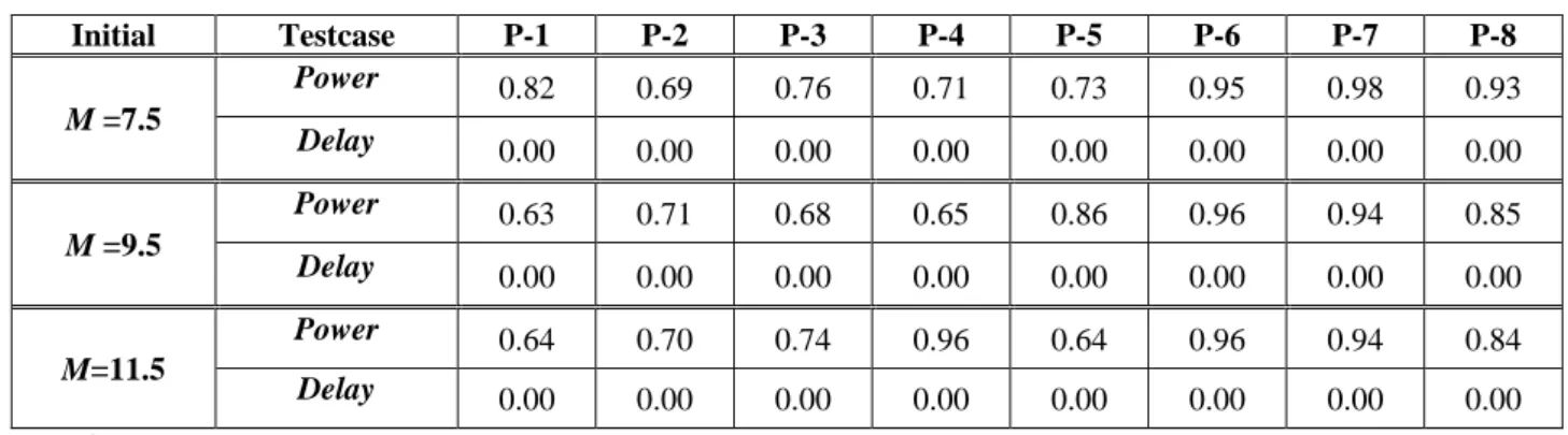
TABLEIV.POWER AND DELAY UNDER DIFFERENT INITIAL M OF OUR DPM
Initial Testcase P-1 P-2 P-3 P-4 P-5 P-6 P-7 P-8 M =7.5 Power 0.82 0.69 0.76 0.71 0.73 0.95 0.98 0.93 Delay 0.00 0.00 0.00 0.00 0.00 0.00 0.00 0.00 M =9.5 Power 0.63 0.71 0.68 0.65 0.86 0.96 0.94 0.85 Delay 0.00 0.00 0.00 0.00 0.00 0.00 0.00 0.00 M=11.5 Power 0.64 0.70 0.74 0.96 0.64 0.96 0.94 0.84 Delay 0.00 0.00 0.00 0.00 0.00 0.00 0.00 0.00 Remarks:
1. Power ratio and delay overhead are normalized to the results obtained by running at state 14. 2. 1 period = 10 cycles. T1 = 184, T2 = 220, T3 = 50 periods.
3. Initially G = 0.1 and increased by 0.1 every 220 periods until G = 1.0. 4. m1 = 0.5; m2 = 0.5. M ranges from 0.5 to 50.
normalized by the size of a task, while the power power() is normalized by the power of a core as it sleeps. There are two actions, leave and stay, as mentioned in Section III.B. Since our DPM guarantees the minimum transition power between states, the transition power ptx(s, s') can be
obtained by equations (6)-(9) in Section III.A. In our work, we set LH tx p = 2.50, L tx p 0 = 3.50 and ptx0H= 5.00. In addition, we set one learning period as 10 cycles and perform ASTP, AG, AM every 184 (T1),
220 (T2), 50 (T3) periods, respectively. We initialize G = 0.1 and increase G by 0.1 every 220 periods
until G = 1.0. AM reduces M by 0.5 (m1) if no tasks remains in queue, while increase it by 0.5 (m2)
every 50 periods. The range of M is from 0.5 to 50.
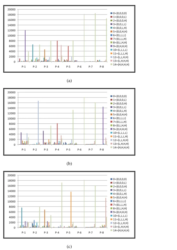
The results of power ratio (Power) and delay overhead (Delay) under different initial M values are detailed in TABLE IV. The results in TABLE IV are normalized to the power and delay obtained if the multicore processor runs in the state with the highest computational ability, i.e., the state 14 with V-F setting = {H, H, H, H}. Figure 7 illustrates the distribution of states under different initial M values of each testcase. The x-axis shows each testcase, the y-axis shows the number that each state is applied on multicore processor, and the bars with different colors represent the states. On average, our DPM saves 18% power consumption under initial M = 7.5, while 22% under M = 9.5, and 20% under
M = 11.5. In general, a higher initial value of M causes DPM to prefer the state with more
computational ability resulting in higher power consumption. However, some testcases show different results with this phenomenon.
18 0 2000 4000 6000 8000 10000 12000 14000 16000 18000 20000 P-1 P-2 P-3 P-4 P-5 P-6 P-7 P-8 0={0,0,0,0} 1={0,0,0,L} 2={0,0,0,H} 3={0,0,L,L} 4={0,0,L,H} 5={0,0,H,H} 6={0,L,L,L} 7={0,L,L,H} 8={0,L,H,H} 9={0,H,H,H} 10={L,L,L,L} 11={L,L,L,H} 12={L,L,H,H} 13={L,H,H,H} 14={H,H,H,H} (a) 0 2000 4000 6000 8000 10000 12000 14000 16000 18000 20000 P-1 P-2 P-3 P-4 P-5 P-6 P-7 P-8 0={0,0,0,0} 1={0,0,0,L} 2={0,0,0,H} 3={0,0,L,L} 4={0,0,L,H} 5={0,0,H,H} 6={0,L,L,L} 7={0,L,L,H} 8={0,L,H,H} 9={0,H,H,H} 10={L,L,L,L} 11={L,L,L,H} 12={L,L,H,H} 13={L,H,H,H} 14={H,H,H,H} (b) 0 2000 4000 6000 8000 10000 12000 14000 16000 18000 20000 P-1 P-2 P-3 P-4 P-5 P-6 P-7 P-8 0={0,0,0,0} 1={0,0,0,L} 2={0,0,0,H} 3={0,0,L,L} 4={0,0,L,H} 5={0,0,H,H} 6={0,L,L,L} 7={0,L,L,H} 8={0,L,H,H} 9={0,H,H,H} 10={L,L,L,L} 11={L,L,L,H} 12={L,L,H,H} 13={L,H,H,H} 14={H,H,H,H} (c)
Figure 7. The state distribution of our DPM under (a) M = 7.5, (b) M = 9.5 and (c) M = 11.5. The x-axis shows each testcase, the y-axis shows the number that each state is applied on multicore processor, and the bars with different colors represent the states.
四、結論與討論
In this work, an online DPM based on reinforcement learning and the Markov decision process with state reduction is proposed. The proposed DPM is implemented on a quad core processor. Our state reduction method can largely simplify our learning mechanism. Experimental results also show that our DPM method can achieve 26% power reduction with acceptable delay. In other words, our DPM with state reduction can effectively guide the DVFS of multicore processors.
五、參考文獻
[1] L. Benini, G. Paleologo, A. Bogliolo and G. De Micheli, “Policy optimization for dynamic power management,” IEEE Trans. on CAD, vol. 18, pp. 813-833, 1999.
[2] E.-Y. Chung, L. Benini and G. De Micheli, “Dynamic power management using adaptive learning tree,” in Proc. of ICCAD, pp. 274-279, 1999.
[3] C.-H. Hwang and A. C. Wu, “A predictive system shutdown method for energy saving of event-driven computation,” in Proc. of DAC, pp. 28-32, 1997.
[4] Q. Qiu and M. Pedram, “Dynamic Power Management Based on Continuous-Time Markov Decision Processes,” in Proc. of DAC, pp. 555-561, 1999.
[5] G. Dhiman and T. S. Rosing, “Dynamic power management using machine learning,” in Proc. of
ICCAD, pp. 747-754, 2006.
[6] G. Dhiman and T. S. Rosing, “Dynamic voltage frequecy scaling for multi-tasking systems using online learning,” in Proc. of ISLPED, pp. 207-212, 2007.
[7] G. Dhiman and T. S. Rosing, “System-level power management using online learning,” IEEE
Trans. on CAD, Vol. 28, pp. 676-689, 2009.
20
[9] H. Jung and M. Pedram, “Supervised learning based power management for multicore processors,” IEEE Trans. on CAD, vol. 29, no. 3, pp. 1395-1408, 2010.
[10] Y. Wang, Q. Xie, A. Ammari and M. Pedram, “Deriving a near-optimal power management policy using model-free reinforcement learning and Bayesian classification,” in Proc. of DAC, pp. 41-46, 2011.
[11] T. Kolpe, A. Zhai and S. S. Sapatnekar, “Enabling improved power management in multicore processors through clustered DVFS,” in Proc. of DATE, pp. 1-6, 2011.
[12] S. Marsland, Machine Learning: An Algorithmic Perspective. CRC Press, 2009. [13] R. Sutton and A. Barto, Reinforcement Learning: An introduction. MIT Press, 1998.
國科會補助計畫衍生研發成果推廣資料表
日期:2011/09/29國科會補助計畫
計畫名稱: 子計畫二:整合性低耗電管理之技術開發(3/3) 計畫主持人: 江蕙如 計畫編號: 99-2220-E-009-009- 學門領域: 晶片科技計畫--整合型學術研究 計畫無研發成果推廣資料
99 年度專題研究計畫研究成果彙整表
計畫主持人:江蕙如 計畫編號: 99-2220-E-009-009-計畫名稱:後次微米時代新興電子設計自動化技術之研究--子計畫二:整合性低耗電管理之技術開發 (3/3) 量化 成果項目 實際已達成 數(被接受 或已發表) 預期總達成 數(含實際已 達成數) 本計畫實 際貢獻百 分比 單位 備 註 ( 質 化 說 明:如 數 個 計 畫 共 同 成 果、成 果 列 為 該 期 刊 之 封 面 故 事 ... 等) 期刊論文 1 1 100% 研究報告/技術報告 0 0 100% 研討會論文 0 0 100% 篇 論文著作 專書 0 0 100% 申請中件數 0 0 100% 專利 已獲得件數 0 0 100% 件 件數 0 0 100% 件 技術移轉 權利金 0 0 100% 千元 碩士生 4 4 100% 博士生 3 3 100% 博士後研究員 0 0 100% 國內 參與計畫人力 (本國籍) 專任助理 0 0 100% 人次 期刊論文 0 0 100% 研究報告/技術報告 0 0 100% 研討會論文 3 3 100% 篇 論文著作 專書 0 0 100% 章/本 申請中件數 0 0 100% 專利 已獲得件數 0 0 100% 件 件數 0 0 100% 件 技術移轉 權利金 0 0 100% 千元 碩士生 0 0 100% 博士生 0 0 100% 博士後研究員 0 0 100% 國外 參與計畫人力 (外國籍) 專任助理 0 0 100% 人次其他成果