單元形成問題之求解模式與演算法

(1)

國

立

交

通

大

學

工業工程與管理學系

博士論文

單元形成問題之求解模式與演算法

Models and Solution Methods for Cell Formation Problems

研究生：張欽智

指導教授：鍾淑馨博士

吳泰熙博士

(2)

單元形成問題之求解模式與演算法

Models and Solution Methods for Cell Formation Problems

研究生：張欽智 Student：Chin-Chih Chang

指導教授：鍾淑馨博士 Advisor：Dr. Shu-Hsing Chung

吳泰熙博士 Dr. Tai-Hsi Wu

國立交通大學

工業工程與管理學系

博士論文

A Thesis Submitted to

Department of Industrial Engineering and Management College of Management

National Chiao Tung University in partial Fulfillment of the Requirements

for the Degree of Doctor of Philosophy

in

Industrial Engineering

December 2010

Hsinchu, Taiwan, Republic of China

(3)

單元形成問題之求解模式與演算法

學生：張欽智指導教授：鍾淑馨博士

吳泰熙博士

國立交通大學

工業工程與管理學系

摘要

單元形成問題是單元製造系統(CMS)設計最重要且最複雜的部分，可分成考量二元零件－機器關係矩陣的標準單元形成問題及考量多項生產資料之廣義單元形成問題二大類。雖然在標準單元形成問題部分，已經有很多方法被提出，但在廣義單元形成問題部分，鮮少有方法同時整合 CMS 設計的三大步驟：單元形成、單元佈置及單元內機器擺設並考量生產資料，含多途程、需求量、零件加工順序及機器可靠度。有鑑於此，本論文首先結合相似係數法及萬用啟發式演算法，包括模擬退火法、仿水流優化演算法和禁忌搜尋演算法，發展出有效的混合式兩階段方法來有效求解標準單元形成問題。對於廣義單元形成問題，本文整合了 CMS 設計的三大步驟並考量生產資料，含多途程、需求量、零件加工順序及機器可靠度，提出一個兩階段的多目標數學規劃模式。接著，採用以廣義相似係數法及萬用啟發式演算法為基底的混合式演算法來有效的求解此多目標數學規劃模式。不同於其他的方法，本論文所提出的單元形成方法不但整合了 CMS 設計的三大步驟且單元數可經由決策者輸入或根據最佳目標解自動產生。實驗分析和比較的結果展現本文所提的兩階段多目標數學規劃模式及三個演算法的有效性，並顯示這些演算法可以在很短的電腦執行時間內提供一個穩健的製造單元形成規劃。關鍵字：群組技術，單元製造系統，單元形成問題，單元佈置設計，機器可靠度，模擬退火法，仿水流優化演算法，禁忌搜尋演算法

(4)

Models and Solution Methods for Cell Formation Problems

Student：Chin-Chih Chang Advisors：Dr. Shu-Hsing Chung

Dr. Tai-Hsi Wu

Department of Industrial Engineering and Management

National Chiao Tung University

ABSTRACT

Cell formation problem (CFP) is the first and most difficult aspect of constructing a preliminary cellular manufacturing system (CMS). The CFP can be classified into two main categories: the standard CFP represented by a binary machine-part incidence matrix and the generalized CFP with more factors and system constraints considerations. Although many studies have been done on standard CFP, generalized CFP had received less attention. Very little has been done to integrate the three basic steps (e.g., cell formation, cell layout, and intracellular machine layout) in the design of CMS.

Based on the above discussion, a two-stage hybrid algorithm merging a similarity coefficient method (SCM)-based clustering algorithm and meta-heuristics, including simulated annealing (SA), water flow-like algorithm (WFA) and tabu search (TS) is first presented to solve standard CFP quickly and effectively. In regard to the generalized CFP, a two-stage multi-objective mathematical programming model is first formulated to integrate cell formation, cell layout, and intracellular machine layout simultaneously with the considerations of alternative process routings, operation sequences, production volume, production times, and machine reliability. A two-stage hybrid approach integrating a generalized SCM-based clustering algorithm and SA/TS/WFA method is then proposed to solve this generalized CFP model quickly and effectively.

Unlike most existing methods, the proposed approach not only integrates the three basic steps in the design of CMS but also automatically calculates and determines the number of cells (NC) to achieve the best objective value. Illustrative examples, comparisons, and experimental analyses demonstrate the effectiveness of the proposed models and solution algorithms. The proposed approaches can be used to solve real-life CFP in factories by providing robust manufacturing cell formation in a short execution time.

Keywords: Group technology (GT), Cellular Manufacturing System (CMS), Cell formation problem (CFP), Cell Layout Design, Machine Reliability, Simulated Annealing (SA), Water Flow-like Algorithm (WFA), Tabu Search (TS)

(5)

誌謝

盼了五年!我終於可以畢業了! 博士學位在學術殿堂上是許多人夢寐以求的學歷，很感恩能進入國立交通大學工業工程與管理研究所博士班進修，並順利取得博士學位。在這五年內發生了許多事，包括大女兒張卉、二女兒張鈺、小兒子泓瑋的相繼出生及父親的去世，此刻的我內心真是五味雜陳。回首這段日子，非常感謝吳泰熙教授與鍾淑馨教授的指導。吳老師不論在學術研究上或是為人處世方面皆不厭其煩的指正，使我獲益良多，他是我在教學與研究工作上的啟蒙導師，也是我效法的榜樣，這樣的恩德學生畢生難忘。鍾老師像母親一樣的諄諄教導，對學生的寬厚與照顧，使我永銘在心。在論文口試期間，承蒙口試委員李榮貴教授、駱景堯教授與侯建良教授寶貴的建議與指正，使得本論文內容更臻充實完備，謹在此致上由衷的感謝。能專心完成博士學位的最大精神支柱是我的親人，感謝他們在求學期間的體諒，尤其感謝愛妻敏珠對家庭的照顧，父母親對我的殷殷期盼及岳母的諸多幫助，大哥、大嫂、大姨子、弟、妹的精神鼓勵與支持，生管實驗室學弟妹於口試期間的協助，佛菩薩的慈悲安排，讓我能無後顧之憂的完成學位。最後，僅以此論文獻給我敬愛的母親及岳母，摯愛的妻子和等不及我畢業的父親以及所有關心我的人，祝您們平安順遂。阿彌陀佛… 欽智合十于台中 2010 歲末平安夜

(6)

LIST OF TABLES

Table 2.1 Commonly known measures for 0-1 machine-part incidence matrix data ...28

Table 2.2 Summary of literature review ...33

Table 5.1 Similarity matrix for machines in example #1 ...80

Table 5.2 Initial machine-part matrix of example #2 ...85

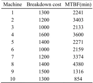
Table 5.3 Machine reliability information for example #2...86

Table 5.4 Similarity matrix for machines in example #2 ...86

Table 5.5 Formation of machine cells for numerical example #2 ...87

Table 5.6 Part routing assignment for numerical example #2 ...88

Table 5.7 Flow matrix...91

Table 6.1 Test instances from the literature for standard CFP...95

Table 6.2 Parameters setting for HCFA-HSAM, HCFA-HWFAM, and HCFA-HTSM...96

Table 6.3 The computational results in the case where singletons are allowed (Lm=1) ...98

Table 6.4 The computational results in the case where singletons are not allowed (Lm=2)100 Table 6.5 Test instances for generalized CFP...102

Table 6.6 Parameters setting for HGCFA-HSAM, HGCFA-HWFAM, and HGCFA-HTSM ...103

Table 6.7 Comparisons of computation results for different cellular layout type ...105

Table 6.8 The computational results for our proposed algorithms (stage I) in the case where linear double-row layout (r=2) is considered ...106

Table 6.9 The computational results for our proposed algorithms (stage II) in the case where linear double-row layout (r=2) is considered ...107

Table 7.1 ANOVA for the effects of algorithm and PENC...109

Table 7.2 Paired T-test for the effects of mutation operator for HTSM ... 111

(10)

Table 7.4 Experimental testing scenarios ... 112

Table 7.5 ANOVA for the effects of evaporation, precipitation, and insertion-move ... 112

Table 7.6 ANOVA for the effects of tabu list size ... 113

Table A.1 Machine reliability information for test instance 2... 117

Table A.6 Machine reliability information for test instance 8...120

Table A.7 Production data of test instance 3 ...121

(11)

LIST OF FIGURES

Figure 1.1 The flow chart of research...5

Figure 2.1 Classification of the CF solution method...8

Figure 2.2 Pseudo-code for general simulated annealing algorithm (Kirkpatrick et al., 1983)...16

Figure 2.3 Pseudo-code for general TS algorithm...17

Figure 2.4 Pseudo-code for WFA algorithm...22

Figure 3.1 Rearrangement of rows and columns of matrix to create cells ...37

Figure 3.2 Cell formation with alternative process routings ...39

Figure 3.3 Cellular layout...40

Figure 3.4 Two typical cellular layouts: (a) linear single-row layout (r=1) (b) linear double-row layout (r=2) ...40

Figure 3.5 Two typical cellular layouts (NC=3)...41

Figure 3.6 An example for the affect of operation sequence...42

Figure 3.7 The framework of the proposed two-stage model for generalized CFP ...44

Figure 3.8 Intracellular part flows ...47

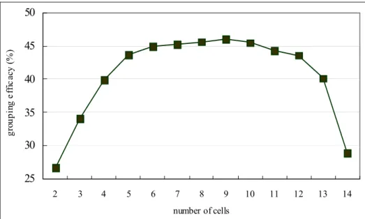
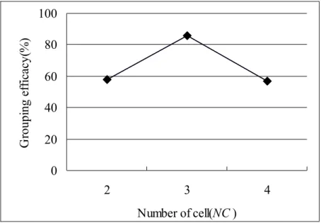
Figure 4.1 Relationship between grouping efficacy and number of cells ...52

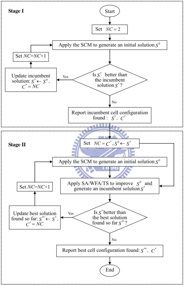
Figure 4.2 Two-stage approach: Hybrid Cell Formation Algorithm (HCFA) ...54

Figure 4.3 Machine-part matrix and corresponding similarity matrix for machines...56

Figure 4.4 Assignment of machines ...56

Figure 4.5 Initial solution matrix obtained ...57

Figure 4.6 Configuration of a feasible solution to the CFP...58

Figure 4.7 Pseudo code of mutation strategy ...59

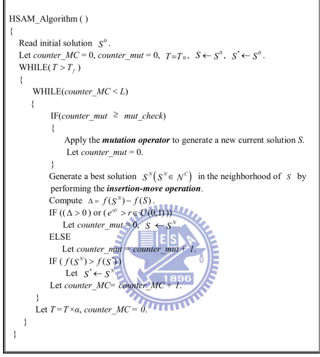
Figure 4.8 Pseudo code of proposed HSAM procedure ...62

(12)

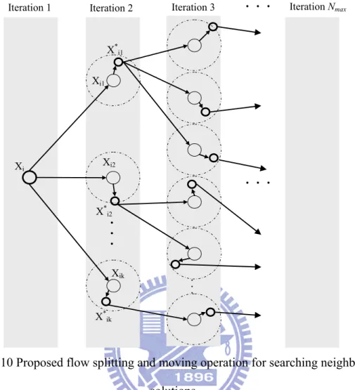
Figure 4.10 Proposed flow splitting and moving operation for searching neighborhood

solutions...67

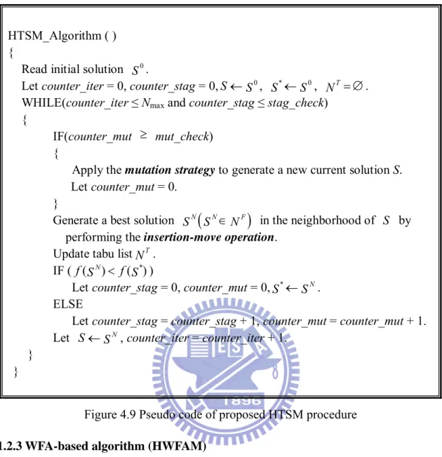
Figure 4.11 Pseudo code of proposed HWFAM procedure...70

Figure 4.12 Framework of the proposed hybrid generalized CF algorithm (HGCFA) ...71

Figure 4.13 Configuration of an initial solution to sequence of machines...77

Figure 4.14 Pseudo code of mutation strategy ...78

Figure 5.1 0-1 machine-part matrix of example #1...79

Figure 5.2 Assignment of machines ...81

Figure 5.3 Assignment of parts...82

Figure 5.4 Solution configuration for NC=2 ...82

Figure 5.5 Relationship between grouping efficacy and number of cells for example #1 ...83

Figure 5.6 Solution configuration for NC=3 ...83

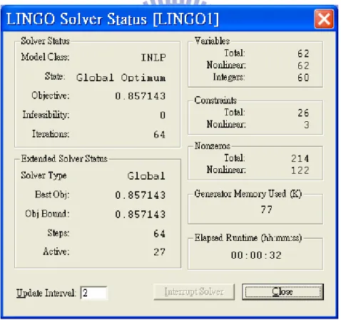
Figure 5.7 Lingo solver status for example #1 ...84

Figure 5.8 Initial linear single-row layout...86

Figure 5.9 Initial solution of stage I for example #2 ...89

Figure 5.10 Lingo solver status for stage I (cell formation and inter-cell layout)...90

Figure 5.11 Initial configuration of machine sequence for example #2 ...91

Figure 5.12 Final solution of stage II (cell formation, inter-cell layout and intra-cell layout)...92

Figure 5.13 Lingo solver status for stage II (intra-cell layout)...93

Figure 7.1 Mean CPU comparisons of with and without PENC ...109

Figure 7.2 The CPU time saving ratios of HTSM, HSAM, and HWFAM... 110

(13)

CHAPTER 1 INTRODUCTION

1.1 Research Motivations

In response to various and diversified customer demands, companies must adopt innovative manufacturing strategies and technologies to achieve an efficient and flexible manufacturing system. Group technology (GT) is one approach that meets the requirements of system flexibility and product variation. The cellular manufacturing system (CMS) is one of the applications of GT principles in manufacturing. Implementation of CMS resulted in significant benefits, such as reduced material handling costs, work-in-progress inventory, throughput and set-up times, simplified scheduling, and improved quality (Wemmerlov and Hyer, 1987). Hence, it has been widely discussed and applied by researchers and practitioners in the last three decades.

A cell formation problem (CFP) is the crucial element in designing a CMS (McAuley, 1972). However, the CFP in CMS is one of the NP-hard combinational problems (Kusiak, 1990). Hence, it is difficult to obtain optimal solutions in an acceptable length of time, especially for large-sized problems. Numerous models and solution approaches have been developed to address this problem since the 1970s. Different studies have focused on different aspects of CFP. Based on production data employed in CF models, the CFP is classified into two main categories: standard CFP represented by a binary machine-part incidence matrix and generalized CFP with more factors and system constraints considerations. Although many effective heuristics or algorithms have been done on standard CFP, very little has been devoted to integrate cell formation, cell layout, and intracellular machine layout, the three basic steps in the design of CMS, simultaneously with considerations of alternative process routings, operation sequences, production volume, and machine reliability on generalized CFP; thereby limiting the practical nature of their

(14)

approaches in a real CMS environment. Moreover, most methods in the literature assume that the NC is prescribed beforehand. However, determine the proper NC in the cell formation stage is very difficult for the layout designer because he does not have any knowledge at the beginning. Hence, it is important and more practical to integrate the abovementioned factors simultaneously in the design of CMS.

Due to their excellent performance in solving combinatorial optimization problems, meta-heuristic algorithms, such as simulated annealing (SA), water flow-like algorithm (WFA), and tabu search (TS), have been the most successful solution approach to provide global or near-global optimal solutions within a reasonable computation time. On the other hand, a number of similarity coefficient method (SCM)-based approaches have been proposed, and have been shown to produce good machine-part grouping and are more flexible in incorporating various production data into the machine-part clustering process.

Thus, the major research motivations for this thesis may be summarized as follows: (1) CMS may provide great benefits.

(2) CFP is the first and most difficult aspect of constructing a preliminary CMS. (3) CFP is one of the NP-hard combinational problems.

(4) There are few works that integrate cell formation, cell layout, and intracellular machine layout simultaneously with considerations of alternative process routings, operation sequences, production volume, production times, machine reliability, and different cellular layout type.

(5) It is difficult for a layout designer to determine the optimum cell number beforehand.

1.2 Research Objectives

Based on the research motivations, this thesis is dedicated to merging an SCM-based clustering algorithm and meta-heuristics to develop quick and effective hybrid algorithms to solve standard CFP and generalized CFP. Specific goals are as follows: (1) to merge an

(15)

SCM-based clustering algorithm and SA/TS/WFA method to present a fast and effective two-stage hybrid algorithm to solve standard CFP; (2) to formulate a two-stage multi-objective mathematical programming model to integrate cell formation, cell layout, and intracellular machine layout simultaneously with considerations of alternative process routings, operation sequences, production volume, machine reliability, and different cellular layout type; and (3) to integrate a generalized SCM-based clustering algorithm and SA/TS/WFA method to develop a fast and effective two-stage hybrid approach to resolve the formulated two-stage multi-objective mathematical programming model.

Unlike most previous studies where the NC to be formed is prescribed beforehand, the proposed methods do not demand a priori specification of the NC. Instead, it is automatically calculated and determined such that the best objective value may be achieved. Illustrative examples will be used to demonstrate the effectiveness of the proposed methods for standard CFP and generalized CFP. Hopefully, the proposed methods can be used to solve real CFP in factories by providing robust manufacturing cell formation in a short execution time.

1.3 Research Process

To achieve the abovementioned objectives, the research process (Figure 1.1) progresses as follows:

Step 1: Identifying research problems and objectives

Issues in CFP are identified through a discussion of research motivations and the purposes of this study.

Step 2: Literature review and discussion

The literature encompasses group technology and cellular manufacturing, solution methods for CFP, performance measures for CFP, and previous work on resolving CFP.

(16)

In this step, a mathematical model in terms of maximization of grouping efficacy is formulated to express standard CFP. Then, a two-stage multi-objective mathematical programming model for generalized CFP is formulated to integrate cell formation, cell layout, and intracellular machine layout simultaneously with considerations of alternative process routings, operation sequences, production volume, production times, machine reliability, and different cellular layout type.

Step 4: Development of proposed algorithms

In order to solve standard and generalized CFP mathematical models quickly and effectively, a two-stage hybrid CF algorithm (HCFA) merging an SCM-based clustering algorithm and SA/TS/WFA method is proposed to solve the standard CFP model. Afterwards, a two-stage hybrid generalized CF algorithm (HGCFA) merging a generalized SCM-based clustering algorithm and SA/TS/WFA method is proposed to solve the generalized CFP model.

Step 5: Validation of proposed algorithms

To demonstrate the power of our proposed algorithms for standard CFP, 35 test instances represented by a binary machine-part incidence matrix drawn from the literature are used to evaluate the computational characteristics of our proposed algorithms. On the other hand, 8 test instances, two drawn from the literature and the others prepared by adding self-creating data to test instances, are used to validate the quality of our proposed algorithm for generalized CFP.

Step 6: Summaries and Conclusions

(17)

Figure 1.1 The flow chart of research

1.4 Organization

The remaining chapters are organized as follows. We present a literature review of CFP and the requisite solution techniques, including SA, TS, and WFA in Chapter 2. The mathematical models that express standard CFP and generalized CFP are formulated in Chapter 3. In Chapter 4, two hybrid meta-heuristic algorithms based on SCM-based clustering algorithm and SA/TS/WFA are proposed to solve the complex models. In Chapter 5, two numerical illustrations are given to demonstrate the effectiveness of the proposed methods for standard CFP and generalized CFP. Computational results for standard CFP and generalized CFP are shown in Chapter 6. Several strategies proposed in this thesis, together with some mechanisms, are further analyzed in Chapter 7. Conclusions of this thesis are finally drawn in Chapter 8.

Identification of the problems and objectives of research The literature review and discussion

1. Group technology and Cellular Manufacturing 2. Solution Methods for CFP

3. Performance Measures for CFP 4. Previous Work on Resolving CFP

Formulation of mathematical models

Development of proposed algorithms

Summaries and conclusions Validation of proposed algorithms

(18)

CHAPTER 2 LITERATURE REVIEW

This chapter is divided into fours sections. Section 2.1 introduces and defines GT and CM. Cell formation methods are reviewed in Section 2.2, while Section 2.3 describes the performance measures for CFP. Section 2.4 provides a review of previous work on resolving CFP.

2.1 Group Technology and Cellular Manufacturing

GT was originally introduced by Mitrovanov (1966) and was popularized in the west by Burbidge (1975). One application of GT is CM, a manufacturing philosophy in which similar parts are identified and grouped into part families, while machines are grouped into machine cells to take advantage of their similarities in manufacturing and design. Implementation of CM results in significant benefits, such as reduced material handling costs, work-in-progress inventory, throughput and set-up times, simplified scheduling, and improved quality (Wemmerlov and Hyer, 1987).

Although CM may provide great benefits, the CMS design is complex for real life problems. The design of a CMS consists of four stages as described below (Wemmerlov and Hyer, 1986).

1. CF – grouping parts with similar design features or processing requirements into part families and associated machines into machine cells.

2. Group layout – laying out machines within each cell (intra-cell layout) and cells with respect to one another (inter-cell layout).

3. Group scheduling – scheduling parts and part families for production. 4. Resource allocation – assigning tools, human and material resources.

Ideally, all of these stages should be addressed simultaneously in order to obtain the best results (Alfa et al., 1992). However, due to the complex nature of each stage and the

(19)

limitations of traditional approaches, this thesis will focus on stages 1 and 2. The solution methods for stages 1 and 2 will be discussed in the next section.

2.2 Solution Methods for CFP

The process of determining part families and machine groups is referred to as the CFP. It is known that the CFP in CMS is one of the NP-hard combinational problems (Ballakur and Steudel, 1987). Numerous solution approaches have been developed to address CFP since the 1970s, and these can be classified into five categories (Figure 2.1): (1) array-based methods, (2) similarity coefficient methods, (3) graph theoretic methods (4) mathematical programming methods, and (5) heuristic and meta-heuristic methods. Similarity coefficient methods and heuristic and meta-heuristic methods are related to this research and are discussed further.

(1) Array-based methods

The array-based methods attempt to allocate machines into groups and parts into associated families by appropriately rearranging the order of rows and columns to find a block diagonal form of the aki = 1 entries in the machine-part incidence matrix. The

machine-part incidence matrix has 0 and 1 entries (aki). A ‘1’ entry in row k and column i of

the matrix indicates that part i has an operation on machine k, whereas a ‘0’ entry indicates that it does not. Although cluster analysis methodologies are simple to implement, they have one main drawback: it usually takes into account only one objective i.e. the minimization of intercellular movements where only part operations and the machines involved are considered. Other product data (such as operational sequences and processing times) are not incorporated into the design process. Thus, solutions obtained may be valid for limited situations only.

(20)

Figure 2.1 Classification of the CF solution method Cell Formation Methods Similarity coefficient Graph partitioning Mathematical programming Heuristic and metaheuristic Hierarchical Non-hierarchical SA TS GA LP DP GP LQP ACO PSO ANN Array-based WFA

(21)

(2) Graph theoretic methods

In graph partitioning approaches, the process of forming manufacturing cells starts with collecting problem data and then converting them into a weighted network diagram. Finally, the weighted network diagram is separated into several sub-groups of a machine cell. In the network diagram, nodes represent machines and arcs represent their relationships, defined as the value of total part flow between machines. In this method, the network diagram can clearly depict the flow of the machine, but other product data (such as machine capacity, processing times) are not easily incorporated. Therefore, graph partitioning approaches do not directly show the characteristics of multi-objective cell design.

(3) Mathematical programming methods

Mathematical programming methods can be presented in two parts: objective function and constraints. The establishment of objective function usually considers the factors related to manufacturing, e.g. minimizing inter-cell movement of parts, minimizing cell load unbalances, minimizing number of exceptional, and minimizing total manufacturing cost. Constraints express the content of production conditions, such as the limitation on number of machines, number of jobs, utilized time of tools, cells of machine allocation, controller’s work time, and capability limitation. Mathematical programming methods can be further classified into four major groups based on the type of formulation: (1) linear programming (LP), (2) linear and quadratic integer programming (LQP), (3) dynamic programming (DP), and (4) goal programming (GP). The greatest advantage of this method is that different design objectives and constraints can be incorporated into a single formulated model. However, NP completeness of the problems makes it computationally intractable, especially for large-sized problems.

2.2.1 Similarity Coefficient Methods

(22)

SCM are more flexible in incorporating various production data into the machine-part clustering process (Seifoddini and Tjahjana, 1999). The solution procedure of SCM usually follows a prescribed set of steps (Romesburg, 1984), the main ones being: (1) getting input data, (2) calculating the similarity coefficient, and (3) selecting a clustering algorithm to get machine cells. These steps are described next.

(1) Getting input data

Input data can be obtained from routing cards. These information are usually represented in a matrix called the machine-part incidence matrix, which is an m × p matrix with 0 or 1 entry, where m is the number of machines and p is the number of parts. Rows represent the machines and columns represent the parts. An element aij of the matrix is 1 if

the jth part visits the ith machine for processing; otherwise, the value is 0. (2) Calculating the similarity coefficient

The similarity coefficient is defined as a measure of similarity between machines, tools, design features, and so forth. Yin and Yasuda (2005) evaluated the performance of 20 well-known similarity coefficients, and found that the Jaccard similarity coefficient (Jaccard, 1908) is the most stable similarity coefficient. For this reason, we use the Jaccard similarity coefficient and the generalized similarity coefficient (Won and Kim, 1997) to calculate the similarity coefficient of standard CFP and generalized CFP, respectively. The generalized similarity coefficient is an extension of the Jaccard similarity coefficient (McAuley, 1972) and has been proposed for considering alternative process plans.

The Jaccard similarity coefficient is defined as the ratio of the number of parts visiting both machines and the number of parts visiting one of the two machines:

ij ij ij ij ij a S a b c = + + (2.1)

where aij represents the number of parts processed by both machines i and j; while bij is

(23)

parts processed by machine j but not by machine i.

On the other hand, the generalized similarity coefficient is formulated as:

ij ij i j ij N S N N N = + − (2.2) where

Sij = similarity coefficient between machines i and j

1 , 1 , 1 p p p k k k i i j j ij ij k k k N a N a N a = = = =∑ =∑ =∑ p = number of parts

1 if some routing of part 0 otherwise

1 if , some routing of part synchronously 0 otherwise k i k j k ij i k j k i j k a a a ∈ ⎧ = ⎨ ⎩ ∈ ⎧ = ⎨ ⎩ ∈ ⎧ = ⎨ ⎩

(3) Selecting a clustering algorithm to get machine cells

When the values of the similarity coefficients have been calculated, a clustering algorithm can be selected to get machine cells. Conventional clustering algorithms are divided into two major classes: hierarchical and non-hierarchical. Hierarchical clustering for CF comprises two stages. Initially, some form of similarity or dissimilarity between machines or parts is employed in order to create machine cells or part families. Later, machines or parts are separated into a few broad cells, each of which is further divided into smaller groups and each of these further partitioned and so on until terminal groups that cannot be subdivided are generated. Essentially, hierarchical techniques can be classified into two: (a) divisive methods where the process starts with all the data (machines or parts) in a single group and a series of partitions is created until each machine (part) is in a singleton cluster and, (b) agglomerative methods where the process starts with singleton

(24)

whole set is obtained.

Non-hierarchical clustering methods are iterative methods that also employ a measure of similarity or dissimilarity for grouping parts or machines. They begin with either an initial partition of the data set or the choice of a few seed points. In either case, the number of clusters has to be decided on beforehand.

Among the abovementioned approaches, the SCMs are more flexible in incorporating various production data into the machine-part clustering process. On the other hand, the heuristic and meta-heuristic methods are especially useful in providing near-optimum solutions within a reasonable computation time when a CFP cannot be solved using traditional methods, and thus constitute the state-of-the-art algorithm for solving CFP.

2.2.2 Heuristic and meta-heuristic methods

Heuristic and meta-heuristic methods are random heuristic search algorithms applicable to a wide variety of combinatorial optimization problems. They include SA (Su and Hsu 1998, Sofianopoulou 1999, Arkat et al. 2007), TS (Sun et al. 1995, Adenso-Diaz et

al. 2001, Wu et al. 2004, Lei and Wu 2005), genetic algorithms (GA; Lee et al. 1997,

Onwubolu and Mutingi 2001, Boulif and Atif 2006, Chan et al. 2008), ant colony optimization (ACO; Kao and Fu 2006), particle swarm optimization (PSO; Andres and Lozano 2006), artificial neural network (ANN; Park and Suresh 2003, Yang and Yang 2008), and WFA (Yang and Wang 2007). Although heuristic and meta-heuristic methods are not guaranteed to provide optimal solutions (they usually give sub-optimal results), they are very useful in producing acceptable solutions within a reasonable time. In fact, optimal results can only be obtained under very restricted conditions; this makes heuristic and meta-heuristic methods more practical in real-life applications. SA, TS, and WFA are relevant to this research and are discussed further.

(25)

2.2.2.1 Simulated Annealing

SA algorithm was originally proposed by Metropolis et al. (1953) to simulate the annealing process. Based on this pioneering work, Kirkpatrick et al. (1983) first introduced the general optimization algorithm of SA to solve hard combinatorial optimization problems through controlled randomization. Lundy and Mees (1986) proved that the SA algorithm converges to the global optimum with a probability close to one under certain assumptions. SA poses several advantages over other sophisticated combinatorial optimization approaches, e.g. relatively easy and quick implementation, flexibility, and transparency. Due to its ease of use and its ability to provide a good solution for real-world problems, SA is one of the most powerful and popular heuristics to solve many optimization problems. For instance, adequate results have been attained when applying SA on various combinatorial problems (Kirkpatrick et al. 1983, Bonomi and Lutton 1984, Aarts and Van Laarhoven 1985, Selim and Alsultan 1991, Mckendall et al. 2006, Yu et al. 2010).

The pseudo-code of the general procedure for implementing the SA algorithm in maximization problems is presented in Figure 2.2. The algorithm starts with a high temperature. After generating an initial solution (S0), it attempts to move from the current solution (S) to one of its neighborhood solutions (_SN_{).Changes in objective function values}

(Δ=_SN_{-S) are computed. The new solution is accepted if it results in better objective value}

(i.e. Δ>0). However, if the new solution yields worse value, it can still be accepted according to the probability function p₌eΔT_{, where T is the current temperature. This}

check is performed by first selecting a random number (r) from (0, 1). If the value is less than or equal to the probability value (p), the new configuration is accepted; otherwise, it is rejected. By accepting worse solutions, SA can avoid being trapped on local optima. SA repeats this process L times at each temperature to reach the thermal equilibrium, where L is a control parameter usually called the Markov chain length or Epoch length. The parameter

(26)

T is gradually decreased by a cooling function as SA proceeds until the stopping condition

is met.

The general scheme of SA can be stated as follows: Step 1. Choose an initial temperature T.

Step 2. Generate a random candidate S.

Step 3. If a stopping criterion is satisfied, then stop; otherwise repeat the following steps: Step 3.1. If “thermal equilibrium is reached,” then exit this loop.

Step 3.2. Let _SN_{be a randomly selected neighbor of S.}

Step 3.3. Generate a uniform random number r from [0, 1].

Step 3.4. Compute the changes in the objective function values: ( N )

S S

Δ = − .

Step 3.5. If _eΔT > , then _r N

S S= .

Step 4. Let T be a new (lower) temperature value, then go to Step 3.

The annealing schedule mainly consists of (1) the initial temperature, (2) a cooling function, (3) the number of iterations to be performed at each temperature, and (4) a stopping criterion to terminate the algorithm. Performance analysis of SA had revealed several characteristics (Lin et al., 1993):

(1) There is a tradeoff between the quality of the final solution obtained and the execution time required. Furthermore, the execution time is sensitive to the decrement ratio of the temperature.

(2) If the temperature drops too sharply, is the algorithm becomes easily trapped in local minima.

(3) Detecting the equilibrium of the system at each temperature level is not an easy task. (4) The total number of iterations of SA is affected by the initial temperature.

(5) If the numbers of iterations at low temperature regions are not large enough, there are still some probability of departing from good solutions.

(27)

algorithm described above. These include the following:

(1) Choice of an initial temperature and the corresponding temperature decrement strategy At a high temperature, almost all unimproved trial solutions are accepted. However, at a lower temperature, fewer unimproved trial solutions can be accepted. If the cooling speed is too fast or the initial temperature (T0) is not high enough, this mechanism will fail

to escape local minima. T0 should be high enough that in the first iteration of the algorithm,

the probability of accepting worst solutions is, at least, 80% (Kirkpatrick et al., 1983). The most commonly used temperature decrement function is geometric: T =a× T, where a< 1 and constant. Typically, 0.7 ≤ a≤ 0.95.

(2) Choice of a criterion for detecting equilibrium

For each value of the current temperature T, the inner loop (steps 3.1 to 3.5 in the algorithm presented above) should be repeated L times in order for the system to reach “thermal equilibrium.” If the search cannot reach the equilibrium state at each temperature, obtaining a globally optimum solution becomes difficult. A good criterion for thermal equilibrium can save computational effort without losing the ability of escaping from a local minimum.

(3) Choice of an adequate stopping criterion

The stopping criterion is used to stop the algorithm when there is sufficient evidence that the global optimum has been detected or that the “cost” connected with the search for a better estimate of the global optimum would be too high. The stop can also occur when some kind of “resource” has been exhausted, e.g. computer time, the total number of solutions generated, and when the desired energy level is attained (freezing temperature). The stopping criterion is always the crucial and most difficult part of the algorithm, and has great influence on overall performance.

(28)

to be defined when adopting this general algorithm to a specific problem are the procedures to generate both the initial solution and the neighboring solutions. The details of the proposed implementation of the SA to the CFP are presented in Section 4.1.2.

SA_Algorithm ( ) {

Generate an initial solution 0

S .

Let the current solution S equal to 0

S .

Let the current best solution *

S equal toS . 0

Let the current temperature T equal to the initial temperature T0.

WHILE(stop criterion is false) // outer loop {

Let repetition counter n = 1.

WHILE(n < Markov chain length L) // inner loop {

Generate a random solution N

S in the neighborhood of S. Compute Δ= _f( N) _{f S}( ) S − . IF (Δ>0 or T (0,1) eΔ _{> ∈}r U ) Let N S ←S . IF ( _f₍ N₎ _f_{( )}* S > S ) Let * N S ←S . n= n + 1. }

Reduce the temperature T. }

}

Figure 2.2 Pseudo-code for general simulated annealing algorithm (Kirkpatrick et al., 1983) 2.2.2.2 Tabu Search

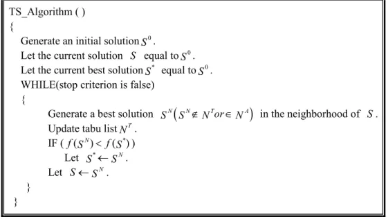
TS is a meta-heuristic approach designed to find optimal or near-optimal solutions to combinatorial optimization problems. This method has been suggested primarily by Glover

et al. (1985) and further refined and developed by Glover (1986, 1989, and 1990). The

(29)

TS_Algorithm ( ) {

Generate an initial solution 0

S .

Let the current solution S equal to 0

S .

Let the current best solution *

S equal toS . 0

WHILE(stop criterion is false) {

Generate a best solution _SN

(

_SN_∉_NT_or_∈_NA

)

_{in the neighborhood of S .} Update tabu list_{N .}T

IF ( _f₍_SN₎_< _f_{( )}_S* ₎

Let _S*_←_SN_. Let _S_←_SN_. }

}

Figure 2.3 Pseudo-code for general TS algorithm

The algorithm begins from a randomly selected or a known initial solution ( 0

S ). From

this solution, a set of neighborhood solutions of the current solution (S) is generated using

the predefined movement strategies. The objective function is evaluated for each neighborhood of S and the best neighbor solution (_{S ) replaces the S even though the best}N

neighbor solution may be worse than the current one. In this way, the algorithm can escape from the local minima (or maxima) of the objective function. However, the algorithm may recycle. To avoid this situation, certain attributes of the last replaced solution are stored in a list, which is called a tabu list ( T

N ). The neighbors of S that satisfy conditions given by the

tabu list are systematically eliminated unless they meet an aspiration criterion ( A

N ), so that

at each iteration, the algorithm is forced to select a point not recently selected. TS has been successfully used to solve many optimization problems in a wide variety of areas, including CFP, graph coloring, traveling salesman problem, path assignment, flow shop sequencing, job shop sequencing, and dealing with learning in neural networks (Glover and Languna, 1993). More detailed discussions of the foundations of TS methodology can be found in Glover (1989, 1990) and Glover and Laguna (1997).

(30)

moves, tabu list, aspiration criterion, stopping criterion, intensification, and diversification. The details of these are described next.

(1) Initial solution

The quality of the initial solution is crucial to the efficiency of TS. It is known that a good initial solution will improve the efficiency of TS. Generally, the initial solution is produced by some rules or problem-specific heuristics instead of random generation.

(2) Neighborhood and moves

The neighborhood of a solution is the set of all formations that can be arrived at by a move. Since neighborhood depends on the current solution, new neighborhood is generated every time the current solution changes. Generally, neighboring solutions can be generated by insertion method, pair-wise interchange, and adjacent interchange method. Different methods are employed according to the problem. From all neighboring solutions, the best one is chosen to move forward. However, this best solution may sometimes be in the tabu list and does not satisfy aspiration criterion. When this happens, the second best solution is chosen to move forward if it is not in the tabu list; otherwise, the third best solution is considered and so on.

(3) Tabu list

In order to prevent scheme cycling and returning to the same solutions, it is necessary to introduce a condition that prevents this from happening. This is usually carried out by not allowing reversal of moves for a certain number of iterations equal to the tabu length. These non-admissible moves within the short interval comprise the class membership of a tabu list. The size of the tabu list must be large enough to prevent cycling, but small enough to not forbid too many moves. A minimum of 7 and a maximum of 11 has been suggested for tabu length (Glover and Laguna, 1993).

(4) Aspiration criterion

(31)

better than the best solution found thus far. Thus, if a tabu move satisfies the associated aspiration criterion, it is considered admissible.

(5) Stopping criterion

The most accepted stopping criterion relies on the search being terminated if the objective function value has not improved within a certain number of iterations that is usually specified at the start of the run. Another criterion relies on the search being terminated if a maximum number of iterations has been reached to avoid an extremely long run. The problem with the latter criterion is that it is difficult to determine the maximum number of iterations because the value may either lead to premature termination or expensive termination.

(6) Intensification

The mechanism for intensification enhances the search to focus on examining elite solutions in a neighborhood. It tends to move the search to a neighboring position in the search space, and so could be considered a local search.

(7) Diversification

The mechanism for diversification allows a large jump to be made in the solution space. This ensures that large areas of the space are searched and solutions do not get stuck in local minima. This mechanism is also referred to as the restarting procedure. For each diversification process, a different initial cell formation is randomly generated. This way, the search is able to explore a large solution space, thereby enhancing the possibility of finding the optimum solution in a very short time.

TS has the following characteristics:

(1) Utilizes a flexible memory structure, which is more efficient than strict memory structure (ex: branch-and-bound) or no memory (ex: simulated annealing).

(32)

(4) Updates the tabu list in every step to reduce the probability of redundant searching and to improve searching efficiency.

(5) Uses an aspiration criterion to relax tabu restriction and keep the searching process going. (6) Sets upper bounds of iteration numbers passed or time elapsed to terminate the searching

process.

2.2.2.3 Water Flow-like Algorithm

The design of the WFA (Yang and Wang, 2007) was inspired by the natural behavior of water flowing from higher to lower levels. On the earth’s surface, a flow will split into multiple sub-flows when rugged terrains are traversed. Sub-flows, however, will merge when they arrive at the same location. Governed by gravity and driven by fluid momentum, flows can run to higher levels or run over bumps to navigate various terrains. Water flow will cease and stagnate at the locally or globally lowest depression; when the momentum left cannot expel the water out of the depression, it will stagnate at its current location. No movement is allowed until other flows merge with it or until the water evaporates into the atmosphere. When the evaporated water accumulates to some extent, it will return to the ground as several new downpour flows, such that rainfall occurs occasionally. As the solution space of a problem can be mapped to the geographical terrain, and the objective value is mapped to the altitude, each flow can then be regarded as a solution agent. Water moving to a lower position can be considered as a solution searching for the optima. Thus, the solution search process has been modeled as water flow.

Yang and Wang (2007) adopted several natural behaviors of water flow in presenting the WFA (Dougherty and Marryott, 1991). Their design ideas are summarized as follows: (1) Driven by gravity and governed by the energy conservation law, water will constantly

flow to lower altitudes. Conversely, the solution search will recursively move from inferior to superior solutions.

(33)

(2) Fluid momentum drives water forward through rough terrains. A flow will split into sub-flows when it encounters rugged terrain and when its momentum exceeds a base amount for splitting. WFA simulates this behavior as an agent forking operation; that is, more than two agents are derived from a single agent. A flow with larger momentum will generate more streams of sub-flows than one with less momentum. A flow with limited momentum will yield to the landform and maintain a single flow. Therefore, the fluid momentum of a flow is recalculated to determine the number of sub-flows that can be forked after each move.

(3) Water flows to lower altitudes and occasionally swells to higher altitudes as long as the kinetic energy is larger than the required potential energy. To avoid being trapped within a local minimum, WFA allows the water to flow to a worse location to broaden the exploration area, provided it has enough kinetic energy.

(4) A number of flows merge into a single flow when they meet at the same location. WFA reduces the number of solution agents when multiple agents result in the same objective value to avoid redundant searches.

(5) Water flows are subject to water evaporation in the atmosphere. The evaporated water will return to the ground in the form of rainfall. In WFA, a part of the water flow is manually removed to mimic water evaporation. After evaporation, a precipitation operation is implemented in WFA to simulate natural rainfall and explore a wider solution area.

The pseudo-code for the general procedure for implementing the WFA is shown in Figure 2.4.

(34)

WFA_Algorithm ( ) {

Generate an initial solution. WHILE(stop criterion is false) {

Flow splitting and moving. Flow merging. Water evaporation. IF (rainfall required) { Precipitation. Flow Merging. }

IF (new best solution found) Update best solution record. }

}

Figure 2.4 Pseudo-code for WFA algorithm

The WFA algorithm consists of four primary operations: (1) flow splitting and moving, (2) flow merging, (3) water evaporation, and (4) precipitation. Before proceeding to the descriptions of these four operations, we introduce some notations.

Nmax : Iteration limit

W0 : Initial mass of original flow

Wi : Mass of flow i

V0 : Initial velocity of original flow

Vi : Velocity of flow i

Tm : Base momentum

n : Upper limit on number of subflows split from a flow

ni : Number of subflows forked from flow i

N : Total number of water flows in current iteration

ik

(35)

ik

δ : Attitude drop from flow i to subflow k; equivalently, changes in objective value

from solution i to its neighborhood solution k

G : Gravitational acceleration

T : A prescribed number of iteration a flow will be removed by evaporation

1. Flow splitting and moving operation

It is assumed that there is only one water flow in the beginning of the WFA, and that its location is randomly generated. Driven by fluid momentum and potential energy, the flow starts to move to new locations to explore the solution space for new and better solutions. Yang and Wang (2007) used constant-step movement to the best neighborhood solution when solving the object grouping problem. However, various flow-moving strategies can be designed and applied depending on the characteristics of different optimization problems.

In the WFA, flow splitting results from capable momentum, and a flow with higher momentum generates more sub-flows than that with a lower one. The locations of the split sub-flows are derived from the neighboring locations of the original flow. When a flow does not split, it goes on as a single stream to the best feasible neighboring location. Allowing N to be the number of water flows in the current iteration, the number of sub-flows ni forked

from flow i (i = 1, 2, …, N) is determined by its momentum, WiVi. A flow with zero

momentum stays in its current location and is considered a stagnant solution. A flow can split into sub-flows only when its momentum exceeds a predefined base momentum Tm. The

number of sub-flows is determined by dividing its momentum by the base momentum Tm. If

the momentum of a flow is between 0 and Tm, it is treated as a single stream moving to a

new location without splitting. As WFA proceeds, it is possible that the number of sub-flows grows exponentially and exhausts the computational resource. Yang and Wang (2007) suggests imposing an upper limit n on the number of sub-flows forked from a flow at each iteration. The number of sub-flows split from a flow can thus be obtained through:

(36)

min max 1, int i i , i m WV n n T ⎧ ⎧ ⎛ ⎞⎫ ⎫ ⎪ ⎪ = _⎨ _⎨ _⎜ _⎟_⎬ _⎬ ⎝ ⎠ ⎪ ⎩ ⎭ ⎪ ⎩ ⎭ (2.8)

When the flow is split into sub-flows, its original mass has to be accordingly distributed to sub-flows based on the rule designed. Yang and Wang (2007) distributed mass based on the ranks of the sub-flows, as shown in Eq. (2.9).

1 1 , 1, 2,..., i i ik n i i r n k w W k n r = ⎛ ⎞ + − ⎜ ⎟ =_⎜ _⎟ = ⎜ ⎟ ⎝ ∑ ⎠ (2.9)

For instance, if Wi =5 and ni =3, then

1 2 1 3 2 1 5, 5, 5. 1 2 3 1 2 3 1 2 3 i i i w =_⎜⎛ ⎞_⎟ w =⎛_⎜ ⎞_⎟ w =⎛_⎜ ⎞_⎟ + + + + + + ⎝ ⎠ ⎝ ⎠ ⎝ ⎠

The velocity of each sub-flow is computed from the equation of energy conservation.

ik

μ , the velocity of sub-flow k split from flow i, is:

2 ₂ _, 2 ₂ ₀ 0 , i ik i ik ik g if g V V otherwise δ δ μ = ⎨⎧⎪ + + > ⎪⎩ (2.10)

where g is the gravitational acceleration, and δ_ik is the altitude drop from flow i to its sub-flow k; that is, the improvement of objective value moving from current solution i to its neighborhood solution k. When 2 ₂

i ik

V + gδ < 0, the momentum delivered to sub-flow k has been used up, implying that this sub-flow will stagnate in its current location (e.g. the solution is trapped in local optima) without splitting and movement. Such stagnant flow will gradually evaporate into the atmosphere, returning to the ground by precipitation later on.

At the end of the splitting and moving operation, the original flow becomes discarded because sub-flows have been generated. Information regarding the current number of sub-flows and solutions sets will then be recorded.

2. Flow-merging operation

(37)

with a bigger mass and momentum. Whether a flow shares the same location with others in the WFA is thus systematically examined. If a flow does share the same location, the latter flow is then merged into the former one. Assuming that flows i and j share the same location, then flow j will be deleted and the mass and velocity of flow i will be updated as follows:

i i j W =W W+ _(2.11) i i j j i i j WV W V V W W + = + (2.12)

Using the flow-merging operation, the WFA reduces the number of solution agents when multiple agents result in the same objective value in order to avoid redundant searches.

3. Water evaporation operation

It is natural for water to evaporate and return to the ground through precipitation after possible movement from its original location. Water evaporation and precipitation coincide with the “escaping from local optima” mechanism that many heuristic algorithms nowadays use to avoid being trapped and to explore more solution spaces.

Each flow in the WFA is subject to water evaporation, where part of the water evaporates into the atmosphere. It is determined that a flow will be completely removed after a prescribed number of iterations t; that is, the masses of all flows are decreased by the ratio of 1/t, as shown in Eq. (2.13), every time evaporation occurs.

1 1 , 1, 2,..., i i W W i N t ⎛ ⎞ = −_⎜ _⎟ = ⎝ ⎠ (2.13) 4. Precipitation operation

When water vapor accumulates to a certain volume, it will return to the ground in some form such as rain. In the original WFA, two types of precipitation are performed to simulate the natural cycle of water: enforced and regular precipitation.

(38)

Enforced precipitation is applied when all flows are grounded with zero velocities. Under this circumstance, all flows are forced to evaporate into the atmosphere and then returned to the ground without changing the number of current flows. However, the locations of these returned flows are deviated stochastically from the original ones. Mass of

W0 is proportionally distributed to flows based on their original mass with the same initial

velocity. Consequently, the mass assigned to flow i, W’i, can be determined using Eq. (2.14).

' 0 1 i i N k k W W W W = ⎛ ⎞ ⎜ ⎟ = ⎜ ⎟ ⎜ ⎟ ⎝∑ ⎠ (2.14)

Regular precipitation is applied periodically in balance with water evaporation. The regular precipitation operation is performed every t (same t value as in evaporation) iterations to pour down the evaporated water. Note that the cumulative mass of the evaporated water is ₀ 1 N k k W W =

−∑ . Thus, instead of using Eq. (2.14), the mass assigned to flow

i, W’i, is determined using Eq. (2.15) when applying regular precipitation. The newly poured

flow joins the current solution set, thus increasing the number of current solutions. In addition, both enforced and regular precipitation might generate several new flows in the same locations. A flow merging operation will be executed to eliminate possible redundant flows.

(

)

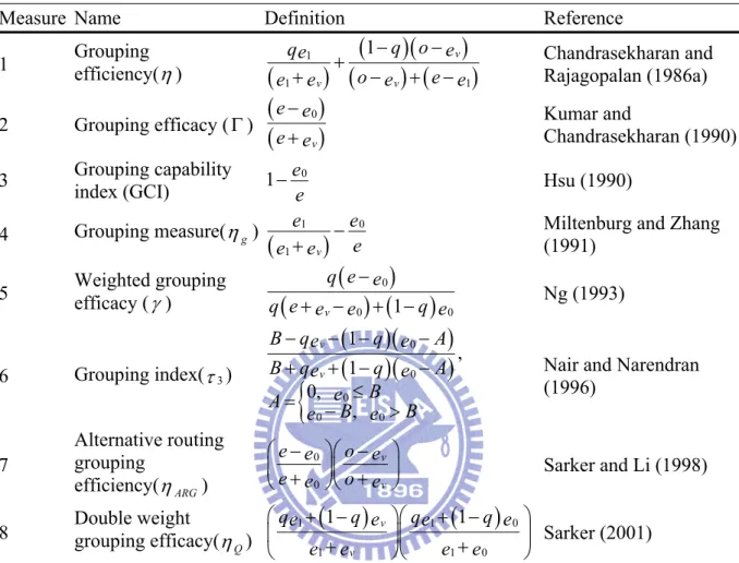
' 0 1 1 N i i N k k k k W W W W _W = = = −∑ ∑ (2.15)

2.3 Performance Measures for CFP

There is a need to develop performance measures or criteria in order to compare the quality of solutions obtained by different methods on an absolute scale. A limited number of performance measures have been proposed. Some commonly known grouping efficiency measures for 0-1 machine-part incidence matrix data are illustrated in Table 2.1. Among

(39)

them, two measures frequently used are the grouping efficiency (Chandrashekharan and Rajagopalan, 1987) and the grouping efficacy (Kumar and Chandrasekharan, 1990) because of their ease of implementation.

Although grouping efficiency has been used widely, critics argue that it has weak discriminating power (i.e., the ability to distinguish good quality grouping from bad). For example, a bad solution with large number of exceptional elements will give a value around 0.75. To overcome the low discriminating power of grouping efficiency between well-structured and ill-structured incidence matrices, Kumar and Chandrasekharan (1990) proposed another measure that they called grouping efficacy. Unlike grouping efficiency, grouping efficacy is not affected by the size of the matrix. Today, grouping efficacy is one of the most widely used measures applied to the CFP when a binary machine-part incidence matrix is used. Grouping efficacy can be defined as:

v e e e e + − = Γ 0 _, (2.3) where e is the total number of 1s in the matrix; e₀ is the total number of exceptional elements; and e_v is the total number of voids. Those 1’s outside the diagonal blocks are called ‘‘exceptional elements’’, while those 0’s inside the diagonal blocks are called ‘‘voids.” Grouping efficacy ranges from 0 to 1, with 1 being the perfect grouping.

We chose grouping efficacy as the measure of performance for the standard CFP in this thesis for several reasons:

(1) In the literature, it has been considered the standard measure to report the quality of the grouping solutions.

(2) It has a high capability to differentiate between well-structured and ill-structured matrices (e.g. high discriminating power).

(3) It is considered a better measure than grouping efficiency.

(40)

(5) It generates block diagonal matrices that are attractive in practice. (6) It does not require a weighting factor.

Table 2.1 Commonly known measures for 0-1 machine-part incidence matrix data

Measure Name Definition Reference

1 Grouping _efficiency(_η₎

₍

1

₎

₍

(

_{) (}

)(

)

₎

1 1 1 v v v q o qe e o e e e e e − − +

+ − + − Chandrasekharan and Rajagopalan (1986a) 2 Grouping efficacy (Γ )

(

₍

0

)

₎

v

e e e e

−

+ Kumar and Chandrasekharan (1990)

3 Grouping capability _{index (GCI)} _{1 e}0 e − Hsu (1990) 4 Grouping measure(ηg)

(

)

1 0 1 v e e e e +e −

Miltenburg and Zhang (1991)

5 Weighted grouping _{efficacy (}_γ ₎

₍

(

_{) (}

0

)

₎

0 1 0 v q e e q e e e q e − + − + − Ng (1993) 6 Grouping index(τ3)

(

)(

)

(

)(

)

{

0 0 0 0 0 1 , 1 0, , v v B qe q e A B qe q e A B e A _B _B e e − − − − + + − − ≤ = ₋ _>

Nair and Narendran (1996) 7 Alternative routing grouping efficiency(η_ARG) 0 0 v v e e o e e e o e ⎛ − ⎞⎛ − ⎞ ⎜ ₊ ⎟⎜ ₊ ⎟ ⎝ ⎠⎝ ⎠ Sarker and Li (1998)

8 Double weight _{grouping efficacy(}

Q η ) 1

(

)

1

(

)

0 1 1 0 1 v 1 v qe q e qe q e e e e e ⎛ + − ⎞⎛ + − ⎞ ⎜ ₊ ⎟⎜ ₊ ⎟ ⎝ ⎠⎝ ⎠ Sarker (2001)

e: total number of ones in the machine-part incidence matrix; o: total number of zeros in the machine-part

incidence matrix; e0: total number of exceptional elements; ev: total number of voids; e1: total number of ones within the diagonal blocks; q: weighting factor.

Although grouping efficiency and grouping efficacy have been used widely, they do not consider production factors, such as process sequence of operations, production volumes processing times of operations, and were designed for 0–1 matrices only. Hence, Harhalakis et al. (1990) proposed another measure called the group technology efficiency (GTE) that takes into account the sequence of operation, which can be defined as:

GTE=1 U

I

− , (2.4)

where I is the maximum number of inter-cell travels possible and U is the number of inter-cell travels actually required by the system.

(41)

Seifoddini and Djassimi (1995) developed a new grouping measure called Quality Index (QI) that takes into account the sequence of operation, production volume, and processing times of operation. This can be defined as:

Quality Index (QI ) =1 ICW

PW

− , (2.5)

where ICW is the intercellular workload and PW is the total plant’s workload.

Nair and Narendran (1998) observed that the GTE is inadequate because it is poor in pattern recognition. Hence, they proposed another measure called bond efficiency that takes into account inter-cell moves within cells and compactness, which can be defined as:

Bond efficiency(BE) =q GTE× + − ×

(

1 q

)

Compactness, (2.6) where q

(

0≤ ≤q 1

)

is a weighting factor; and Compactness is the ratio of the number of operations within it to the maximum number of operations possible in it, and is given by:

Compactness=

(

1

)

1 NC k k NC k k k TOTOP TOTOP NOP = = ∑ + ∑ , (2.7)

where NC is the maximum number of machine-cells; TOTOPk is the total number of

operations in the kth cell；and NOPk is the total number of non-operations (voids) in the kth

cell.

Although the abovementioned performance measures have taken into account the production sequence, production volume, and processing times of operation, many realistic factors such as alternative process routings, cellular layout, and machine reliability are still not considered simultaneously. If incorporated, these factors can enhance the quality of solutions. Hence, a performance measure for cell formation, cell layout, and intracellular machine layout with considerations of alternative process routings, operation sequences, production volume, machine reliability, and different cellular layout type is developed in Section 3.4.

(42)

2.4 Previous Work on Resolving CFP

Numerous models and solution approaches have been developed to deal with CFP since the 1970s. Some focus on developing effective heuristics or algorithms for solving standard CFP in which machine cells and part families are obtained sequentially or simultaneously. For instance, McAuley (1972) and Carrie (1973) developed the first algorithms using SCM on CFP. King and Nakornchai (1982) developed the earliest array-based methods to solve CFP. Cheng et al. (1998) formulated the CFP as a traveling salesman problem and solved the model using GA. Gonçalves and Resende (2004) presented an evolutionary algorithm (EA) for obtaining machine cells and product families. Yang and Yang (2008) proposed a modified ART1 neural learning algorithm for CFP. Unler and Gungor (2009) effectively applied the K-harmonic means clustering technique to form machine cells and part families simultaneously. Meanwhile, Tariq et al. (2009) combined a local search heuristic with GA and developed a hybrid GA for machine-part grouping. Mahdavi et al. (2009) designed an efficient algorithm based on GA to solve the CFP.

On the other hand, some focus on considering more factors and system constraints for forming machine cells and part families. For instance, Gupta et al. (1996) presented a bi-criteria model simultaneously considering the minimization of the weighted sum of inter-cell and intra-cell moves and the minimization of the total cell load variation. Lee et al. (1997) developed a GA to deal with the CFP considering production volumes, alternate routings, and process sequences. Su and Hsu (1998) introduced a parallel SA to minimize (1) the total cost of machine investment, as well as inter-cell and intra-cell transportation cost; (2) intra-cell machine loading unbalance; and (3) inter-cell machine loading unbalance. A similar study was made by Lei and Wu (2005). They presented a Pareto-optimality-based multi-objective TS algorithm for machine-part grouping problems with multiple objectives. They were able to minimize total cost, which includes intra- and inter-cell transportation cost and machine investment cost, thus minimizing intra-cell loading unbalance and

單元形成問題之求解模式與演算法

國

立

交

通

大

學

工業工程與管理學系

博士論文

單元形成問題之求解模式與演算法

Models and Solution Methods for Cell Formation Problems

研 究 生：張欽智

指導教授：鍾淑馨 博士

吳泰熙 博士

單元形成問題之求解模式與演算法

Models and Solution Methods for Cell Formation Problems

研 究 生：張欽智 Student：Chin-Chih Chang

指導教授：鍾淑馨 博士 Advisor：Dr. Shu-Hsing Chung

吳泰熙 博士 Dr. Tai-Hsi Wu

國 立 交 通 大 學

工業工程與管理學系

博士論文

單元形成問題之求解模式與演算法

學 生：張欽智 指導教授：鍾淑馨 博士

吳泰熙 博士

國 立 交 通 大 學

工業工程與管理學系

摘要

Models and Solution Methods for Cell Formation Problems

Student：Chin-Chih Chang Advisors：Dr. Shu-Hsing Chung

Dr. Tai-Hsi Wu

Department of Industrial Engineering and Management

National Chiao Tung University

ABSTRACT

誌謝

CONTENTS

LIST OF TABLES

LIST OF FIGURES

CHAPTER 1

INTRODUCTION

CHAPTER 2

LITERATURE REVIEW

(

)

(

)

(

)

(

(

) (

)(

)

)

(

(

)

)

(

)

(

(

) (

)

)

(

)(

)

(

)(

)

{

(

)

(

)

(

)

(

)

研究生：張欽智

指導教授：鍾淑馨博士

吳泰熙博士

研究生：張欽智 Student：Chin-Chih Chang

指導教授：鍾淑馨博士 Advisor：Dr. Shu-Hsing Chung

吳泰熙博士 Dr. Tai-Hsi Wu

國立交通大學

學生：張欽智指導教授：鍾淑馨博士

吳泰熙博士

國立交通大學

₍

₎

₍

_{) (}

₎

₍

₎

₍

_{) (}

₎