基於整合型卡爾曼濾波器之混合式無線追蹤定位演算法

國 立 交 通 大 學

電信工程研究所

碩 士 論 文

基於整合型卡爾曼濾波器之混合式

無線追蹤定位演算法

Hybrid Unified Kalman Tracking Algorithm

for Wireless Location Systems

研究生：江承澤

指導教授：方凱田

基於整合型卡爾曼濾波器之混合式無線追蹤定位演算法

Hybrid Unified Kalman Tracking Algorithm

for Wireless Location Systems

研 究 生：江承澤 Student：Cheng-Tse Chiang

指導教授：方凱田 Advisor：Kai-Ten Feng

國 立 交 通 大 學

電信工程研究所

碩 士 論 文

A Thesis

Submitted to Institute of Communication Engineering

College of Electrical Engineering and Computer Science

National Chiao Tung University

in partial Fulfillment of the Requirements

for the Degree of Master in

Communication Engineering

Sep 2010

Hsinchu, Taiwan, Republic of China

基於整合型卡爾曼濾波器之混合式無線追蹤定位演算法

學生：江承澤 指導教授：方凱田

國立交通大學電信工程研究所碩士班

摘

要

近年來為行動終端裝置所提供的定位追蹤和量測技術逐漸引起越來越

多的關注；隨著越來越多的定位系統投入商業運轉，環境中充滿了許多原

理互異的定位量測資訊。已有許多不同的技巧經過研究或進一步合併使

用，例如最小平方法結合卡爾曼濾波器進行定位和追蹤。本篇論文提出一

個基於整合型卡爾曼濾波器的混合式無線追蹤定位演算法(HUKT)，統整

來自到達時間和到達時間差這兩種相異定位系統的量測資訊以提供精準的

定位追蹤服務，而伴隨著定位計算的非線性特性則以一個額外的狀態變量

被整合成卡爾曼濾波器的內部參數之一。與現有的架構比較，模擬分析結

果顯示本篇論文提出的 HUKT 演算法可以更加提高行動定位追蹤的準確

度，並且在量測訊號源不足的情況下依然能有不錯的表現。

Hybrid Unified Kalman Tracking Algorithm

for Wireless Location Systems

Student：Cheng-Tse Chiang Advisor：Kai-Ten Feng

Institute of Communication Engineering

National Chiao Tung University

ABSTRACT

Location estimation and tracking for the mobile stations have

attracted a significant amount of attention in recent years. Moreover,

different types of signal sources are considered available to provide the

measurement inputs for location estimation and tracking. Various

techniques have been studied and combined for location tracking, e.g.

the least square methods for location estimation associated with the

Kalman filters for location tracking. In this thesis, a hybrid unified Kalman

tracking (HUKT) technique is proposed to provide an integrated

algorithm for precise location tracking based on both the time-of-arrival

(TOA) and time-difference-of-arrival (TDOA) measurements. A new

variable is incorporated as an additional state within the Kalman filtering

formulation in order to consider the nonlinear behavior for wireless

location estimation. Comparing with existing schemes, numerical results

illustrate that the proposed HUKT algorithm can achieve enhanced

accuracy for mobile location tracking, especially under the environments

with insufficient number of signal sources in a single signal path.

誌 謝

時序進入秋高氣爽的十月，這份論文的撰寫也終於進入尾聲。感謝博士班的柏軒

學長，不管人在國內國外，身兼多個專案的同時仍不厭其煩的指引我許多實用的理論

工具和解答我的疑問。有時對於程式分析的結果感到疑惑與不解，謝謝建華學長時常

以他豐富的經驗提點有可能發生問題的癥結，讓我能盡快切入核心議題少走了許多冤

枉路。

感謝仲賢、文俊、佳仕、瑞庭、俊傑、佳偉學長，以及在學學弟妹，這兩年的研

究生活因為有各位的陪伴充滿了歡笑。我永遠忘不了跟大家邊打嘴砲邊往餐廳走，取

餐後還得費心尋找一整片空位以容下大家一起用餐的場景。此外其懋、萬邦、俊宇這

幾位認識多年的同窗兼室友，他們的互相扶持與鼓勵一直是這些日子不可或缺的助

力。

這份論文始於研一暑假因緣際會接下數年前昭霖學長留下的基礎，半年後的寒假

投稿了會議論文至 PIMRC，經歷許多修正和延伸成為現在這篇論文。研究的過程辛苦，

但相對的這一年來它也帶給了我投稿錄取的喜悅和參加國際會議的難得經驗，其中俊

宇與我更在日前出席會議之餘走遍伊斯坦堡與巴黎完成首次自助旅行。

感謝辛苦指導並批改論文的方凱田老師，有了老師的鼓勵我才能撐過中途一度灰

心想放棄的煎熬，持續堅持到現在做出成果。最後要謝謝總是在後方默默支持我的父

母親和家人們，每當遇到瓶頸身心俱疲時，與父母親通話總是能重新為我注入新的力

量，因為他們使我無後顧之憂而能專心致志在研究上。謝謝大家！

江承澤謹誌 於新竹交通大學

2010 年九月

Contents

Abstract in Chinese i

Abstract ii

Acknowledgement iii

Contents iv

List of Figures vii

1 Introduction 1

2 System Modeling and Existing Location Tracking Schemes 6

2.1 Mathematical Modeling of Signal Inputs . . . 6

2.2 The Hybrid Cascade Location Tracking (HCLT) Scheme . . . 7

2.3 The Hybrid Kalman Tracking (HKT) Scheme . . . 8

3 The Proposed Hybrid Unified Kalman Tracking (HUKT) Scheme 9 3.1 Formulation of HUKT Algorithm . . . 9

3.2 Determination of Hybrid Factor β . . . 14

3.2.1 GDOP-based Hybrid Factor (GHF) . . . 15

3.2.2 Minimum Variance-based Hybrid Factor (MVHF) . . . 17

4 Simplified TOA-Based and TDOA-Based UKT Schemes 20 4.1 UKT-TOA Scheme . . . 20 4.2 UKT-TDOA Scheme . . . 22

5 Performance Evaluation 25

5.1 Noise Models . . . 25 5.2 Performance Comparison of HUKT Scheme under Ideal Network Scenarios . . 26 5.3 Performance Comparison of HUKT Scheme under Realistic Network Scenarios 29 5.4 Performance Comparison of UKT-TOA and UKT-TDOA Schemes . . . 33

6 Conclusion 35

List of Figures

1.1 Left plot: the hybrid cascade location tracking (HCLT) scheme; middle plot: the hybrid Kalman tracking (HKT) scheme; right plot: the proposed hybrid unified Kalman tracking (HUKT) scheme. . . 4 5.1 BS layout and tracking route for the proposed HUKT-GHF, HUKT-MVHF,

and HUKT-KHF schemes. (triangles: TDOA BSs; circles: TOA BSs) . . . 27 5.2 The position errors associated with the hybrid factors from the proposed

HUKT-GHF, HUKT-MVHF, and HUKT-KHF schemes. . . 27 5.3 Performance comparison between the GHF, MVHF, and

HUKT-KHF, HKT, and HCLT schemes. . . 28 5.4 The number of available BSs from TOA and TDOA measurements. . . 29 5.5 The position errors associated with the hybrid factors from the proposed

HUKT-GHF, HUKT-MVHF, and HUKT-KHF schemes. . . 30 5.6 Performance comparison between the GHF, MVHF, and

HUKT-KHF, HKT, and HCLT schemes. . . 31 5.7 Trajectory tracking of the MS using the HCLT, HKT and HUKT-KHF schemes.

(solid lines: true trajectories; dotted lines: estimated trajectories; triangles: TDOA BSs; circles: TOA BSs) . . . 31 5.8 Velocity tracking of the MS using the HCLT, HKT and HUKT-KHF schemes.

(solid lines: true velocities; dotted lines: estimated velocities) . . . 32 5.9 Acceleration tracking of the MS using the HCLT, HKT and HUKT-KHF schemes.

5.10 Performance comparison between the location tracking schemes for TOA mea-surements. . . 34 5.11 Performance comparison between the location tracking schemes for TDOA

Chapter 1

Introduction

Wireless location technologies, which are designed to estimate the position of a mobile station (MS), have drawn a lot of attention over the past few decades. With the acquisition of the MS’s location information, different types of location-based services (LBSs) can be exploited including the emergency 911 (E-911) subscriber safety services [1], the location-based billing, the navigation systems, and applications for the intelligent transportation systems (ITSs) [2]. Due to the emergent interests in the LBSs, it is required to provide enhanced precision in location estimation and tracking of the MS under different types of environments. A variety of wireless location techniques have been investigated and proposed in standards [3]. The network-based location estimation schemes are widely employed in the wireless communication systems. These schemes locate the position of an MS based on the measured radio signals from either its neighborhood base stations in cellular networks or anchor nodes in the wireless sensor networks (WSNs) [4, 5]. For convenience, these signal sources are represented as BSs in this thesis. The location estimation algorithms can be categorized into range-free and range-based techniques. The range-free schemes [6–8] utilized the status of network connectivity between the MS and BSs for localization, which possesses the benefits of simplicity and low cost. These schemes are primarily adopted in the WSNs with the features of limited computation power and less requirement on positioning accuracy. On the other hand, in order to provide precise location estimation, the range-based schemes are considered

which include received-signal-strength (RSS) [9], angle-of-arrival (AOA) [10], time-of-arrival (TOA) [11], and time difference-of-arrival (TDOA) [12]. The RSS schemes record the incoming signal strength from different wireless BSs for converting to the distance measurement, and the AOA methods are in general implemented at the BSs to observe the signal bearing via the antenna array. The TOA schemes measure the arrival time of the radio signals coming from the BSs; while the TDOA algorithms measure the time difference between the radio signals.

One of the important issues for range-based positioning is its inherent nonlinear feature for location estimation, which results in complex computation and difficulties for analysis. Various techniques have been proposed to reduce the inaccuracy owing to the nonlinear behaviors of location estimation. Methods in [13] and [14] adopt Taylor series expansion (TSE) to linearize the TOA and TDOA measurement equations in order to obtain the approximated position of the MS. Although the estimation error can be mitigated to a certain limit via sufficient rounds of iteration, the iterative process may suffer from convergence problem due to improper initial guess. The two-step least square (LS) method was adopted to solve the location estimation problem by considering the nonlinear part as one of the linear variables to be estimated [12,15]. It is an approximate realization of the maximum likelihood (ML) estimator and does not require iterative processes. The two-step LS scheme is advantageous in its computational efficiency with adequate accuracy for location estimation. Instead of utilizing the circular line of position (LOP) methods, e.g., the TSE and the two-step LS schemes, the linear LOP approach is presented as a different interpretation for the cell geometry from the TOA [16] and TDOA [17] measurements. The linear LOP scheme for the TOA measurements can easily be acquired by subtracting two measurement equations. As for the TDOA measurements, by mutually combining a set of range difference measurements from three BSs, a conic can be uniquely determined and the MS will be obtained to locate at its major axis. This method transforms the hyperbolic LOP into a straight line, nevertheless, redundant equations increase exponentially as the number of available BSs grows. Therefore, the approaches proposed in [18, 19] derived another form of linearization for location estimation by multiplying an orthogonal matrix in order to eliminate the nonlinear vector.

Moreover, Kalman filer [20–22] is extensively utilized to further enhance the precision for location estimation. It produces estimation of the internal states with dynamic weighting adjustment between the prediction and the observation input in recursion form. This feature alleviates the estimation outputs from severe variation and converges to the true value. Several research have adopted the Kalman filter to track the estimation error, the non-line-of-sight (NLOS) interference [23], or the mobility information of moving MS [24,25]. Comparing with the methods for stationary location estimation, the tracking schemes take advantage of the previous location and movement of the MS which results in smoothed MS trajectory with better estimation accuracy.

On the other hand, owing to the feasibility of providing synchronization between the cel-lular BSs, the TDOA measurements has been extensively adopted for location estimation and tracking in existing telecommunication systems, e.g. the WiMax [26] standard. However, the “urban canyons” problem has been observed that the number of received GPS or cellular signals is insufficient for location estimation due to signal blockage in urban environment. Moreover, the study in [27] suggests the adoption of TOA-based signal sources for dedicated short-range communications (DSRC) to avoid complex infrastructure required for the TDOA measurements. In order to provide feasible precision for location estimation, it is required to combine these two types of signal sources under a variety of environments, e.g., to addition-ally include the TOA-based sensor anchors or roadside DSRC devices with the TDOA-based cellular signal sources. Therefore, it will be beneficial to provide a hybrid technique that can facilitate location estimation and tracking based on these two types of measurement in-puts. Moreover, the performance of the location estimation schemes vary depending on the environmental conditions and the operational parameters. The Cramer-Rao lower bound (CRLB) [28] as a theoretical limitation on estimation variance has been extensively used to provide a benchmark for comparison between different estimators. Different works [24, 29, 30] are dedicated to combine multiple location techniques for enhanced positioning precision with the theoretical lower bound derived in [29].

Location Estimator (TOA 2-Step LS) TOA Signal k k y x , Kalman Filter Location Estimator (TDOA 2-Step LS) TDOA Signal k k y x , Kalman Filter Data Fusion Location Estimator (TOA 2-Step LS) TOA Signal Location Estimator (TDOA 2-Step LS) TDOA Signal KT Algorithm R r1 UKT Algorithm TOA Signal TDOA Signal

x^k xk ^ =[ y^k v^x,kv^y,k a^x,ka^y,k[ T xk ^ xk ^ =[ y^k v^x,kv^y,k a^x,ka^y,k[ T x^k x^ =k [ y^k v^x,kv^y,k a^x,ka^y,k[ T R^k ti,k tij,k ~ ti,k ti,k tij,k ~ tij,k ~

Figure 1.1: Left plot: the hybrid cascade location tracking (HCLT) scheme; middle plot: the hybrid Kalman tracking (HKT) scheme; right plot: the proposed hybrid unified Kalman tracking (HUKT) scheme.

proposed in [24] utilizes the two-step least square (LS) method [11, 12] for initial location estimation of the MS. The Kalman filtering technique is exploited to smooth out the estimation error by tracking the positions and velocities of the MS. The fusion algorithm is utilized to combine the tracking results from two different sources to obtain the final location estimation of the MS. In the middle plot of Fig. 1.1, the hybrid Kalman tracking (HKT) scheme extends the Kalman tracking (KT) scheme in [25] by separating the linear components from the originally nonlinear equations for location tracking. The linear aspect is exploited within the Kalman filtering formulation; while the nonlinear term is served as an external measurement input to the Kalman filter. However, both the HCLT and HKT algorithms have the drawback of additional computation cost due to their cascaded infrastructure. This type of structure can result in information lose which causes larger location tracking errors. Moreover, both algorithms require sufficient numbers of signal sources from either the TOA or TDOA path which can not resolve the signal insufficiency problem in urban canyons.

In the thesis, a hybrid unified Kalman tracking (HUKT) algorithm is proposed based on both the TOA and TDOA signal inputs. As illustrated in the right plot of Fig. 1.1, the HUKT scheme integrates the two-step LS estimator into the Kalman filtering formulation for location tracking based on both the TOA and TDOA signal sources from heterogeneous BSs. The nonlinear parameters within their respective TOA and TDOA based location

es-timators are mathematically combined into a single state variable, which is to be updated within the Kalman filter. The proposed HUKT scheme is feasible to be adopted under the environments with heterogeneous signal sources, and is tolerant to insufficient number of BSs from individual signal path. The determination of hybrid factor that combines the TOA and TDOA signal sources is investigated based on different criterions. Furthermore, the proposed HUKT algorithm can be directly simplified into a unified Kalman tracking (UKT) scheme for location tracking under the situation of only homogeneous signal sources, i.e., either the TOA or TDOA measurement input is available. Performance evaluation and comparison of the proposed HUKT and UKT schemes are conducted via simulations. The simulation results show that the HUKT/UKT algorithm can achieve higher accuracy for location estimation and tracking.

The remainder of this thesis is organized as follows. The mathematical modeling of sig-nal sources and existing tracking techniques are summarized in Chapter 2. Chapter 3 and 4 describes the proposed HUKT and the simplified UKT algorithms for TOA and TDOA mea-surements. Performance evaluation and comparison of the proposed schemes are conducted in Chapter 5 via simulations. Chapter 6 draws the conclusions.

Chapter 2

System Modeling and Existing

Location Tracking Schemes

2.1

Mathematical Modeling of Signal Inputs

In this section, the mathematical models for both the TOA and TDOA measurements are presented. The two-dimensional coordinate of the MS is to be obtained in the proposed HUKT scheme. The TOA measured distance ri,k between the MS and the ith BS at the kth time step can be represented as

ri,k = c · ti,k = ζi,k+ ni,k+ ei,k i = 1, 2, ..., N (2.1)

where ti,k denotes the TOA measurement with respect to the ith BS at the kth time step, and c is the light speed. The measured distance r_i,k is corrupted by both the measurement noises n_i,k and the non-line-of-sight (NLOS) error e_i,k under the urban and suburban areas. The parameter N refers to the total number of TOA measurements. The noiseless distance

ζi,k is

where (x_k, y_k) represents the MS’s true position and (x_i,k, y_i,k) is the coordinate of ith BS at time step k. Based on the above TOA signal model, the TDOA measurement can be formulated as the subtraction of two TOA measurements, which is conform to the physical meaning of difference in propagation time. The relative distance ˜rij,k1 can be obtained by computing the TDOA measurement ˜tij,k, which is the time difference between the MS with respect to the ith and the jth BSs from (2.1) as

˜

r_ij,k = c · ˜t_ij,k i = 2, ..., ˜N ; j = 1

= (˜ζi,k − ˜ζj,k) + (˜ni,k− ˜nj,k) + (˜ei,k− ˜ej,k) (2.3)

It is noted that the 1st BS of the TDOA system is in general denoted as the reference BS, e.g., the serving BS in the cellular system. The TDOA measurements are taken between the reference BS and the other neighbor BSs. The parameter ˜N is the number of BSs for TDOA

system which comprises ˜N − 1 independent TDOA measurements.

2.2

The Hybrid Cascade Location Tracking (HCLT) Scheme

The left plot of Fig. 1.1 illustrates the architecture of HCLT scheme [24]. The HCLT sys-tem consists of a LS location estimator (e.g., two-step LS method as previous mentioned) fol-lowed by a Kalman filtering technique at the next stage. different versions of two-step LS meth-ods are proposed for distinct occasions such as TOA [11], TDOA [12] and TDOA/AOA [31] measurement inputs. The concept of two-step LS method is to acquire an intermediate loca-tion estimate in the first step with the definiloca-tion of a new variable to represent the nonlinear term, which is mathematically related to the MS’s position. This assumption effectively trans-forms the nonlinear equations for location estimation into a set of linear equations, which can be directly solved by the LS method. The second step of the method primarily considers the fact that the newly defined variable is related to the MS position, which was originally 1_{In the thesis, it is considered that the TDOA and the TOA measurements come from two different types of}

networks. For notation convenience, the variables with a tilde are denoted for the measurements from TDOA system, e.g., ˜rij,k; while the variables without the tilde (e.g., ri,k) are utilized for TOA measurements.

assumed to be uncorrelated in the first step. An improved location estimation can be obtained after the adjustment from the second step.

The estimated position from the output of the two-step LS estimator will be post-processed by the Kalman filtering technique according to [20]. The Kalman filter smooths out and tracks the estimation errors by adopting linear prediction from the previous estimation data when the MS position dynamically changes in the network. The tracking results from the two disparate paths will be combined by the fusion mechanism based on the Bayesian inference model [32, 33]. The estimated MS’s position, i.e., (ˆxk, ˆyk), can therefore be acquired. The detail algorithm of the HCLT scheme can be found in [24].

2.3

The Hybrid Kalman Tracking (HKT) Scheme

Since the equations associated with the network-based location estimation are inherently nonlinear, different mechanisms, e.g., linearization, are considered within the existing algo-rithms for location tracking. The Kalman tracking (KT) scheme [25] considers the nonlinear term as an external measurement input to its Kalman filtering formulation. It distinguishes the linear part from the originally nonlinear equations for location estimation and tracking. However the KT scheme does not specifically indicate the method for acquiring the value of the nonlinear term.

For comparison purpose, the KT scheme that was originally proposed based on the TDOA measurement inputs is reformulated and extended to consider both the TOA and TDOA signal sources. The middle plot of Fig. 1.1 illustrates the architecture of the hybrid KT (HKT) scheme. The nonlinear terms can be obtained from the external location estimators, i.e., by adopting the two-step LS method. With the formulation of the HKT scheme, feasible accuracy for location tracking (including position, velocity, and acceleration) can be acquired. However, the accuracy is significantly affected by the precision of the external location estimator. The detail algorithm of the KT scheme can be found in [25].

Chapter 3

The Proposed Hybrid Unified

Kalman Tracking (HUKT) Scheme

The proposed HUKT scheme will be addressed in this chapter. The formulation of HUKT algorithm will be explained in section 3.1, and the determination of the hybrid variable β will be discussed in section 3.2. The variable β will be determined from three different approaches in order to allocate the weighting factors between the TOA and TDOA measurements for the HUKT scheme.

3.1

Formulation of HUKT Algorithm

The right plot of Fig. 1.1 illustrates the architecture of the proposed HUKT scheme. Unlike the previous algorithms (e.g., the HCLT and HKT methods), the main design concept of the HUKT scheme is to provide a unified methodology for location estimation and tracking. The purpose of HUKT algorithm is to obtain the updated state variables via the Kalman filtering technique directly from both the TOA and TDOA measurements as the system inputs. The measurement update and the state update equations of the Kalman filter can be

represented as

y_k = Mˆxk+ mk (3.1)

ˆ

x_k = Hˆx_k−1+ u_k−1+ p_k−1 (3.2)

where ˆxk= [ˆxk ˆyk <ˆk ˆvx,k ˆvy,k ˆax,k ˆay,k]T is the state vector that includes the MS’s estimated position (ˆxk, ˆyk), the estimated velocity (ˆvx,k, ˆvy,k), the estimated acceleration (ˆax,k, ˆay,k), and the estimated variable ˆ<_k. It is noted that ˆ<_k represents the estimated nonlinear term for the hybrid-based location estimation. The updating process of ˆ<_k will be addressed later. The variables m_k and p_k−1 denote the measurement and the processing noises respectively. With the assumption that r2

i,k ≥ ζi,k2 due to the existence of NLOS errors ei,k, the following inequality can be obtained by rearranging the TOA measurements (2.1) and (2.2) as

r_i,k2 − K_i,k ≥ −2x_i,kx_k− 2y_i,ky_k+ R_k (3.3) where Ki,k = x2_i,k+y2_i,kand Rk= x2_k+y2_k. Similarly, the following relation can also be acquired from the TDOA measurements (2.3) by substituting j = 1 as:

˜

r_i1,k2 − ( ˜K_i,k− ˜K_1,k) ≥ −2(˜x_i,k− ˜x_1,k)x_k− 2(˜y_i,k− ˜y_1,k)y_k− 2˜r_1,k˜r_i1,k (3.4) where ˜r1,k indicates the measured distance from the MS to the reference BS via the TDOA

system. In order to design a unified structure for location tracking, the purpose of proposed HUKT scheme is to obtain an effective method to combine both the TOA and TDOA mea-surements. More specifically, a new variable ˆ<_kis introduced to combine the nonlinear terms

R_k in (3.3) and ˜r_1,k in (3.4). Without loss of generality, the nonlinear term ˜r_1,k in (3.4) can be represented as

q

x2

k+ y2kby shifting the entire coordinate (i.e., both TOA and TDOA sys-tems) such that (˜x_1,k, ˜y_1,k) = (0, 0). Let the parameter β_k be defined as a hybrid factor. By

multiplying (3.4) with β_k/˜r_i1,k and adding to (3.3), the following equation can be obtained: ri,k2− Ki,k+ βkr˜j1,k− βk ˜ K_j,k− ˜K_1,k ˜ rj1,k + β 2 k= − 2(xi,k+ βkx˜j,k_r˜− ˜x1,k j1,k )xk− 2(yi,k + βky˜j,k_r˜− ˜y1,k j1,k )yk+ <k (3.5) where <_k = ( q x2

k+ y2k− βk)2 corresponds to the variable that combines the effects from both the TOA and TDOA measurements. It is included within the state vector ˆx_k for state updating within the Kalman filtering formulation. Therefore, the measurement data y_k and the matrix M associated with the measurement process (as in (3.1)) can be acquired in (3.6). It is noted that there are (N + ˜N − 2) linearly independent equations associated with both y_k and M. There are N hybrid equations formed by all the TOA measurements (i.e., from

r1,k to rN,k) and the first TDOA measurement ˜r21,k. The remaining ˜N − 2 hybrid equations

are established by using the first TOA measurement (i.e., r1,k) and the remaining TDOA

measurements (i.e., from ˜r31,k to ˜r_{N 1,k}˜ ). The parameter hybrid factor βk is utilized to merge the TOA and TDOA based measurements, which can be determined according to the signal qualities of the two different paths. The detail of choosing appropriate value for β_k will be addressed later in the next section.

Under the assumption of constant acceleration model, the updating process of ˆx_k and ˆy_k

are determined as ˆ x_k= ˆx_k−1+ ˆv_x,k−1∆t +1 2ˆax,k−1∆t 2 _(3.8) ˆ

yk= ˆyk−1+ ˆvy,k−1∆t + 1₂ˆay,k−1∆t2 (3.9)

where ∆t denotes the sampling time interval. In order to provide the updating process for the new variable <_k, similar to (3.5), the relation between <_k, x_k, and y_k can be acquired by summing all N TOA measurements of (3.3) and ˜N − 1 TDOA measurements of (3.4) as

yk=                            r1,k2− K1,k+ βkr˜21,k− βk ˜ K2,k− ˜K1,k ˜ r_21,k + β 2 k r2,k2− K2,k+ βkr˜21,k− βk ˜ K_2,k− ˜K_1,k ˜ r21,k + β 2 k r3,k2− K3,k+ βkr˜21,k− βk ˜ K_2,k− ˜K_1,k ˜ r21,k + β 2 k .. . rN,k2− KN,k+ βkr˜21,k− βk ˜ K2,k− ˜K1,k ˜ r_21,k + β 2 k r1,k2− K1,k+ βkr˜31,k− βk ˜ K3,k− ˜K1,k ˜ r_31,k + β 2 k r1,k2− K1,k+ βkr˜41,k− βk ˜ K_4,k− ˜K_1,k ˜ r41,k + β 2 k r1,k2− K1,k+ βkr˜51,k− βk ˜ K5,k− ˜K1,k ˜ r51,k + β 2 k .. . r1,k2− K1,k+ βkr˜N 1,k˜ − βk ˜ KN ,k˜ − ˜K1,k ˜ rN 1,k˜ + β 2 k                            M =                          −2(x1,k+ βk˜x2,k_r˜−˜x1,k 21,k ) −2(y1,k+ βk ˜ y2,k−˜y1,k ˜ r21,k ) 1 0 0 0 0 −2(x2,k+ βk˜x2,k_r˜−˜x1,k 21,k ) −2(y2,k+ βk ˜ y2,k−˜y1,k ˜ r21,k ) 1 0 0 0 0 −2(x3,k+ βk˜x2,k_r˜−˜x1,k 21,k ) −2(y3,k+ βk ˜ y2,k−˜y1,k ˜ r21,k ) 1 0 0 0 0 .. . −2(xN,k+ βkx˜2,k_r˜−˜x1,k 21,k ) −2(yN,k+ βk ˜ y2,k−˜y1,k ˜ r_21,k ) 1 0 0 0 0 −2(x1,k+ βk˜x3,k_r˜−˜x1,k 31,k ) −2(y1,k+ βk ˜ y3,k−˜y1,k ˜ r31,k ) 1 0 0 0 0 −2(x1,k+ βk˜x4,k_r˜−˜x1,k 41,k ) −2(y1,k+ βk ˜ y4,k−˜y1,k ˜ r41,k ) 1 0 0 0 0 −2(x1,k+ βk˜x5,k_r˜−˜x1,k 51,k ) −2(y1,k+ βk ˜ y5,k−˜y1,k ˜ r51,k ) 1 0 0 0 0 .. . −2(x1,k+ βk ˜ xN ,k˜ −˜x1,k ˜ rN 1,k˜ ) −2(y1,k+ βk ˜ yN ,k˜ −˜y1,k ˜ rN 1,k˜ ) 1 0 0 0 0                          (3.6) H =           1 0 0 ∆t 0 1 2∆t2 0 0 1 0 0 ∆t 0 1 2∆t2 2(XS,k− XS,k−1) 2(YS,k− YS,k−1) 1 2XS,k∆t 2YS,k∆t XS,k∆t2 YS,k∆t2 0 0 0 1 0 ∆t 0 0 0 0 0 1 0 ∆t 0 0 0 0 0 1 0 0 0 0 0 0 0 1           (3.7) where W_k=β_k2+ 1 N Ã _N X i=1 r_i,k2 − N X i=1 K_i,k ! +_P˜ 1 N j=2˜rj1,k  βk ˜ N X j=2 ˜ r_j1,k2 − βk ˜ N X j=2 ˜ Kj,k + β_k( ˜N − 1) ˜K_1,k i X_S,k= P_N i=1xi,k N + βk P_N˜ j=2(˜xj,k− ˜x1,k) P_N˜ j=2r˜j1,k P_N β PN˜ (˜y − ˜y ) 12

Following the methodology as in (3.8) and (3.9), the updating process for the estimated variable ˆ<_k becomes

<k=<k−1+ 2(XS,k− XS,k−1)xk−1+ 2(YS,k− YS,k−1)yk−1 + 2 · X_S,k· v_x,k−1· ∆t + 2 · Y_S,k· v_y,k−1· ∆t

+ X_S,k· a_x,k−1· ∆t2+ Y_S,k· a_y,k−1· ∆t2 (3.12)

Finally, the state matrix H associated within the state equation in (3.2) for the proposed HUKT scheme can be obtained in (3.7). The control input uk−1 can also be acquired as

u_k−1= ·

0 0 (Wk− Wk−1) 0 0 0 0 ¸_T

(3.13)

To summarize, the proposed HUKT scheme integrates the measurement inputs from het-erogeneous location estimation systems based on a unified Kalman filtering structure. The iterative operations of the Kalman filtering technique primarily consist of the processes for state update (i.e., prediction) and measurement update (i.e., correction). The equations for state update is represented as

ˆ

x−_k = Hˆx_k−1+ u_k−1 (3.14)

C−_k = HCk−1HT + Qk (3.15)

The equations for measurement update becomes

Kk = C−_kMT(MC_k−MT + RT OA,k+ RT DOA,k)−1 (3.16)

ˆ

x_k= ˆx−_k + K_k(y_k− Mˆx−_k) (3.17)

Ck= C−_k − KkMC−_k (3.18)

where Kk represents the Kalman gain and the matrix Ckis denoted as the estimate error co-variance. The covariance matrices associated with the TOA and TDOA measurement update

processes are respectively represented as RT OA,k= BLkJh,kLkBT (3.19) RT DOA,k = ˜B˜LkJ˜h,kL˜kB˜T (3.20) where B =    [I]N ×N [C]_{( ˜N −2)×N}    =                    1 0 · · · 0 0 1 · · · 0 .. . ... . .. ... 0 0 · · · 1 1 0 · · · 0 .. . 1 0 · · · 0                    , B =˜    [D](N −1)× ˜N [E]_{( ˜N −1)× ˜N}    =                    −1 1 0 0 · · · 0 .. . −1 1 0 0 · · · 0 −1 0 1 0 · · · 0 −1 0 0 1 · · · 0 .. . ... ... ... . .. ... −1 0 0 0 · · · 1                   

are arranged according to the TOA and TDOA measurements pairs as in (3.6). The matrices Lk= diag{ζ1,k, ζ2,k, . . . , ζN,k}, ˜Lk= diag{˜ζ1,k, ˜ζ2,k, . . . , ˜ζN,k} and the covariances of TOA and TDOA measurements are respectively represented as

J_h,k = diag{σ_1,k2 , σ2_2,k, . . . , σ_N,k2 } (3.21) ˜

Jh,k = diag{˜σ1,k2 , ˜σ22,k, . . . , ˜σN,k2 } (3.22)

3.2

Determination of Hybrid Factor β

As shown in (3.5), the hybrid factor β is utilized to provide the weighting between the TOA and TDOA measurements in order to merge these two types of inputs for hybrid location tracking. Therefore, it is essential to develop mechanisms that can dynamically adjust the hybrid factor in accordance with the variation of estimation qualities in the two signal paths.

Note that the sign of the weighting value, i.e., the hybrid factor, will not be essential based on the design of hybrid system in (3.5). With larger absolute value of β_k, more weighting is assigned to the TDOA signal compared to TOA measurement input. In the following three subsections, different types of design of hybrid factor will be presented.

3.2.1 GDOP-based Hybrid Factor (GHF)

The geometric dilution of precision (GDOP) [34], which is a dimensionless quantity, de-scribes the geometry influence on location estimation accuracy. For a set of spatially separated BSs or sensors, the relative position between the MS and the BS set affects the estimation accuracy for the MS’s position. In general, when the MS locates around the center of the BSs, the GDOP value is lower than the case that the MS is situated around the edge of estimation perimeter. Therefore, the GDOP criterion that provides the relative distance information between the MS and BSs can be utilized to determine the hybrid factor β which considers the weighting between the TOA and TDOA measurements. Consider the MS located at

x_k = (x_k, y_k) with the TOA range measurements (r_1,k, r_2,k, · · · r_N,k) from the N BSs associ-ated with Gaussian noise, the GDOP value Gxk,T OA for xk at time step k can be obtained

as

Gxk,T OA = [trace{(HG,kJ

−1

G,kHTG,k)−1}]1/2 (3.23)

where JG,k is acquired as (3.21) and

HG,k =          xk−x1,k r1,k yk−y1,k r1,k xk−x2,k r2,k yk−y2,k r2,k .. . ... xk−xN,k rN,k yk−yN,k rN,k          (3.24)

On the other hand, consider the TDOA case with range difference measurements (˜r_21,k, ˜r_31,k, · · · ˜r_{N 1,k}˜ ),

the formulation for the GDOP value can be obtained as

Gxk,T DOA= [trace{( ˜HG,kJ˜ −1 G,kH˜ T G,k)−1}]1/2 (3.25) where ˜ J_G,k =          ˜ σ2 2+ ˜σ12 σ˜21 · · · σ˜21 ˜ σ2 1 σ˜32+ ˜σ12 · · · σ˜21 .. . ... . .. σ˜2 1 ˜ σ2 1 σ˜21 σ˜12 σ˜_N2˜_k+ ˜σ12          (3.26) ˜ H_G,k =          x−˜x2 ˜ r2 −x−˜˜r1x1 y−˜r2˜y2 −y−˜˜r1y1 x−˜x3 ˜ r3 −x−˜˜r1x1 y−˜r3˜y3 −y−˜˜r1y1 .. . ... x−˜xN˜ ˜ rN˜ − x−˜x1 ˜ r1 y−˜yN˜ ˜ rN˜ − y−˜y1 ˜ r1          (3.27)

Consequently, the GDOP-based hybrid factor (GHF) β_g,k which is designed to be the ratio between the TOA and TDOA estimation systems can be formulated as

βg,k= _GGxk,T OA xk,T DOA

· ˜r1,k (3.28)

Note that the original TDOA equation in (3.4) is divided by ˜r_i1,k in order to formulate the hybrid formulation as in (3.5). Therefore, the multiplication of ˜r_1,k in (3.28) is to scale back to the original magnitude order of the TDOA measurements in (3.4). For simplicity in computation, the value of ˜r1,k is utilized instead of the original ˜ri1,k value. Furthermore, it is noted that both Gxk,T OA and Gxk,T DOA are non-zero values which result in countable value

of βg,k. The case with zero GDOP value denotes there is no signal variance which is unlikely to happen in estimation. On the other hand when the MS is located exactly on the same

coordination of one of the BSs, it will cause singularity and leads the above matrix operation to undefined behavior. Both situations will not be considered in this thesis.

3.2.2 Minimum Variance-based Hybrid Factor (MVHF)

The main purpose of this scheme is to obtain the hybrid factor to achieve minimum vari-ance for the hybrid estimation system. From the formulation of HUKT scheme as shown in (3.5), the hybrid measurement update equation is composed by the TOA measurement from the ith BS and the TDOA measurement via the jth BS and the serving BS. In or-der to facilitate the design of MVHF βm,k, an intermediate hybrid factor αk is defined as αk = βm,k/˜rj1,k. Furthermore, an equivalent set of BSs is defined as (xeql,k, yeql,k) =

(xi,k + βm,k˜xj,k_r˜j1,k−˜x1,k, yi,k + βm,ky˜j,k_r˜j1,k−˜y1,k) = (xi,k + αk(˜xj,k− ˜x1,k), yi,k + αk(˜yj,k− ˜y1,k)) for

l = 1, 2, ..., N + ˜N − 2, the original hybrid measurement update in (3.5) can be rewritten as

r_i,k2+ (α2_k+ α_k)˜r_j1,k2 − K_i,k− α_k( ˜K_j,k− ˜K_1,k) = −2(xeql,k)xk− 2(yeql,k)yk+ <k (3.29)

Note that (3.29) possesses similar format as that in (3.3) for TOA measurements and in (3.4) for TODA measurements. Therefore, it is implicitly suggested by (3.29) that there exists a set of equivalent BSs (x_eql,k, y_eql,k) for each entry of hybrid measurement equation, where the equivalent BS is a composition of both TOA and TDOA BSs with the ratio α_k, i.e., (xeql,k, yeql,k) = (xi,k+ αk(˜xj,k− ˜x1,k), yi,k+ αk(˜yj,k− ˜y1,k)). As a result, the target of MVHF

is to acquire an optimal αk such that the variance of the hybrid system can be minimized as

αk= arg min

∀α∈R[trace{(HM,kJ −1

where H_M,k=          xk−x_eq1,k r1,k yk−y_eq1,k r1,k xk−x_eq2,k r2,k yk−y_eq2,k r2,k .. . ... xk−xeq N + ˜N −2,k rN + ˜N −2,k yk−yeq N + ˜N −2,k rN + ˜N −2,k          (3.31)

and JM,k = RT OA,k+ RT DOA,kas computed in (3.19) and (3.20). Note that the minimization problem in (3.30) can be interpreted as to search for the variance lower bound for the hybrid tracking system. Therefore, the value of MVHF βm,k can be obtained as βm,k = αk· ˜r1,k,

where ˜r1,k is utilized instead of ˜rj1,k due to simplicity in computation.

Moreover, the complicate optimization process in (3.30) for obtaining αk will not be fea-sible for realtime implementation. An alternative method is to perform the numerical search for each specific network layout. For a pre-determined BS topology that is divided by small grids in region, the optimal values of α_k for each grid can be acquired in order to construct the offline table. Based on the inherent tracking information within the Kalman filter, the predicted a priori knowledge of the MS’s position will be provided to obtain αk based on table-lookup for realtime implementation.

3.2.3 Kalman Filter-based Hybrid Factor (KHF)

As stated in Subsection 3.2.1, the design concept of GHF is straightforward which de-termines the hybrid factor based on GDOP values from TOA and TDOA measurements. However, the characteristics of hybrid structure for location tracking has not been considered in the design of GHF value. On the other hand, the MVHF designed in Subsection 3.2.2 con-siders the variances of proposed HUKT system to explore the optimal solution for the hybrid factor. Nevertheless, approximated solution is obtained due to the complexity of solving op-timization problem in realtime implementation. In this subsection, the KHF β_f,k is designed based on the dynamic adjustment of Kalman filtering formulation within the proposed HUKT scheme. It is closely related to the prediction and update features of the Kalman filter-based

location tracking system.

Since the variable <_k consists of the hybrid factor and is estimated along with other variables in the state vector, the KHF β_f,k can also be tracked in order to further enhance the estimation performance under the presence of measurement error. Consider the tracking process of the proposed HUKT scheme at the (k − 1)th time step, the a posteriori estimation of the state vector can be acquired as ˆxk−1 = [ˆxk−1 ˆyk−1 <ˆk−1 ˆvx,k−1 ˆvy,k−1 ˆax,k−1 ˆay,k−1]T. The KHF βf,k at the time step k can be determined by solving the relationship <k−1 = (

q

x2

k−1+ y2k−1− βf,k−1)2 at the (k − 1)th time step as

βf,k= q x2 k−1+ yk−12 − p <k−1 (3.32)

Note that minus sign is selected in (3.32) within its multiple solutions for computation sim-plicity since the sign of β_f,k is not influential based on the original design of hybrid system in (3.5). The proposed KHF β_f,k can be implemented directly along with the realtime tracking process of HUKT scheme. In Section 5, the performance of these three types of hybrid factors will be evaluated and compared via simulation.

Chapter 4

Simplified TOA-Based and

TDOA-Based UKT Schemes

Considering the environments with only homogeneous type of single inputs, the proposed HUKT algorithm can be simplified to the unified Kalman tracking (UKT) scheme to sup-port either the TOA or the TDOA measurements, i.e., the UKT-TOA and the UKT-TDOA schemes. Note that the HUKT can be adopted under the situations that there are insufficient number of measurements at one of the heterogeneous signal paths. With homogeneous sig-nal sources, the MS and network operator that utilize either the UKT-TOA or UKT-TDOA techniques can have the flexibility to terminate the hybrid estimation mode in order to reduce computational complexity. In the next two sections, the formulations of both the UKT-TOA and UKT-TDOA schemes will be described.

4.1

UKT-TOA Scheme

The proposed HUKT algorithm will be reduced to UKT-TOA scheme if only the TOA measurements are available for location estimation. The format of measurement update and state update equations are still the same as (3.1) and (3.2) associated with the same TOA formulation in (3.3). The state vector becomes ˆx_k = [ˆx_k ˆy_k Rˆ_k ˆv_x,k ˆv_y,k ˆa_x,k ˆa_y,k]T_{, where} the nonlinear term ˆRk = ˆx2_k+ ˆy2_k is incorporated as one of the state variables. Therefore,

H =           1 0 0 ∆t 0 1 2∆t2 0 0 1 0 0 ∆t 0 1 2∆t2 2(XT,k− XT,k−1) 2(YT,k− YT,k−1) 1 2XT,k∆t 2YT,k∆t XT,k∆t2 YT,k∆t2 0 0 0 1 0 ∆t 0 0 0 0 0 1 0 ∆t 0 0 0 0 0 1 0 0 0 0 0 0 0 1           (4.1)

the measurement data y_k and the matrix M of N TOA measurements in the measurement update process becomes

y_k=          r1,k2− K1,k r_2,k2_{− K} 2,k .. . r_N,k2_{− K} N,k          M =          −2x1,k −2y1,k 1 0 0 0 0 −2x_2,k −2y_2,k 1 0 0 0 0 .. . −2x_N,k −2y_N,k 1 0 0 0 0         

The covariance matrix R_k associated with the measurement equation in (3.1) is obtained as

Rk = 4c2LkJkLk (4.2)

with L_k = diag{ζ_1,k, ζ_2,k, . . . , ζ_N,k} and the covariance matrix of TOA measurements as

J_k = diag{σ2

1,k, σ22,k, . . . , σN,k2 }, where σi,k2 denotes the combined variance of NLOS and mea-surement noises. Based on the same assumption of constant acceleration model, the state update process of ˆxk and ˆyk are still of the form as (3.8) and (3.9). By summing up and rearranging all N measurement equations, the following relationship can be obtained as

ˆ

H =           1 0 0 ∆t 0 1 2∆t2 0 0 1 0 0 ∆t 0 1 2∆t2 XT D,k− XT D,k−1 YT D,k− YT D,k−1 1 XT D,k∆t YT D,k∆t 1₂XT D,k∆t2 1₂YT D,k∆t2 0 0 0 1 0 ∆t 0 0 0 0 0 1 0 ∆t 0 0 0 0 0 1 0 0 0 0 0 0 0 1           (4.7) where WT,k = Nk X i=1 r_i,k2 − Nk X i=1 Ki,k X_T,k = Nk X i=1 x_i,k Y_T,k = Nk X i=1 y_i,k (4.4)

With equations (3.8), (3.9) and (4.3), the update process of the state ˆR_k becomes ˆ

Rk = ˆRk−1+ 2(XT,k− XT,k−1)ˆxk−1+ 2(YT,k− YT,k−1)ˆyk−1 + 2 · XT,kˆvx,k−1∆t + 2 · YT,kˆvy,k−1∆t

+ X_T,kˆa_x,k−1∆t2+ Y_T,kˆa_y,k−1∆t2 (4.5)

Based on the formulation as stated above, all of the update relationship become available and the state matrix H associated with the state equation (3.2) can be obtained as (4.1). The control input uk−1 can be written as

uk−1 = · 0 0 (WT,k− WT,k−1) 0 0 0 0 ¸_T (4.6)

4.2

UKT-TDOA Scheme

In the case that there exists only the TDOA measurement inputs, the UKT-TDOA scheme can be utilized to perform location estimation and tracking for the MS. The structure of

UKT-TDOA scheme is similar to that of the UKT-TOA method as stated in the previous subsection. The major difference is that the third state variable in the state vector is replaced by ˆr_1,k = p(ˆx_k− ˜x_1,k)2_{+ (ˆx}

k− ˜y1,k)2 instead of ˆRk for UKT-TOA scheme, i.e., the state vector becomes ˆxk= [ˆxk ˆykˆr1,k ˆvx,k ˆvy,k ˆax,k ˆay,k]T.

With the available ˜N TDOA BSs, there will exist ˜N − 1 time difference measurements.

Therefore, from (3.4), the measurement data y_kand the matrix M in (3.1) can be acquired as y_k=          ˜ r2 21,k− ( ˜K2,k − ˜K1,k) ˜ r_31,k2 − ( ˜K3,k − ˜K1,k) .. . ˜ r2 ˜ N ,k − ( ˜KN ,k˜ − ˜K1,k)          M =          −2˜x21,k −2˜y21,k −2˜r21,k 0 0 0 0 −2˜x31,k −2˜y31,k −2˜r31,k 0 0 0 0 .. . −2˜x_{N 1,k}˜ −2˜y_{N 1,k}˜ −2˜r_{N 1,k}˜ 0 0 0 0         

The covariance matrix ˜Rk associated with the Kalman filter measurement update can be acquired as

˜

Rk= c2L˜kJ˜kL˜k (4.8)

where ˜Lk= diag{˜ζ2,k, ˜ζ3,k, . . . , ˜ζ_N˜_k,k} and ˜Jk is the TDOA measurement covariance matrix in (3.26). Based on the similar methodology as stated in UKT-TOA scheme, the state variable ˆ

r_1,k can be expressed as ˆ

where WT D,k = − P_N˜_k i=2r˜i1,k2 2PN˜k i=2˜ri1,k + P_N˜_k i=2K˜i,k 2PN˜k i=2˜ri1,k −( ˜Nk− 1) ˜K1,k 2PN˜k i=2˜ri1,k XT D,k = − P_N˜_k i=2x˜i1,k P_N˜_k i=2˜ri1,k (4.10) YT D,k = − P_N˜_k i=2y˜i1,k P_N˜_k i=2r˜i1,k (4.11)

Consequently, the update process of ˆr_1,k becomes ˆ r1,k =ˆr1,k−1+ (XT D,k− XT D,k−1)ˆxk−1 + (Y_{T D,k}− Y_{T D,k−1})ˆy_k−1 + XT D,kˆvx,k−1∆t + YT D,kvˆy,k−1∆t +1 2XT D,kˆax,k−1∆t 2₊1 2YT D,kˆay,k−1∆t 2 _(4.12)

Finally, the state matrix H of (3.2) can be obtained as in (4.7) associated with the control input u_k−1 as uk−1= · 0 0 (W_{T D,k}− W_{T D,k−1}) 0 0 0 0 ¸_T (4.13)

Chapter 5

Performance Evaluation

The performance of the proposed HUKT, UKT-TOA, and UKT-TDOA schemes are eval-uated via simulations. Section 5.1 illustrates the noise models that are utilized in the sim-ulations. The performance comparison of proposed HUKT scheme under ideal and realistic network scenarios are conducted in Sections 5.2 and 5.3, respectively. Section 5.4 describes the performance evaluation of UKT-TOA and UKT-TDOA schemes under homogeneous net-works.

5.1

Noise Models

Different noise models [35] for the TOA measurements are considered in the simulations. The measurement noise n_i,k in (2.1) is selected as the zero mean Gaussian distribution with standard deviation of 60 meters, i.e., ni,k ∼ N (0, 3600). On the other hand, the NLOS noise

ei,k is modeled by an exponential distribution pei,k as

pei,k(v) =      1 λi exp(− v λi) v > 0 0 otherwise (5.1)

where λi = c · τi = c · τmζi²ρ. The parameter τi is the RMS delay spread between the ith BS and the MS, and τ_m represents the median of τ_i. ² is a parameter set to be 0.5. The shadow

fading factor ρ is a lognormal random variable with zero mean and its standard deviation σ_ρ is set to be 4 dB in the simulation.

For the TDOA measurements, since it is formed by the subtraction of two TOA signals, the same parameter set with the TOA noise model is utilized. Except in the hybrid scenario, the Gaussian noise standard deviation and the RMS delay spread are set larger than the TOA case. The reason for selecting larger delay spread in the cellular network is due to its larger communication ranges which will result in higher NLOS errors. The constant acceleration model is assumed for the Kalman filter, and the sampling time interval ∆t = 1 sec.

5.2

Performance Comparison of HUKT Scheme under Ideal

Network Scenarios

The effectiveness of the proposed HUKT scheme associated with the three hybrid factors are evaluated in this section. The simulation scenarios for validating the proposed HUKT algorithm are to consider the ideal network environments with Gaussian noises and sufficient signal sources. There are eight BSs deployed as a regular polygon in the network, which includes four TOA and four TDOA measurements as illustrated in Fig. 5.1. In the total of 300 sec simulation time, it is assumed that the signal from all BSs can always be received such that the precision for location tracking will not be affected by the different numbers of available BSs. The source of estimation error is restricted to Gaussian noise for validation purpose. Zero mean Gaussian distributions each with standard deviation 60 meters N (0, 3600) and 120 meters N (0, 14400) is chosen for TOA and TDOA measurements, respectively.

Fig. 5.2 shows the performance validation of proposed HUKT scheme by observing the position errors in each time step associated with their corresponding hybrid factors, i.e., β_g,

βm, and βf, which are denoted as HUKT-GHF, HUKT-MVHF, and HUKT-KHF schemes. Note that the average position error is defined as ∆P = P_∀N||ˆx_k − x ||/N , x is the true

coordinate of MS and N is the number of rounds. The entire 300 sec simulation is repeated for 10 rounds. It can be observed from Fig. 5.2 that the values of GHF βgvary in a relatively small range compared to the other two hybrid factors since it is only determined by the geometric

0 500 1000 1500 2000 −1000 −500 0 500 1000 x (m) y (m)

Figure 5.1: BS layout and tracking route for the proposed HUKT-GHF, HUKT-MVHF, and HUKT-KHF schemes. (triangles: TDOA BSs; circles: TOA BSs)

0 50 100 150 200 250 300 −1000 −500 0 500 1000 β Time (sec) 0 50 100 150 200 250 300 0 100 200 300 400 Position Error (m) GHF β_g MVHF β m KHF β_f Err HUKT−GHF Err HUKT−MVHF Err HUKT−KHF

Figure 5.2: The position errors associated with the hybrid factors from the proposed HUKT-GHF, HUKT-MVHF, and HUKT-KHF schemes.

0 100 200 300 400 500 0 0.1 0.2 0.3 0.4 0.5 0.6 0.7 0.8 0.9 1 Position Error (m)

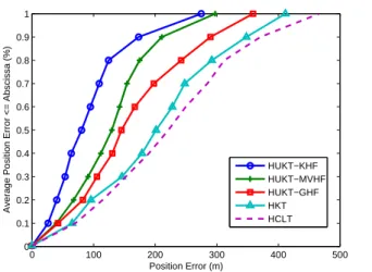
Average Position Error <= Abscissa (%)

HUKT−KHF HUKT−MVHF HUKT−GHF HKT HCLT

Figure 5.3: Performance comparison between the GHF, MVHF, and HUKT-KHF, HKT, and HCLT schemes.

relationship between the MS and the associated BSs. The GHF βg cannot completely react to the operating status of the proposed HUKT scheme which results in the larger position error compared to the other two hybrid factors β_m and β_f. It can be seen that the KHF

β_f can quickly respond to the variations of position error, e.g. larger value β_f is assigned in order to compensate the larger position error at simulation time around 200 sec. Therefore, the proposed HUKT-KHF scheme can provide the smallest average position error of the MS compared to the other two methods.

Fig. 5.3 illustrates the performance comparison of average position errors between the HCLT, HKT, and HUKT scheme associated with the three determination methods for hybrid factors βg, βm, and βf. Note that the two-step LS method is adopted as the location estimator for both the HCLT and HKT schemes as shown in Fig. 1.1. It can be seen that the proposed HUKT algorithms outperform the other two existing schemes, e.g. the HUKT-KHF scheme results in around 160 m less in position error compared to the HKT scheme under 90% of average position error. The estimation accuracy for both the HCLT and the HKT methods rely on the performance of the location estimator. These two-stage schemes induce larger estimation error comparing with the proposed single-stage algorithm, i.e. the HUKT scheme. The nonlinear behavior is also predicted and updated within the HUKT formulation, which results in higher location estimation and tracking accuracy for the MS. Furthermore, similar

0 50 100 150 200 250 300 1 2 3 4 5 6 7 Tme (sec) Number of Bs TOA TDOA

Figure 5.4: The number of available BSs from TOA and TDOA measurements. to the observation in Fig. 5.2, the HUKT-KHF scheme results in the smallest position error in comparison with the HUKT-MVHF and HUKT-GHF methods. The main reason is that the HUKT-KHF algorithm closely follows the Kalman tracking process for adjusting the hybrid factor βf which can effectively reduce the tracking error for the MS.

5.3

Performance Comparison of HUKT Scheme under

Realis-tic Network Scenarios

In this section, the performance comparison between the HUKT, HKT and HCLT schemes are implemented under the realistic network environments with NLOS noises and insufficient number of signal sources. The network scenarios for the simulations is explained as follows. As shown in Fig. 5.7, the BSs deployed in a regular cellular layout are considered to perform TDOA measurements; while the randomly distributed small range sensors conduct TOA measurements for MS’s location tracking. The noise model for TDOA measurements are

n_i,k ∼ N (0, 32400), i.e., 180 meters standard deviation. The RMS delay spread τm is set to 0.1 for TOA measurements and 0.3 for TDOA measurements. Fig. 5.4 illustrates the total number of available BSs for TOA and TDOA measurements respectively during the simulation time of 300 sec. It is noticed that the situation with insufficient signal sources is arranged for

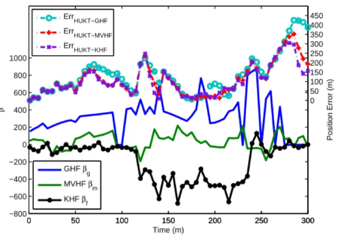
0 50 100 150 200 250 300 −800 −600 −400 −200 0 200 400 600 800 1000 β 0 50 100 150 200 250 300 0 50 100 150 200 250 300 350 400 450 Position Error (m) Time (m) GHF β_g MVHF β m KHF β_f Err HUKT−GHF Err HUKT−MVHF Err HUKT−KHF

Figure 5.5: The position errors associated with the hybrid factors from the proposed HUKT-GHF, HUKT-MVHF, and HUKT-KHF schemes.

the TOA and TDOA BSs, respectively.

Fig. 5.5 shows The position errors along with the corresponding hybrid factors from the proposed HUKT-GHF, HUKT-MVHF, and HUKT-KHF schemes. It can still be observed that the proposed HUKT-KHF scheme can outperform the other two methods under the existence of NLOS noises. Fig. 5.6 illustrates the performance comparison on the average position errors between the HKT, HCLT and the three proposed HUKT schemes. It can be seen that the proposed HUKT-KHF algorithm outperforms all the other schemes, e.g. around 100 m less in position error compared to HKT and HCLT under 67% of average position error. The information of tracking nonlinear behavior provided as feedback to enhance the measurement update within the HUKT formulation, which results in higher location estimation and tracking accuracy for the MS. Finally, the signal insufficiency problem from individual signal path can also be alleviated by adopting the proposed HUKT algorithm.

Figs. 5.7 to 5.9 show the trajectory tracking for the MS’s position, velocity, and accelera-tion. It is noted that the empty circles (as illustrated in Fig. 5.7) represent the locations of the cellular BSs with TOA measurements; while the empty triangles indicates the sensor BSs with TDOA measurements. It can be seen that the proposed HUKT-KHF algorithm can provide better tracking capability comparing with the other two schemes. Both the HCLT and the HKT schemes severely deviate from their true trajectories as the accelerations altered.

Fur-0 100 200 300 400 500 600 0 0.1 0.2 0.3 0.4 0.5 0.6 0.7 0.8 0.9 1 Position Error (m)

Average Position Error <= Abscissa (%)

HUKT−KHF HUKT−MVHF HUKT−GHF HKT HCLT

Figure 5.6: Performance comparison between the GHF, MVHF, and HUKT-KHF, HKT, and HCLT schemes. −1500 −1000 −500 0 500 1000 1500 2000 2500 3000 −2000 0 2000 HUKT−KHF x (m) y (m) −1500 −1000 −500 0 500 1000 1500 2000 2500 3000 −2000 0 2000 HKT y (m) −1500 −1000 −500 0 500 1000 1500 2000 2500 3000 −2000 0 2000 HCLT y (m)

Figure 5.7: Trajectory tracking of the MS using the HCLT, HKT and HUKT-KHF schemes. (solid lines: true trajectories; dotted lines: estimated trajectories; triangles: TDOA BSs; circles: TOA BSs)

0 100 200 300 −40 −20 0 20 40 60 HKT 0 100 200 300 −40 −20 0 20 40 60 HKT Time (sec) 0 100 200 300 −40 −20 0 20 40 60 HUKT−KHF 0 100 200 300 −40 −20 0 20 40 60 HUKT−KHF Time (sec) 0 100 200 300 −50 0 50 100 HCLT vx (m/s) 0 100 200 300 −50 0 50 100 HCLT Time (sec) vy (m/s)

Figure 5.8: Velocity tracking of the MS using the HCLT, HKT and HUKT-KHF schemes. (solid lines: true velocities; dotted lines: estimated velocities)

0 100 200 300 −2 −1 0 1 2 HKT 0 100 200 300 −2 −1 0 1 2 HKT Time (sec) 0 100 200 300 −2 −1 0 1 2 HUKT−KHF 0 100 200 300 −2 −1 0 1 2 HUKT−KHF Time (sec) 0 100 200 300 −50 0 50 HCLT ay (m/s) 0 100 200 300 −50 0 50 HCLT Time (sec) ay (m/s)

Figure 5.9: Acceleration tracking of the MS using the HCLT, HKT and HUKT-KHF schemes. (solid lines: true accelerations; dotted lines: estimated accelerations)

thermore, at the tail of route, insufficiency of signal sources made both the HCLT and HKT unable to maintain accurate location tracking for the MS. The proposed HUKT-KHF algo-rithm can still provide consistent performance (including position, velocity, and acceleration) under the variations of MS’s mobility.

5.4

Performance Comparison of UKT-TOA and UKT-TDOA

Schemes

In this section, the performance of UKT scheme for pure TOA and TDOA measurement inputs are evaluated. The BSs are designed to be located in regular cellular layout for both situation. The noise model for both signals are Gaussian measurement noise with 60 meters standard deviation, i.e. n_i,k ∼ N (0, 3600) and exponential NLOS noise as (5.1) with the RMS

delay spread τ_m = 0.3.

It can be seen in Fig. 5.10 and 5.11 that the simplified special cases of TOA-based and TDOA-based UKT outperform the KT and CLT scheme, which is also consistent to the hybrid operation version. Although the resistance ability to insufficient signal sources is not available due to only sole signal path exists, to additionally track the variation of the nonlinear variable provides better stability and accuracy. The single-stage architecture that directly extract observation result from raw measurement inputs mitigates the common error propagation phenomenon in multiple-stage systems. This unified structure achieves more precision on location estimation and tracking.

0 100 200 300 400 500 600 0 0.1 0.2 0.3 0.4 0.5 0.6 0.7 0.8 0.9 1 Position Error (m)

Average Position Error <= Abscissa (%) UKT−TOA KT CLT

Figure 5.10: Performance comparison between the location tracking schemes for TOA mea-surements. 0 50 100 150 200 250 300 350 400 0 0.1 0.2 0.3 0.4 0.5 0.6 0.7 0.8 0.9 1 Position Error (m)

Average Position Error <= Abscissa (%)

UKT−TDOA KT CLT

Figure 5.11: Performance comparison between the location tracking schemes for TDOA mea-surements.

Chapter 6

Conclusion

In this paper, a hybrid unified Kalman tracking (HUKT) technique is proposed for location estimation and tracking. Based on heterogeneous signal inputs, the HUKT scheme integrates the location estimation and tracking problems within an unified Kalman filtering formulation. The range and range difference measurements from different signal paths are combined based on different designs of hybrid factors. Simulation results show the effectiveness of the HUKT algorithm. Comparing with other existing wireless location techniques, the proposed HUKT scheme can both provide higher precision for mobile location tracking and adapt to insufficient signal sources environments.

Bibliography

[1] Enhanced 911 - Wireless Services. Federal Communication Commission. [Online]. Available: http://www.fcc.gov/911/enhanced/

[2] S. Feng and C. L. Law, “Assisted GPS and Its Impact on Navigation in Intelligent portation Systems,” in Proc. IEEE 5th International Conference on Intelligent

Trans-portation Systems, 2002, pp. 926–931.

[3] Y. Zhao, “Standardization of Mobile Phone Positioning for 3G Systems,” IEEE Commun.

Mag., vol. 40, pp. 108–116, July 2002.

[4] N. Patwari, J. N. Ash, S. Kyperountas, A. O. Hero III, R. L. Moses, and N. S. Correal, “Locating the Nodes: Cooperative Localization in Wireless Sensor Networks,” IEEE

Signal Processing Mag., vol. 22, pp. 54–69, July 2005.

[5] S. Gezici, Z. Tian, G. B. Giannakis, H. Kobayashi, A. F. Molisch, H. V. Poor, and Z. Sahinoglu, “Localization via Ultra-Wideband Radios: A Look at Positioning Aspects for Future Sensor NSetwork,” IEEE Signal Processing Mag., vol. 22, pp. 70–84, July 2005.

[6] T. He, C. Huang, B. M. Blum, J. A. Stankovic, and T. F. Abdelzaher, “Range-Free Localization Schemes in Large Scale Sensor Networks,” in Proc. International Conference

on Mobile Computing and Networking, September 2003.

[8] N. Bulusu, J. Heidemann, and D. Estrin, “Adaptive Beacon Placement,” in Proc. IEEE

International Conference on Distributed Computing Systems, April 2001.

[9] A. J. Weiss, “On the Accuracy of a Cellular Location System Based on RSS Measure-ments,” IEEE Trans. Veh. Technol., vol. 52, pp. 1508–1518, June 2003.

[10] G. G. Raleigh and T. Boros, “Joint Space-Time Parameter Estimation for Wireless Com-munication Channels,” IEEE Trans. Signal Processing, vol. 46, pp. 1333–1343, May 1998. [11] X. Wang, Z. Wang, and B. O’Dea, “TOA-Based Location Algorithm Reducing the Errors due to Non-Line-of-Sight (NLOS) Propagation,” IEEE Trans. Veh. Technol., vol. 52, pp. 112–116, January 2003.

[12] Y. T. Chan and K. C. Ho, “A Simple and Efficient Estimator for Hyperbolic Location,”

IEEE Trans. Signal Processing, vol. 42, pp. 1905–1915, 1994.

[13] W. H. Foy, “Position-Location Solutions by Taylor-series Estimation,” IEEE Trans.

Aerosp. Electron. Syst., vol. 12, pp. 187–194, March 1976.

[14] D. J. Torrieri, “Statistical Theory of Passive Location Systems,” IEEE Trans. Aerosp.

Electron. Syst., vol. 20, pp. 183–198, March 1984.

[15] C. Simon, “A Linear Time-Based Location Technique, Including the Case of Non-Line-Of-Sight,” in Proc. IST Mobile Communications Summit 2001, Sep 2001.

[16] J. J. Caffery, “A New Approach to the Geometry of TOA Location,” in Proc. IEEE

Vehicular Technology Conference, vol. 4, Sep 2000, pp. 1943–1949.

[17] R. O. Schmidt, “A New Approach to Geometry of Range Difference Location,” IEEE

Trans. Aerosp. Electron. Syst., vol. 8, pp. 821–835, Nov 1972.

[18] B. Friedlander, “A Passive Localization Algorithm and its Accurancy Analysis,” IEEE