基於可疑行為及類神經網路之惡意軟體偵測機制

國

立

交

通

大

學

網路工程研究所

碩

士

論

文

基於可疑行為及類神經網路之惡意軟體偵測機制

Suspicious Behavior-based Malware Detection

Using Artificial Neural Network

研 究 生：蔡薰儀

指導教授：王國禎 教授

基於可疑行為及類神經網路之惡意軟體偵測機制

Suspicious Behavior-based Malware Detection

Using Artificial Neural Network

研 究 生：蔡薰儀 Student：Hsun-Yi Tsai

指導教授：王國禎 Advisor：Kuochen Wang

國 立 交 通 大 學

網 路 工 程 研 究 所

碩 士 論 文

Submitted to Institute of Network Engineering College of Computer Science

National Chiao Tung University in partial Fulfillment of the Requirements

for the Degree of Master

in

Computer Science June 2012

Hsinchu, Taiwan, Republic of China

i

基於可疑行為及類神經網路之

惡意軟體偵測機制

學生：蔡薰儀 指導教授：王國禎 博士

國立交通大學網路工程研究所

摘 要

惡意軟體在近幾年非常地盛行，已嚴重危害到電腦及網際網路的

安全。雖然惡意軟體可被些微的修改來躲過傳統字串比對方法的偵測，

但變形過後的惡意軟體仍然與原本的版本有著相同的行為，而這些行

為同時也是其他惡意軟體經常會做的。為了偵測未知的惡意軟體及已

知惡意軟體之變形，在本論文裡我們提出了一個基於可疑行為及類神

經網路之惡意軟體偵測機制，簡稱 ANN-MD。藉著在三個砂盒系統底

下觀察多個已知惡意軟體樣本，我們蒐集並列出了 13 個惡意軟體常

做之可疑行為。利用這 13 個可疑行為，我們提出一個惡意程度表示

式。藉由這個惡意程度表示式，我們可計算出一個未知軟體的惡意程

度值，並根據這個惡意程度值去判定該軟體是否為惡意的。實驗結果

顯示，在測試階段，使用與訓練階段相同的樣本空間的情況下，我們

提出的 ANN-MD 能以 98.1%的正確率辨識出惡意軟體與正常軟體，而

ANN-MD 的誤判率(漏判率) 0.8% (3.0%) 也比 MBF 的誤判率 5.6%

(17.0%)及 RADUX 的誤判率 14.2% (3.4%)小很多。此外，為了進一步

驗證 ANN-MD 的有效性，我們在測試階段使用與訓練階段不相同的樣

本空間來做測試。實驗結果顯示，即使使用與訓練階段不相同的樣本

空間，ANN-MD 的正確率(誤判率)仍可達到 97.0% (5.0%)；然而，MBF

與 RADUX 的正確率(誤判率)卻下降到 77.5% (44.0%)以及 66.0%

(68.0%)。此證明我們所提的 ANN-MD 是一個有效的惡意軟體偵測機

制。

關鍵詞：類神經網路、基於行為比對、惡意軟體偵測、砂盒。

iii

Suspicious Behavior-based Malware

Detection Using Artificial Neural Network

Student：Hsun-Yi Tsai Advisor：Dr. Kuochen Wang

Department of Computer Science National Chiao Tung University

Abstract

In the recent years, malware has been widely spread and has caused severe threats against cyber security. Although malware may be made some changes to evade the traditional signature-based detection, the malware and its variations still have some similar behaviors, which most of the malware also intent to do. In order to detect unknown malware and variations of known ones, we propose a behavioral artificial neural network-based malware detection (ANN-MD) system. By observing runtime behaviors of some known malware samples using three sandboxes, we listed 13 suspicious behaviors that malware frequently did. Then based on these 13 suspicious behaviors, we constructed a malicious degree (MD) expression. By using the MD expression, we can calculate an unknown sample’s MD value and judge whether the sample is a malware according to its MD value. Experimental results indicate that, under the same sample space in the testing phase as well as the training phase, the proposed ANN-MD can correctly discriminate malware from benign software with the accuracy rate of 98.1%. In addition, the false positive rate (false negative rate) of ANN-MD is 0.8% (3.0%), which is much smaller than the false positive rate (false negative rate) of 5.6% (17.0%) of MBF and the false positive rate (false negative rate) of 14.2% (3.4%) of RADUX. To further verify the feasibility of

the proposed ANN-MD, we conducted another experiment by using a different sample space in the testing phase from the sample space used in the training phase. Experimental results show that ANN-MD still has a high accuracy rate of 97.0%, even though the testing sample space is different from the training sample space. However, MBF and RADUX only have the accuracy rates of 77.5% and 66.0%, respectively. In addition, the false positive rate of ANN-MD is 5.0%, which is much smaller than the false positive rate of 44.0% of MBF and the false positive rate of 68.0% of RADUX. This is due to that MBF and RADUX use fixed weights in the training phase. The experimental results support that ANN-MD is a very promising algorithm for malware detection.

v

Acknowledgements

Many people have helped me with this thesis. I deeply appreciate my thesis advisor, Dr. Kuochen Wang, for his intensive advice and guidance. I would like to thank all the members of the Mobile Computing and Broadband Networking Laboratory (MBL) for their invaluable assistance and suggestions. I also want to thank the postdoctoral research fellow of NCTU, Dr. Chia-Yin Lee and Dr. Hao-Chuan Tsai, and Yung-Chi Chang, the engineer of the Network Benchmarking Lab (NBL), NCTU, for helping me with this thesis. Finally, I thank my family for their endless love and support.

Contents

Abstract (Chinese) ... i

Abstract ... iii

Contents ... vi

List of Figures ... viii

List of Tables ... ix

Chapter 1 Introduction ... 1

Chapter 2 Related Work ... 4

Chapter 3 Background ... 7

3.1 Honey-inspector [14]... 7

3.2 Sandbox ... 8

3.3 Artificial neural network ... 9

Chapter 4 Artificial Neural Network-based Behavioral Malware Detection ... 10

4.1 Suspicious behaviors ... 12

4.2 ANN topology ... 15

4.3 MD expression ... 18

Chapter 5 Evaluation ... 19

5.1 Experimental settings ... 19

5.2 MD threshold selection in the training phase ... 21

5.3 Performance of ANN-MD ... 22

5.3.1 Using the same testing and training sample space ... 22

5.3.2 Using different testing sample space from the training sample space ... 24

5.4 Compared with existing schemes ... 25

5.4.1 Using the same testing and training sample space ... 25

vii

Chapter 6 Conclusions and Future Work ... 28

6.1 Concluding remarks ... 28

6.2 Future work ... 29

List of Figures

Figure 1. Architecture of Honey-Inspector [14]. ... 7

Figure 2. The architecture of the proposed ANN-MD. ... 10

Figure 3. Distribution of malicious and benign samples. ... 11

Figure 4. Topology of our artificial neural network... 15

Figure 5. A neuron in the hidden layer. ... 16

Figure 6. A neuron in the output layer [25]. ... 17

Figure 7. Architecture of our ANN (from Matlab). ... 19

Figure 8. Distribution of the numbers of training samples under different MDs. ... 21

Figure 9. The accuracy rate, FPR, and FNR under different MDs. ... 22

Figure 10. Distribution of the numbers of testing samples under different MDs. ... 23

ix

List of Tables

Table 1. Comparison of different behavior-based malware detection algorithms. ... 6 Table 2. The appearance frequencies of malicious and benign samples. ... 14 Table 3. Numbers of benign and malicious samples. ... 20 Table 4. Experimental results using the proposed ANN-MD under the same sample

space. ... 23 Table 5. The FPR, FNR, and accuracy rate under different initial weights. ... 24 Table 6. Experimental results using the proposed ANN-MD under different sample

space. ... 25 Table 7. Comparison of the proposed ANN-MD with two related schemes by using

the same testing and training sample space). ... 26 Table 8. Comparison of the proposed ANN-MD with two related schemes by using

Chapter 1

Introduction

Malware has become one of the most serious security threats to cyber security in recent years. It results in the damage of financial and human resources. To resolve this kind of security problems, many anti-malware (or anti-virus) solutions have been proposed. Existing solutions can be classified into two major categories: i.e., signature-based and behavior-based. The signature-based solutions, like [1] [2], first extract unique digests of the malware to construct the databases of signatures. Next, they use these signatures to check whether unknown binary codes are malicious or not. Therefore, this kind of solutions has a low false positive rate (FPR). However, since the signature-based solutions cannot obtain the signatures of zero-day malware and metamorphic ones at the very first time they emerged, the signature-based solutions may fail to detect them and thus result in high false negative rates (FNR).

In order to detect the zero-day malware or metamorphic malware and decrease FNR, some behavior-based solutions have been proposed [3] [4] [5] [6] [7] [8]. Since malware has some common suspicious behaviors [5], we can use these behaviors to judge whether an unknown sample is malicious. Thus, behavior-based solutions are more effective to detect metamorphic or zero-day malware than signature-based solutions. In addition, behavior-based solutions do not need to update the signatures of malware frequently since suspicious behaviors are almost the same. However, due to benign software might have some behaviors which also appear in malware, it may result in high FPR. Therefore, behavior-based solutions must discover some specific behaviors to distinguish malicious samples from benign ones.

2

Based on the above observations, we contribute the following two respects in this thesis. Firstly, we collect suspicious behaviors which can be used to recognize malicious samples from benign ones. Secondly, we propose an artificial neural network-based malware detection system (ANN-MD), which uses an artificial neural network (ANN) [12] [13] to adjust the weight of each suspicious behavior so as to detect malware effectively. In addition, it can also reduce FPR of malware detection.

Besides, we have implemented a tool chain system, Honey Inspector [14], to actively collect, detect, and analyze malware from Internet. However, the analysis component uses the technology of snapshots to identify malware by checking whether system files are modified. If the characteristics captured by two snapshots before and after executing a sample are different, the sample will be identified as malware. But this method is not effective and not precise enough since it does not consider suspicious behaviors of malware. Thus, one purpose of our work is to improve the performance of the analysis component in the Honey Inspector by using ANN-MD.

In summary, the main objective of our work is to collect distinguishable suspicious behaviors to construct a malicious degree (MD) expression, and then use the MD to identify metamorphic or zero-day malware effectively. We first collect some common suspicious host behaviors, like deleting host files, modifying registry keys, creating files, and so on. These behaviors are mainly inspected by sandboxes [9] [10] [11]. Next, we pick up the most frequent behaviors that appear in malware during runtime and eliminate the behaviors that often appear in normal software during runtime. Then, we train and adjust the weight of each suspicious behavior in the MD expression using an ANN. Finally, we judge whether an unknown sample is a malware using its MD value.

The rest of this thesis is organized as follows. In Chapter 2, we review some related work and discuss the differences among our scheme and related work. In

Chapter 3, we give a brief introduction to the Honey Inspector, sandboxes, and ANNs. In Chapter 4, we illustrate the framework of our scheme and describe some implementation issues. In Chapter 5, experimental results are presented to validate the functionality and the performance of the proposed scheme. Finally, some concluding remarks and future work are given in Chapter 6.

4

Chapter 2

Related Work

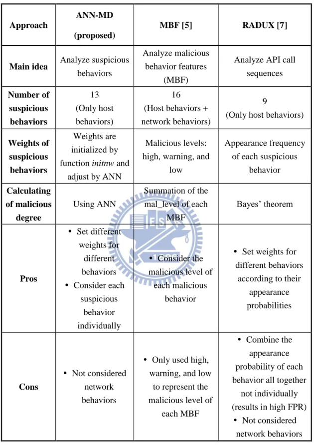
In recent years, many behavior-based malware detection methods have been proposed to overcome the drawbacks of signature-based ones and decrease the FPR of malware detection at the same time. Most of these schemes focus on how to precisely collect the correct and useful behavior information of malware when it is executed [3] [4] [6] [8]. As we illustrate in the previous chapter, our scheme focuses on how to collect common suspicious behaviors and use them to identify malware.

Liu et al. [5] proposed a Malicious Behavior Feature (MBF) based malware detection algorithm to identify malware. An MBF includes three-tuple data: <Feature_id, Mal_level, Bool_expression>. Feature_id is a string identifier which is used to uniquely represent an MBF; Mal_level is an integer weight which divides an MBF into three malicious levels: high, warning, and low; Bool_expression is a Boolean expression which specifically define the behavior of an MBF. A collected MBF is used to calculate an unknown sample’s malicious degree. A sample obtains higher malicious degree if it conforms to more MBFs. MBFs can be used to detect newly out-broken unknown malware. However, since MBFs are divided into three levels, the accuracy rate is relatively low and the FNR is high.

Wang et al. [7] proposed an API-calls-based malware detection prototype, called Reverse Analysis for Detecting Unsafe eXecutable (RADUX). This scheme includes nine suspicious behaviors which are formed by the corresponding API function calls sequences. By using Bayes’ Theorem, they constructed a Bayes expression: ( | ) ∏ ( | ) ( )

samples and ̅ denotes the set of benign samples. ω is the set of those nine malicious behaviors. The appearance probability of a certain behavior ( ) is: P( |C) = the appearance frequency of in set C / the number of malicious samples in C; P( | ̅) = the appearance frequency of in set ̅ / the number of benign samples in ̅. Each sample’s suspicious degree (SD) can be calculated by using this Bayes’ expression. By setting a threshold, the SD value can be used to distinguish malware from benign software. However, the SD expression involves the multiplication of the appearance probability of each suspicious behavior together. The SD expression may results in high FPR, since not all behaviors are inter-dependent.

The main disadvantage of these two schemes [5] [7] is that the malicious level of each suspicious behavior defined is not precise enough. In [5], only three levels are not enough to represent the malicious level of MBF. In [7], the malware detection method may be evaded by using different API call sequences to achieve the same purpose. In order to precisely define the malicious level of each suspicious behavior for detecting malware, we use ANN to train and adjust the weight of each suspicious behavior in our proposed ANN-MD. The details of the proposed ANN-MD are described in Chapter 4. Finally, the Table 1 summarizes the comparison of the proposed ANN-MD with the other two schemes qualitatively.

6

Table 1. Comparison of different behavior-based malware detection algorithms.

Approach

ANN-MD (proposed)

MBF [5] RADUX [7]

Main idea Analyze suspicious

behaviors

Analyze malicious behavior features

(MBF)

Analyze API call sequences Number of suspicious behaviors 13 (Only host behaviors) 16 (Host behaviors + network behaviors) 9

(Only host behaviors)

Weights of suspicious behaviors

Weights are initialized by function initnw and

adjust by ANN

Malicious levels: high, warning, and

low Appearance frequency of each suspicious behavior Calculating of malicious degree Using ANN Summation of the mal_level of each MBF Bayes’ theorem Pros  Set different weights for different behaviors  Consider each suspicious behavior individually  Consider the malicious level of each malicious behavior

 Set weights for different behaviors according to their appearance probabilities Cons  Not considered network behaviors

 Only used high, warning, and low

to represent the malicious level of each MBF  Combine the appearance probability of each behavior all together

not individually (results in high FPR)

 Not considered network behaviors

Chapter 3

Background

3.1 Honey-inspector [14]

Figure 1. Architecture of Honey-Inspector [14].

Honey-Inspector [14] is a tool chain system which can actively collect, detect and analyze malware. Figure 1 shows the architecture of Honey-Inspector. It can be divided into three parts: Collection Subsystem, Detection Subsystem, and Analysis Subsystem. In the Collection Subsystem, there are two ways that Honey-Inspector uses to collect suspicious samples. One is the Web Module that includes a URL blacklist and the other is from the P2P Module that includes P2P-download software. We update the keyword which is used in the P2P Module to search the samples we want via a Keyword Controller in the User Interface. In the Detection Subsystem, Honey-Inspector uses 15 anti-virus software to scan suspicious samples which are

8

collected by the Collection Subsystem. If there are more than 11 of the anti-virus software alarms that the sample is malware, this sample will be sent to the Analysis Subsystem. The Analysis Subsystem will judge whether the suspicious sample is malware by checking the snapshots of system files. Then, it will store the judgment result into the malware library database. Users can obtain samples’ judgment results through Malware Query in the User Interface. As mentioned in Chapter 1, the analysis technology used in the Analysis Subsystem is not effective and not precise enough. Therefore, we aim to improve the malware detection accuracy of the Honey-Inspector by using ANN-MD.

3.2 Sandbox

A sandbox is a virtual machine like testing system which can isolate unknown samples from making changes to the outside system. Since it can perform interactions with malware, malware which is executed under the sandbox can do whatever it wants, e.g. modifying or deleting system files, duplicating several children to conquer the system, connecting to remote servers, or even downloading new update files. But these modifications will not affect the operation of the outside system. And the runtime behaviors of the sample will be recorded and summarized into a report by sandboxes. It is a popular and effective means to gather and analyze the behaviors of malware. There are several malware detection schemes which are based on sandboxes [15] [16] [17] [18]. They used sandboxes to investigate the runtime behaviors of malware. By using their malware detection algorithms, they analyze the reports the sandboxes generated to detect malware. In this thesis, we collect and summarize samples’ behaviors by executing malware in sandboxes. We select three sandboxes, i.e., GFI sandbox [9], Norman sandbox [10], and Anubis sandbox [11] as our analysis platforms to avoid that some sandboxes may be detected by the malware [15] [17].

These sandboxes are popular web-based sandboxes, which are also used by some sandbox-based schemes [15] [16] [17] [18]. We first submit a sample to a sandbox web sites. After executing the sample within a limited duration, the sandbox will summarize the malware’s runtime behaviors into a behavior-based report and send it back. According to the report, we can analyze the sample’s behaviors.

3.3 Artificial neural network

An artificial neural network (ANN) is a kind of machine learning algorithms. It is a calculating system which can mimic the neural network systems of creatures to solve complex problems. An ANN is composed of several interconnected artificial neurons. Each neuron has an I/O characteristic and implements a local computation. The output of a neuron is determined by its I/O characteristic, the interconnecting structure with other neurons, and external inputs [19]. By using simple mathematical techniques and training a plenty of data, the ANN will have the ability of inference and judgment to solve problems [20]. Since the ANN has the ability of fault tolerance and optimization, it can solve extremely complex problems which other algorithms cannot solve. Thus, the ANN is widely used in the computer science fields, e.g. data mining, clustering, classification, prediction, pattern matching, and so on. There are several malware detection schemes which also used the ANN to match the binary code patterns of the malware [21] [22]. In this thesis, use an ANN to classify unknown samples into malware and benign software.

10

Chapter 4

Artificial Neural Network-based

Behavioral Malware Detection

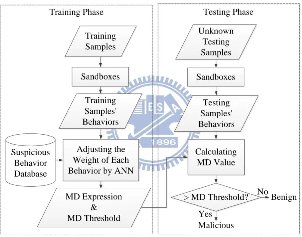
Sandboxes Suspicious Behavior Database Adjusting the Weight of Each Behavior by ANN Sandboxes Calculating MD Value > MD Threshold? Yes No Malicious Benign

Training Phase Testing Phase

Training Samples Training Samples' Behaviors Unknown Testing Samples Testing Samples' Behaviors MD Expression & MD Threshold

Figure 2. The architecture of the proposed ANN-MD.

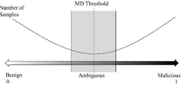
Figure 2 shows the architecture of the proposed ANN-MD. There are two phases in the ANN-MD: training phase and testing phase. The training phase is responsible to train abundant samples, adjust the weights of each behavior using ANN, and then construct an MD expression. First, we collect some common suspicious behaviors identified from three sandboxes [9] [10] [11] and store them in the suspicious

behavior database. Next, we submit the training samples including malicious and benign ones to the sandbox web sites for collecting the runtime behaviors of them. By comparing each sample’s runtime behaviors with the behaviors in the suspicious behavior database, we can train and adjust the weights of each behavior by using ANN. At the end of the training phase, we construct an MD expression. According to the MD values of the training samples, we can set an optimum MD threshold, as shown in Figure 3. The quantities of samples at the two ends of the double-headed arrows line are relatively large. There are a few ambiguous samples at the middle of the line. The optimum MD threshold can discriminate malicious samples from benign samples located at the ambiguous area. The testing phase is responsible to test and judge whether an unknown sample is malicious or not. We first submit the unknown sample to the sandboxes for collecting its runtime behaviors. By using the MD expression which was constructed at the end of training phase, we can calculate the MD value of the unknown sample. If the unknown sample’s MD value is larger than the MD threshold, the unknown sample is identified as malware. Otherwise, it is identified as benign software.

Figure 3. Distribution of malicious and benign samples.

12

4.1 Suspicious behaviors

As mentioned above, we used three sandboxes [9] [10] [11] to collect 13 common suspicious behaviors. We submit samples to these three sandboxes to calculate the appearance frequency of each behavior. We first choose the behaviors in the intersection of the suspicious behaviors identified by these sandboxes and store them to the suspicious behavior database. We eliminate the behaviors which have low appearance frequency or even do not appear (appearance frequency < 15%). Next, we store the behaviors which are not in the intersection but have comparatively high appearance frequency into our database (appearance frequency ≥ 15%), too. The names and descriptions of these 13 suspicious behaviors are listed in the following: 1. Creates Mutex

- Obtains the exclusive access to system recourses [17]. 2. Creates Hidden File

- Creates file without the notification of the user. 3. Starts EXE in System

- Executes EXE without the permission of the user. 4. Checks for Debugger

- Checks whether there is any anti-virus systems under the environment. 5. Starts EXE in Documents

- Documents execute EXE automatically without the permission of the user. 6. Windows/Run Registry Key Set

- Creation, modification, or deletion of Windows registry key. 7. Hooks Keyboard

- Checks keyboard values. 8. Modifies File in System

- Modifies files in the system permanently. 9. Deletes Original Sample

- Deletes the original sample. 10. More than 5 Processes

- Creates more than 5processes. 11. Opens Physical Memory - Accesses physical memory. 12. Delete File in System

- Deletes a file in the system without permission of the user. 13. Auto Start

- Starts automatically when the system reboots.

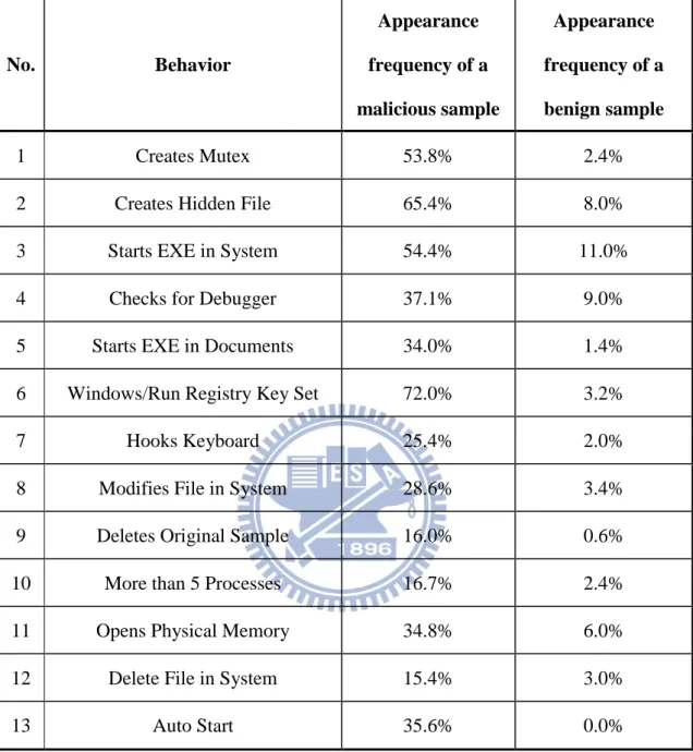
Table 2 shows the appearance frequencies of malicious and benign samples. Note that the suspicious behaviors we chose all have much higher appearance frequencies in malicious samples than that in benign samples.

14

Table 2. The appearance frequencies of malicious and benign samples.

No. Behavior Appearance frequency of a malicious sample Appearance frequency of a benign sample 1 Creates Mutex 53.8% 2.4% 2 Creates Hidden File 65.4% 8.0% 3 Starts EXE in System 54.4% 11.0% 4 Checks for Debugger 37.1% 9.0% 5 Starts EXE in Documents 34.0% 1.4% 6 Windows/Run Registry Key Set 72.0% 3.2% 7 Hooks Keyboard 25.4% 2.0% 8 Modifies File in System 28.6% 3.4% 9 Deletes Original Sample 16.0% 0.6% 10 More than 5 Processes 16.7% 2.4% 11 Opens Physical Memory 34.8% 6.0% 12 Delete File in System 15.4% 3.0% 13 Auto Start 35.6% 0.0%

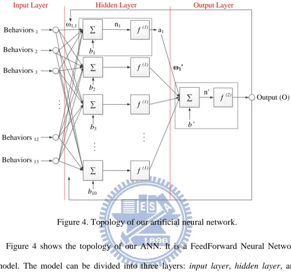
4.2 ANN topology

Input Layer Hidden Layer Output Layer

ƒ (1) ∑ ∑ ∑ ∑ ƒ (1) ƒ (1) ƒ (1) ∑ ƒ (2) a1 ω1' ω1,1 Behaviors 1 Behaviors 2 Behaviors 3 Behaviors 12 Behaviors 13 n1 n'

Figure 4. Topology of our artificial neural network.

Figure 4 shows the topology of our ANN. It is a FeedForward Neural Network model. The model can be divided into three layers: input layer, hidden layer, and output layer. The input layer consists of the suspicious behaviors of an input sample. The hidden layer and output layer contain several neurons which are marked as the dotted line area. If there is more than one hidden layer between the input layer and the output layer, the neural network model will be called as a multi-layer neural network. The major functionality of the hidden layer is to increase the complexity of a neural network. Thus, a multi-layer neural network can resolve more complicated non-linear problems than a single-layer one. The more the number of hidden layers in a neural network is the more complex the neural network will be. However, if there are too many hidden layers in a neural network, it will become an over complex neural network model and may results in over fitting [23]. Thus, it is important to choose the

16

optimum number of the hidden layers and the neurons in them. However, it is regarded as a difficult work to obtain the optimum number of hidden layers and their neurons. At least for now, there is no certain mathematical approach to achieve this goal yet [24]. In the proposed ANN-MD, a two-layer ANN with one hidden layers is founded. In the hidden layer and output layer, we set the number of neurons as 10 and 1, respectively. The operational details of each neuron will be described in the following. . . . b1 a1 n1 Behaviors1 x1 x2 x3 x12 x13 ω1,1 ω2,1 ω3,1 ω12,1 ω13,1 Behaviors2 Behaviors3 Behaviors12 Behaviors13

Figure 5. A neuron in the hidden layer.

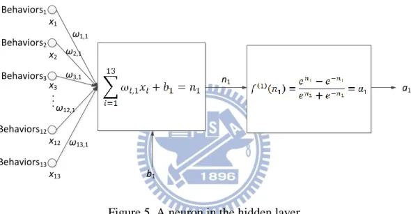
Figure 5 illustrates the operational details of a neuron (the first one) in the hidden layer. The inputs are 13 suspicious behaviors of a sample, i.e. Behaviors1 –

Behaviors13. The input value will be marked as 1 if a sample has the corresponding

suspicious behavior. For example, a sample has No.1, No. 2, No. 6, No. 8 suspicious behaviors, the input data of this sample will be [1, 1, 0, 0, 0, 1, 0, 1, 0, 0, 0, 0, 0]. Multiply these inputs by their corresponding weights in the neuron and do the summation. Then add the neuron’s bias to the summation value. Substitute the result into the transfer function ( )( ) to get the output value of this neuron.

. .

.

a

a

a

a

ω

'

n

’

_O

b

’

ω

'

ω

'

ω

'

Figure 6. A neuron in the output layer [25].

Figure 6 illustrates the details of a neuron in the output layer. The input values of this neuron are a1 – a10, which are the output values of the ten neurons in the hidden

layer. Multiply them by the corresponding weights of each neuron and do the summation. Then add the neuron’s bias to the summation value. Substitute the result into transfer function ( )( ) to get the final output value. We chose the tangent-sigmoid function:

as the transfer functions of our ANN, i.e. ( )( )

18

4.3 MD expression

According to the neural network model mentioned above, we can construct an MD expression. Define set | be a sample’s suspicious behaviors. represents the ith suspicious behavior. Define set { |

| as the weights of suspicious behaviors and the weights of neurons. represents the ith suspicious behavior’s weight in the jth neuron and represents the weight of the kth neuron. Define set | as the bias value of each neuron, where represents the bias value of jth neuron in the hidden layer and represents the bias value of the neuron in the output layer. The MD expression can be represented as follows:

( )_(∑ ( )_(∑ ) )

Both the weight for each behavior and neuron are adjusted through the delta

learning process. Define the mean square error: ( ) , where denotes the target value we gave previously. If a sample is malicious, the target value will be set to 1. On the contrary, will be set to 0. denotes the final output value of the ANN. η , where η represents a learning factor and represents a set of input values. The value ofη is between 0 and 1. The larger the η is the larger the is; however, under these circumstances, the ANN will be more unstable. As a tradeoff, in our scheme, we setη to 0.5. The new weights can be calculated according to the following formula: . The more close to zero the mean square error is, the more convergent and more stable the ANN is.

Chapter 5

Evaluation

5.1 Experimental settings

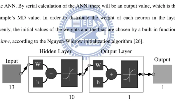
We utilized Matlab 7.11.0 to implement the ANN of our scheme. The architecture of the ANN from Matlab is shown in Figure 7, which is corresponds to that in Figure 4. We take tangent-sigmoid as the transfer functions in both the hidden layer and the output layer. The 13 possible suspicious behaviors of a sample are the input values of the ANN. By serial calculation of the ANN, there will be an output value, which is the sample’s MD value. In order to distribute the weight of each neuron in the layer evenly, the initial values of the weights and the bias are chosen by a built-in function,

initnw, according to the Nguyen-Widrow initialization algorithm [26].

W b + W b + Input 13

Hidden Layer Output Layer

Output

10 1

1

Figure 7. Architecture of our ANN (from Matlab).

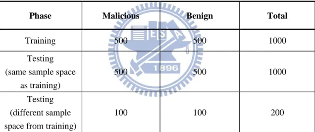
The numbers of malicious and benign samples we used for experiments are shown in Table 3. The size of the sample space is 2200, which is divided into benign samples and malicious samples. We selected 1000 portable execution files which originally exist under the Windows directories after the installation of Windows XP SP2 at the first time as the benign samples. The 1000 malware samples we used were

20

downloaded from Blast’s Security [27] and VX Heaven [28] websites. Among 1000 malicious (benign) samples, 500 (500) samples were used in the training phase and the other 500 (500) samples were used in the testing phase, as shown in Table 3. Besides, to further verifying the feasibility of the proposed ANN-MD, we chose another 200 samples (100 malicious samples and 100 benign samples), which are different from the training sample space. The 100 malicious samples were from the database of National Communications Commission, NCC, of Taiwan (collected by five Internet Service Providers (ISPs) in Taiwan) and the 100 benign samples were downloaded from the CNET.com [29] website.

Table 3. Numbers of benign and malicious samples.

Phase Malicious Benign Total

Training 500 500 1000 Testing

(same sample space as training)

500 500 1000 Testing

(different sample space from training)

100 100 200

We use 9 matrices to evaluate the proposed ANN-MD and the related schemes, as follows:

- True Positive (TP) - False Negative (FN) - False Positive (FP) - True Negative (TN)

- True Positive Rate (TPR) = TP / (TP + FN) - False Negative Rate (FNR) = FN / (TP + FN)

- False Positive Rate (FPR) = FP / (FP + TN) - True Negative Rate (TNR) = TN / (FP + TN) - Accuracy Rate = (TP + TN) / (TP + FN + FP + TN)

5.2 MD threshold selection in the training phase

The distribution of the numbers of training samples is shown as Figure 8. According to this distribution, we can set a possible range of the MD threshold. For benign samples, we choose the largest MD value such that the number of benign samples at this MD value is larger than 10 as the lower bound of the possible range of the MD threshold. For malicious samples, we choose the smallest MD value such that the number of malicious samples at this MD value is larger than 10 as the upper bound of the possible range of the MD threshold. In Figure 8, the possible range of the MD threshold is between 0.19 and 0.87.

Figure 8. Distribution of the numbers of training samples under different MDs. We calculate the accuracy rate, FPR, and FNR under different MDs from 0.19 to 0.87, as shown in Figure 9. First, we narrow down the MD range to MD value =0.5 and MD value=0.59 since the accuracy rates in this range are the highest one, i.e. 98.3

22

%. Then we narrow down the range with the lowest FPR and FNR. Finally, we set the MD threshold as the lowest MD value in this range, i.e. 0.5.

Figure 9. The accuracy rate, FPR, and FNR under different MDs.

5.3 Performance of ANN-MD

5.3.1 Using the same testing and training sample space

In this experiment, we used the same testing sample space as the training sample space to evaluate the performance of the proposed ANN-MD. The experimental results with MD threshold = 0.5 using the proposed ANN-MD are shown in Table 4. It shows that there are only 4 false positive testing samples among the 500 benign testing samples. And the false negative testing samples are 15 among the 500 malicious testing samples. The FPR and the FNR are 0.8% and 3.0%, respectively, which are relatively low compared to two existing schemes [5] [7] which will be shown in Table 7. The accuracy rate of the ANN-MD is 98.1%. Figure 10 illustrates the distribution of the number of testing samples. It shows that ANN-MD can distinguish malicious samples from benign samples with high accuracy.

Table 4. Experimental results using the proposed ANN-MD under the same sample space.

TP TN FP FN FPR FNR Accuracy rate

485 496 4 15 0.8% 3.0% 98.1%

Figure 10. Distribution of the numbers of testing samples under different MDs. We conducted an experiment to evaluate the effects of different initial weights to the proposed ANN-MD. The results are shown in Table 5. It shows that FPR, FNR and accuracy rate for the initial weights chosen by function initnw are the best. And the FPR, FNR and accuracy rate for the initial weights of the hidden layer chosen by the appearance frequency of each behavior are second worse. The worst one is the one without using ANN, where the appearance frequency of each behavior is used to set its corresponding weight. Since this case does not use ANN to train and adjust the weights of each behavior, its accuracy rate is only 93.7%.

24

Table 5. The FPR, FNR, and accuracy rate under different initial weights.

Weights FPR FNR Accuracy rate Adjustment of weights Weights in hidden layer Weights in output layer With ANN Chosen by initnw Chosen by initnw 0.8% 3.0% 98.1% Chosen by appearance frequency Chosen by initnw 1.2% 2.8% 98.0% Without ANN Chosen by appearance frequency 7.8% 4.8% 93.7%

5.3.2 Using different testing sample space from the training

sample space

In order to verify the feasibility of the proposed ANN-MD, we conducted another experiment by using a sample space in the testing phase which is different from the sample space in the training phase.

The experimental results with MD threshold = 0.5 using the proposed ANN-MD are shown in Table 6. It shows that there are 5 false positive samples among the 100 benign samples. The FPR is 5.0%. And there is 1 false negative sample among the 100 malicious samples. The FNR is 1.0%. The accuracy rate of the ANN-MD is 97.0%, which means that the proposed ANN-MD still has a high accuracy rate even using different testing sample space from the training sample space. Figure 11 illustrates the distribution of the numbers of samples under different MDs. It shows that ANN-MD can distinguish malicious samples from benign samples with high accuracy.

Table 6. Experimental results using the proposed ANN-MD under different sample space.

TP TN FP FN FPR FNR Accuracy rate

99 95 5 1 5.0% 1.0% 97.0%

Figure 11. Distribution of the numbers of samples under different MDs.

5.4 Compared with existing schemes

5.4.1 Using the same testing and training sample space

Table 7 shows the comparisons among the proposed ANN-MD and two related schemes, MBF [5] and RADUX [7]. We implemented these two schemes and tested them with the same samples used in the experiment in section 5.3.1. In Table 7, the FPR of ANN-MD is 0.8%; however, the FPR of MBF is 5.6% and the FPR of RADUX is 14.2%. In Table 7, the accuracy rate of ANN-MD is 98.1%; however, the accuracy rate of MBF is only 88.7% and the accuracy rate of RADUX is 91.2%. Table 7 indicates that the proposed ANN-MD is better than MBF and RADUX on unknown malware detection.

26

Table 7. Comparison of the proposed ANN-MD with two related schemes by using the same testing and training sample space).

Approach TPR FNR _Accuracy rate FPR TNR ANN-MD (proposed) 97% 3.0% 98.1% 0.8% 99.2% MBF [5] 83.0% 17.0% 88.7% 5.6% 94.4% RADUX [7] 96.6% 3.4% 91.2% 14.2% 85.8%

5.4.2 Using different testing sample space from the training

sample space

Table 8 shows the comparison among the proposed ANN-MD and two related schemes, MBF [5] and RADUX [7] by using different testing sample space from training sample space). The FPR of ANN-MD is 5.0%; however, the FPR of MBF is 44.0% and the FPR of RADUX is 68.0%. The accuracy rate of ANN-MD is 97.0%; however, the accuracy rate of MBF is only 77.5% and the accuracy rate of RADUX is only 66.0%. Table 8 indicates that the proposed ANN-MD is much better than MBF and RADUX even when using different testing sample space from training sample space. This is due to that MBF and RADUX use static weights in the training phase.

Table 8. Comparison of the proposed ANN-MD with two related schemes by using different testing sample space from the training sample space).

Approach TPR FNR _Accuracy rate FPR TNR ANN-MD (proposed) 99.0% 1.0% 97.0% 5.0% 95.0% MBF [5] 99.0% 1.0% 77.5% 44.0% 56.0% RADUX [7] 100.0% 0.0% 66.0% 68.0% 32.0%

28

Chapter 6

Conclusions and Future Work

6.1 Concluding remarks

In this thesis, we have proposed an artificial neural network-based behavioral malware detection (ANN-MD). By observing and analyzing known malware’s behaviors obtained from sandboxes, we construct a malicious degree (MD) expression. We have collected 13 common suspicious behaviors. We utilized ANN to train and adjust the weight of each behavior to obtain an optimum MD expression. With the MD expression, we can calculate unknown software’s MD value and judge whether the software is malicious or not according to its MD value. Experimental results have shown that the proposed ANN-MD has a high accuracy rate of 98.1% (using the same sample spaces as the training sample spaces), which is better than the accuracy rate of 88.7% in MBF [5] and the accuracy rate of 91.2% in RADUX [7]. In addition, the FPR (FNR) of the proposed ANN-MD is 0.8% (3.0%) (using the same sample spaces as the training sample spaces), which is much smaller than FPR (FNR) of 5.6% (17.0%) in MBF and FPR (FNR) of 14.2% (3.4%) in RADUX. In order to further verify the feasibility of the proposed ANN-MD, we conducted another experiment by using a different sample space in the testing phase from the training phase. Experimental results show that ANN-MD still has a high accuracy rate of 97.0%, even though the testing sample space is different from the training sample space. However, MBF and RADUX only have the accuracy rates of 77.5% and 66.0%, respectively. In addition, the false positive rate of ANN-MD is 5.0%, which is much

smaller than the false positive rate of 44.0% of MBF and the false positive rate of 68.0% of RADUX. This is due to that MBF and RADUX use fixed weights in the training phase. The experimental results have supported that the proposed ANN-MD is a promising methodology in detecting unknown malware and the variations of known malware.

6.2 Future work

In the proposed ANN-MD scheme, we only consider the host behaviors of malware. In addition, the malware detection system we have implemented is semi-automatic, which is time-consuming. Our future work will focus on adding some network suspicious behaviors to our scheme and automating the malware detection system to achieve higher accuracy rate, lower FPR, lower FNR, and faster alarm.

30

References

[1] C. Mihai and J. Somesh, “Static analysis of executables to detect malicious patterns,” in Proceedings of the 12th conference on USENIX Security Symposium, Vol. 12, pp. 169 - 186, Dec. 2006.

[2] J. Rabek, R. Khazan, S. Lewandowskia, and R. Cunningham, “Detection of injected, dynamically generated, and obfuscated malicious code,” in Proceedings

of the 2003 ACM workshop on Rapid malcode, pp. 76 - 82, Oct. 2003.

[3] U. Bayer, C. Kruegel, and E. Kirda, “TTAnalyze: a tool for analyzing malware,” in Proceedings of 15th European Institute for Computer Antivirus Research, Apr. 2006.

[4] M. Egele, C. Kruegel, E. Kirda, H. Yin, and D. Song, “Dynamic spyware analysis,” in Proceedings of USENIX Annual Technical Conference, pp. 233 - 246, Jun. 2007.

[5] W. Liu, P. Ren, K. Liu, and H. X. Duan, “Behavior-based malware analysis and detection,” in Proceedings of Complexity and Data Mining (IWCDM), pp. 39 - 42, Sep. 2011.

[6] A. Moser, C. Kruegel, and E. Kirda, “Exploring multiple execution paths for malware analysis,” in Proceedings of 2007 IEEE Symposium on Security and

Privacy, pp. 231 - 245, May 2007.

[7] C. Wang, J. Pang, R. Zhao, W. Fu, and X. Liu, “Malware detection based on suspicious behavior identification,” in Proceedings of Education Technology and

[8] C. Willems, T. Holz, and F. Freiling. “Toward automated dynamic malware analysis using CWSandbox,” IEEE Security and Privacy, Vol. 5, No. 2, pp. 32 - 39, May 2007.

[9] “GFI Sandbox,” [Online]. Available: http://www.gfi.com/malware-analysis-tool. [10] “Norman Sandbox,” [Online]. Available:

http://www.norman.com/security_center/security_tools.

[11] “Anubis Sandbox,” [Online]. Available: http://anubis.iseclab.org/.

[12] A. Browne, “Neural network analysis, architectures, and applications,” Institute

of Physics Pub., 1997.

[13] T. M. Mitchell, “Artificial neural network,” Machine learning, The McGraw-Hill Companies, Inc. , pp. 81-127, 1997.

[14] “A malware tool chain: active collection, detection, and analysis,” NBL, National Chiao Tung University.

[15] U. Bayer, I. Habibi, D. Balzarotti, E. Krida, and C. Kruege, “A view on current malware behaviors,” in Proceedings of the 2nd USENIX Workshop on

Large-Scale Exploits and Emergent Threats : botnets, spyware, worms, and more,

pp. 1 - 11, Apr. 2009.

[16] H. J. Li, C. W. Tien, C. W. Tien, C. H. Lin, H. M. Lee, and A. B. Jeng, "AOS: An optimized sandbox method used in behavior-based malware detection," in

Proceedings of Machine Learning and Cybernetics (ICMLC), Vol. 1, pp. 404-409,

Jul. 2011.

[17] K. Rieck, T. Holz, C. Willems, P. Dussel, and P. Laskov, “Learning and classification of malware behavior,” in Detection of Intrusions and Malware, and

Vulnerability Assessment, Vol. 5137, pp. 108-125, Oct. 2008.

[18] I. Firdausi, C. Lim, A. Erwin, and A. S. Nugroho, "Analysis of machine learning techniques used in behavior-based malware detection," in Proceedings of the

32

Second International Conference on Advances in Computing, Control and Telecommunication Technologies (ACT), , pp. 201-203, Dec. 2010.

[19] “Prof. Lily Li-Hua Li, CYUT, chapter 1 introduction, artificial neural network (ANN),” [Online]. Available: http://www.cyut.edu.tw/~lhli/ANN/C01-Introduction.pdf.

[20] “ 類 神 經 網 路 基 礎 篇 ,” [Online]. Available: http://mogerwu.blogspot.com/2008/09/blog-post.html.

[21] V. Golovko, S. Bezobrazov, V. Melianchuk, and M. Komar, "Evolution of immune detectors in intelligent security system for malware detection," in

Proceedings of Intelligent Data Acquisition and Advanced Computing Systems (IDAACS), 2011 IEEE 6th International Conference, Vol. 2, pp. 722-726, Sep.

2011.

[22] Y. Zhang, J. Pang, F. Yue, and J. Cui, "Fuzzy neural network for malware detect," in Proceedings of Intelligent System Design and Engineering Application

(ISDEA), 2010 International Conference, Vol. 1, pp. 780-783, Oct. 2010.

[23] “Delight Press, chapter 6, neural network,” [Online]. Available: http://www.delightpress.com.tw/bookRead/skud00013_read.pdf.

[24] Y. Zhang, J. Pang, R. Zhao, and Z. Guo,"Artificial neural network for decision of software maliciousness," in Proceedings of Intelligent Computing and Intelligent

Systems (ICIS), Vol. 2, pp. 622 - 625, Oct. 2010.

[25] C. Weng and K. Wang, “Dynamic resource allocation for MMOG in cloud computing environments,” in Proceedings of IEEE International Wireless

Communications and Mobile Computing Conference (IWCMC), Aug. 2012 (to

appear).

[26] “Neural Network Toolbox,” [Online]. Available: http://dali.feld.cvut.cz/ucebna/matlab/toolbox/nnet/initnw.html.

[27] “Blast's Security,” [Online]. Available: http://www.sacour.cn. [28] “VX heaven,” [Online]. Available: http://vx.netlux.org/vl.php. [29] “CNET,” [Online]. Available: http://www.cnet.com.