影響來台旅客決定性因素探討

全文

(1)國立高雄大學應用經濟學系碩士論文. 影響來台旅客決定性因素探討. On the Determinants of Tourist Arrivals to Taiwan. 研究生：梁慧綺撰指導教授：鄭義暉博士. 中華民國一 ○ 四年一月.

(2) 謝誌轉眼間，碩士班的生活來到了尾聲，喜悅中夾雜著對前方未知的疑慮。回首這兩年半，能夠順利完成論文至畢業，首先要感謝我的指導教授鄭義暉老師，無論是在課業或是待人接物上，老師總是一步一步的帶領著我前進，並且在忙碌中抽空與我討論問題。除此之外，也要感謝論文口試委員佘志民老師與王俊傑老師，給予本論文寶貴的建議以及改進方向，使本論文更加完整。感謝碩士班兩年半幫助過我的同學、學長姐還有學弟妹們，感謝比我早一步畢業的同門夥伴芳茹總是能適時為我解惑，還有一直陪伴在我左右的佳芸學妹。另外，還要感謝把我當掉的老師們，讓我有機會可以重新檢視自己的學習態度與方法，調整後再重頭來一次。比起皆大歡喜的 Happy Ending，這樣踏實的 Real Ending 也許是比較合適的，縱使對未來有些徬徨與焦慮，我仍然會帶著這些日子的收穫繼續前進。最後，感謝家人無條件的支持，讓我在幾年前遭到退學後，還能繼續重拾書本完成學業。一路走來要感謝的人實在太多，謝謝每一個帶給我成長與改變的你。. 梁慧綺中華民國一○四年. i. 立春. 謹誌於. 于高雄大學.

(3) 影響來台旅客決定性因素探討指導教授：鄭義暉. 博士. 國立高雄大學應用經濟學系. 學生：梁慧綺國立高雄大學應用經濟學系碩士班. 摘要. 本研究利用 1993 年至 2013 年交通部觀光局 32 個國家的來台旅客資料，以旅遊引力模型來探討影響來台旅客決定性因素。本研究首先透過資料觀察近年來台旅客的特徵變化，再進行實證分析。針對全部來台旅客資料，控制了特定年份及國家效果後，利用 AIC 和 BIC 比較不同模型的迴歸結果，選出較合適的模型，藉以對觀光與商務來台旅客做進一步分析。根據本文的實證結果，人均所得較高以及與台灣貿易往來較密切的國家會為台灣帶來較多旅客，工業產值較高的國家來台旅客人數也較高。此結果同時也顯示，台灣於 2008 年開放中國大陸旅客來台後，對於日本觀光客的排擠效果並不存在。. 關鍵字：旅遊引力模型、來台旅遊、來台觀光、旅遊流量。. ii.

(4) On the Determinants of Tourist Arrivals to Taiwan. Advisor: Dr. I-Hui Cheng Department of Applied Economics National University of Kaohsiung. Student: Hui-Chi Liang Department of Applied Economics National University of Kaohsiung. Abstract The main purpose of this thesis is to analyze the determinants of tourist arrivals to Taiwan by using gravity-type models of tourism. Firstly this thesis analyzes the tourism data collected by Tourism Bureau of Taiwan, and discusses the characteristic of tourism flows to Taiwan. The data set used in this thesis is a pooled data, consisting of 32 countries, covering years 1993 to 2013. The thesis compares the estimation results of different models, and applies information criteria to examine the goodness of fit for the estimation. Based on the result, a country with higher per capita GDP and a closer trade partner with Taiwan would have more tourist arrivals to Taiwan. To do further analysis, the thesis also estimates tourism flows of for pleasure and for business respectively. The result also supports the argument that after year 2008 the substitution between Chinese and Japanese tourists to Taiwan does not exist statistically.. Keywords: Taiwan tourism, tourist arrivals, tourism flows.. iii.

(5) Contents 謝誌 ........................................................................................................................... i 摘要 .......................................................................................................................... ii Abstract.................................................................................................................... iii Contents ................................................................................................................... iv List of Tables ............................................................................................................. v List of Figures .......................................................................................................... vi 1.. Introduction ....................................................................................................... 1. 2.. Statistical Review of Taiwan’s Inbound Tourism ................................................ 7. 3.. 4.. 5.. 2.1. Basic Information ...................................................................................... 7. 2.2. Main Characteristics of Taiwan’s Inbound Tourism in Recent Years ........... 9. 2.3. The Situation of the Main Tourist Source Markets .................................... 10. The Empirical Model and Data .........................................................................15 3.1. The Empirical Model ............................................................................... 15. 3.2. The Data .................................................................................................. 18. The Estimation Results .....................................................................................19 4.1. The Benchmark Gravity Models .............................................................. 19. 4.2. Controlling for Specific Years and Tourist-origin Countries...................... 21. 4.3. The Model Selection and Estimation Results ............................................ 29. 4.4. Estimating on Pleasure Tourism and Business Tourism ............................ 29. 4.5. A Remark on Year-Specific and Country-Specific Effects ........................ 36. Conclusion .......................................................................................................40. Reference .................................................................................................................43. iv.

(6) List of Tables Table 1. The Numbers and Percentages of International Tourist Arrivals by Region ... 7 Table 2. Top 10 International Tourist Arrivals by Countries ..................................... 10 Table 3. The Definition of Variables ........................................................................ 17 Table 4. The List of Selected 32 Countries and Regions ........................................... 18 Table 5. The Estimation Results of the Benchmark Models...................................... 20 Table 6. The Estimation Results of Total Tourism Flows .......................................... 26 Table 7. The Coefficient Estimates of Year Dummies .............................................. 27 Table 8. The Coefficient Estimates of Country Dummies ......................................... 28 Table 9. The Estimation Results of Pleasure and Business Tourism Flows ............... 35 Table 10. The Coefficient Estimates of Year Dummies............................................. 38 Table 11. The Coefficient Estimates of Country Dummies ....................................... 39. v.

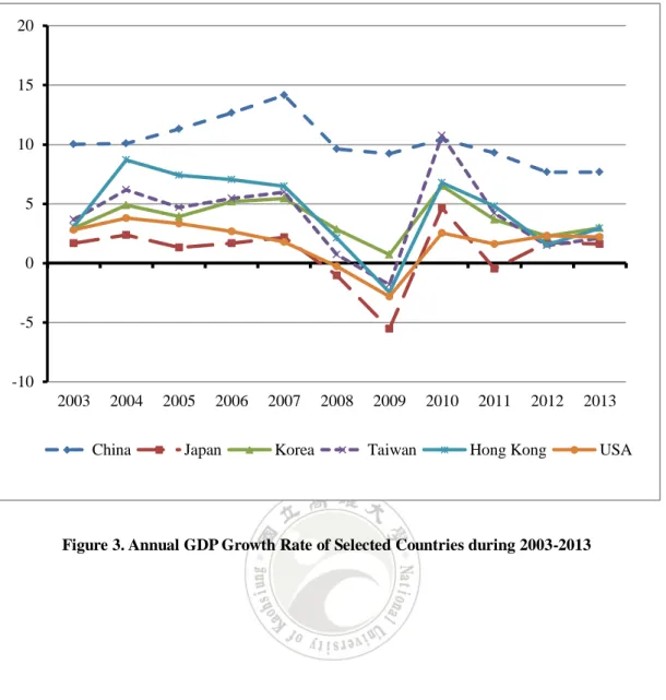
(7) List of Figures Figure 1. Top 3 Countries of Tourist Arrivals to Taiwan during 2008-2013 ………….8 Figure 2. Tourist Arrivals from America and Europe during 2003-2013 ..................... 9 Figure 3. Annual GDP Growth Rate of Selected Countries during 2003-2013 .......... 14. vi.

(8) 1. Introduction All the service activity related to international tourism is essentially a form of international trade, i.e. tourism services export or services import, and better to be considered as a single industry study. According to the World Tourism Organization (henceforth UNWTO in this paper), in 1980 countries’ receipts from international tourism were more than 280 billion dollars, and they already surpassed the one-trillion-dollar mark in a single year after year 2000, accounted for more 10% of the value of international trade annually. Revealing the importance of international tourism, these numbers suggest that better understanding of this industry can promote our empirical understanding in various fields. Firstly, tourism is an important earner of foreign exchange, contributing substantially in financing the imports of foreign capital goods, the current account deficit of the balance of payments, also allows “non-traded goods” to be consumed by inbound tourists. Secondly, tourism spurs investments in new infrastructure, and stimulates services and quality improving competition between firms in tourism industries across countries, and other economic industries by direct and induced effects. Thirdly, tourism directly contributes to generate employment especially for relatively unskilled labors, and indirectly increases tenured employees and the use of temporary employment by firms in the non-traded goods sectors. Finally, but not least important, international tourism provides more opportunity to meet new people, enhances community image and preserves local culture/heritage, and also helps to “promote world peace by providing an incentive for peacekeeping and by building bridges between cultures” (Eilate and Einav, 2004). Some common reasons of tourism program attracting foreign visitors include the economic and social image of the destination country, cultural heritage and cross-border cultural differences, geographical resources, etc. This thesis attempts to 1.

(9) analyze tourist flows from those biggest spenders, namely China, Germany, and the United States, and their impacts of the international tourists on a small open economy like Taiwan.1 By further taking a glimpse on the tourist arrival data of Taiwan for the past few years, in year 2009, China leaped to first place, overtaking both long-time top spender Japan and second largest spender United States. It may due to rising disposable incomes, relaxing restrictions on foreign travel and an appreciating currency in China. 2 Furthermore, the way by which new elected President of Taiwan attempted to have a closer tie with mainland China, responded to the challenge of sluggish growth and also to meet the need of transportation of cross-strait tourists with raising daily entry quota for Chinese tourists, could also reinforce the effects on tourist flows from China to Taiwan.3 Although tourism can bring some economic social benefits, but mass tourism is usually associated with negative effects. For example, in Taiwan, jobs created by tourism are often seasonal and relatively low-paid, while money generated by 1. Based on the UNWTO report, there were 1,035 million international tourist arrivals worldwide,. while international tourism receipts grew to 1,075 billion dollars in year 2012, corresponding to a 4.0% increase in both tourist arrivals and real terms of tourism receipts from year 2011. China, Germany, and the United States are the top three biggest spenders on international tourism for the year 2012, with the market shares 9.5%, 7.8% and 7.7%. When ranking the world’s top international tourist arrivals and international tourism receipts, it is interesting to note that 7 of the top 10 destinations appear on both lists. Countries appearing on both lists include: France, the United States, China, Spain, Italy, Germany, and the United Kingdom (Source: UNWTO Tourism Highlights, 2013 Edition). 2. Chinese travelers have increased their expenditures each year in recent years. In year 2012, they. spent more 102 billion dollars on international tourism and have increased almost eightfold in 12 years, up from 13 billion dollars in year 2000, and bounded to the first place of biggest spenders on international tourism. 3. A new agreement between both governments has reached on the daily quota arrangements of. Mainland Chinese tourists and scheduled direct flights to Taiwan in June 2008.. 2.

(10) Chinese tourism does not always benefit the local community, as most of it leaks out to foreign tourist agency and huge international companies, such as hotel chains. Mass tourism can have a detrimental effect on the quality of life of the local community, e.g. it can push up local property prices and the cost of goods and services, and also cause increased crowding, congestion and pollution through traffic emissions, littering, increased sewage production and noise. Thus, it is interest to examine if Taiwan stands to benefit from being more open to Chinese tourists without substituting the potential tourists from the other major partner countries.4 There are many popular approaches to study the determinants of tourism flows. Vanhove (2005) provides three quantitative methods for forecasting tourism demand, namely univariate time-series methods, regression analysis, and gravity and trip-generation models. Univariate time-series methods such as moving average, exponential smoothing, trend curve analysis, and the Box-Jenkins approach are widely used for forecasting tourism demand (Frechtling, 1996). However, as Vanhove (2005) argues, time-series analysis requires a stable environment for using univariate time-series methods. Regression analysis introduces more than one causal factor, by making turning points and trends being detected. The basic gravity models applied to tourism can pay more attention to the attractiveness between two countries. Trip-generation models are derived from basic gravity models and refine forms of consumer-demand models, which put emphasis on the influence of distance as a constraint of travel. 4. Based on the Key Indicators of Developing Asian and Pacific Countries, in year 2005 China. turned out to be Taiwan’s first-largest trade partner, overtaking Japan and United States. In 2007, Taiwan is the United States’ ninth-largest and Japan’s fourth-largest trading partner, and China’s fifth-largest trading partner. In year 2012, Taiwan is the United States’ eleventh-largest and Japan’s sixth-largest trading partner, and China’s fifth-largest trading partner.. 3.

(11) Crouch et al. (1992) applied conventional economic and marketing theory to measure the effect of marketing efforts on few tourist-origin countries of Australia. Multivariable regression analysis is employed to estimate the elasticities of demand from tourist-origin countries. Their finding suggests that the marketing activities (measured as total expenditure and advertising expenditure) are significant in all countries, and that marketing activities have an important role in affecting tourism inbound is Australia. Borjas (1989) suggests that a model of immigration should include wage earning function for both origin countries and destination countries and moving cost function. Dritsakis and Athanasiadis (2000) build up several explanatory factors to study the variable influencing the tourist demand for Greece. The OLS model is employed in their study to estimate the separate demand functions for each tourist-origin countries. They conclude that Greece continued to attract tourists even under an economic recession, but the tourist host countries would have to face a more demanding, more competitive, and intensely differentiated tourist market in the future. Karemera et al. (2000) examine the influence of political, economic and demographic on the size of migration flows to North America. They argue that population of origin countries, income of destination countries and domestic policy are important factors affecting the migration flows. And less civil freedom has negative effect on migration flows. To capture the possibility of endogeneity and dynamism in tourism, Khadaroo and Seetanah (2008) use a dynamic panel data model of gravity type to evaluate the importance of transport infrastructure, namely the length of pave road, number of airports and ports, and number of hotel rooms, for tourism attractiveness. The data in their research is disaggregated into four subpanels representing different continent of destination and origin. Their result suggests that the level of transport infrastructure 4.

(12) has an importance role in tourist arrivals except for Africa. Saray and Karagöz (2010) use a panel data of 1992-2007 to investigate the effective factors for tourist inflows to Turkey. Using a model of gravity-type, the paper adopts weighted distance as measure of distance between two countries, estimates on per capita GDP and population. Santeramo et al. (2008) examine the tourism demand for non-urbanized rural in Italy. Their study explains the agritourist flows to Italy by applying gravity model and controlling for the effect of rurality and European integration. According to their result, the supply of Italian agritourism should be enhanced due to its advantage in international markets. Su et al. (2010) employ seasonal ARIMA models, focusing on evaluating the impact of Chinese tourists on Taiwan’s international tourism. By examining the monthly tourist arrivals data, they find out that whether the crowding-out effect of Chinese tourists exists in Taiwan’s tourist market and whether the government should keep running the openness policy. According to their finding, the effect may exist for tourists from Japan and United States but not for tourists from Hong Kong. Edwards (1988) introduces two possible of ceilings for tourism demand. First is the annual leave and public holidays out of which the time for tourism is taken. Second is the share of spending on holidays in total expenditure after deal with essential needs. In many countries governors try to handle the ceiling effect by shifting from domestic and international tourism. Kusni et al (2013) investigate the determinants of tourism demand for Malaysia by using a panel data of selected OECD countries during 1995-2009. They argue that tourists from OECD countries are sensitive to the relative price of tourism. Also, they argue that Singapore is a substitute destination of Malaysia, any increase of price in Malaysia would lead to increase the tourist arrivals for Singapore. The number of tourist arrivals to Malaysia has increased during global financial crisis. They suggest that the level of price of 5.

(13) tourism in Malaysia is lower than other neighboring destination, which makes international tourists be able to travel and spend even during recession. Han (2008, in Chinese) uses a panel data of 2000-2005 to analyze how the World Heritage List influences the tourism demand in China. The result suggests that tourism infrastructure, political stability, and numbers of tourist attractions are the key determinants of tourist arrivals to China. Wu (2014, in Chinese) evaluates the effect of international events and disasters on tourism demand for travel to East Asia, using a panel data of 2002-2011. The result shows that relative consumption price is an important factor to affect tourism destination choices. Natural disasters and man-made attacks could also have negative impact on tourism demand. The structure of this thesis is organized as below. Section 2 gives a review of Taiwan’s inbound tourism, which includes the situation of the main tourist source markets surveys literatures of international trade and tourism. Section 3 presents the empirical model of this thesis and the data employed to the estimations. The estimation results and further analysis are presented in Section 4. The conclusion is provided in Section 5.. 6.

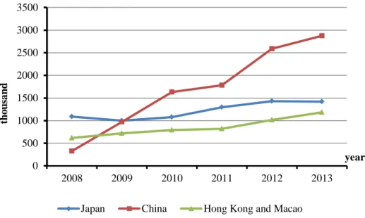
(14) 2. Statistical Review of Taiwan’s Inbound Tourism 2.1 Basic Information Tourism has become an important sector in service GDP for many countries. Over the past two decades, Taiwan’s international tourist arrivals have increased dramatically. Based on the statistics from the Tourism Bureau of Taiwan, the average annual growth rate of total tourist arrivals into Taiwan was 6.09% during 1993-2002, and up to 30.30% during 2003-2013. In 2013, the number of Taiwan’s international tourist arrivals was 8.01 million, an increase more than 100% from 2008. Among the tourist arrivals of Taiwan between 2008 and 2013, tourists from Asia increased from 3.08 million to 7.14 million, America from 461 thousand to 502 thousand, and Europe from 201 thousand to 223 thousand (see Table 1).. . Table 1. The Numbers and Percentages of International Tourist Arrivals by Region Year. 2003. %. 2008. %. 2013. %. Region Advanced.Economies. 1,597,455. 71.06%. 2,844,416. 73.97%. 4,069,177. 50.76%. Emerging.Economies. 312,681. 14.31%. 812,622. 21.13%. 3,818,615. 47.64%. 1,767,640. 78.63%. 3,085,783. 80.25%. 7,138,786. 89.05%. America. 314,721. 14.00%. 461,269. 12.00%. 502,446. 6.27%. Europe. 118,843. 5.29%. 200,914. 5.23%. 223,062. 2.78%. Pacific. 32,330. 1.44%. 68,555. 1.78%. 77,722. 0.97%. Africa. 7,523. 0.33%. 8,499. 0.22%. 8,795. 0.11%. 2,248,117. 100%. 3,845,187. 100%. 8,016,280. 100%. Region Asia. Grand Total. Data Source: Tourism Bureau, M.O.T.C. of Taiwan. In summer 2008, Taiwanese government released new policy which allowed residents from Mainland China to travel into Taiwan. Even under a restricted daily quota of arrivals in the beginning, China surpassed Japan becoming the main tourist 7.

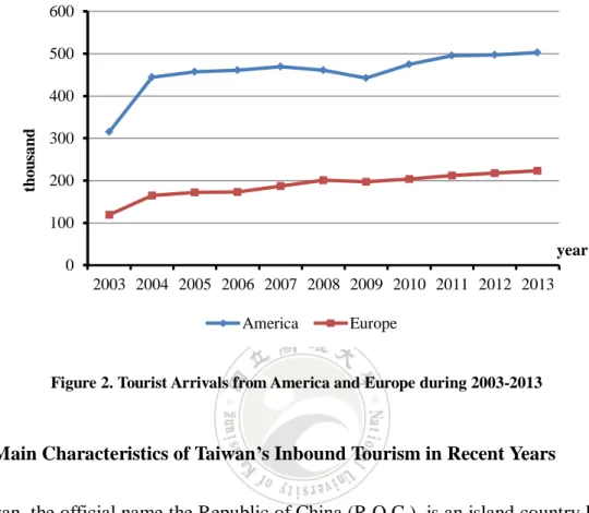
(15) original country for Taiwan in two years. Furthermore, the number of tourist arrivals from China was 329 thousand in 2008 and then dramatically increased to 2.87 million in 2013 (see Figure 1). The number of tourists from Hong Kong and Macao to Taiwan also has a significantly stable growth after 2008, from 618 thousand in 2008, increasing by 91.27% to 1.18 million in 2013. Meanwhile, tourists from Japan to Taiwan also had a steady growth in the past ten years. Although the numbers of tourist arrivals from Japan were 657 thousand, 1.08 million and 1.42 million in 2003, 2008 and 2013, shown as Figure 1, the proportion of Japanese tourists of total tourists to Taiwan was 29.23%, 28.26% and 17.73% in 2003, 2008 and 2013, showing a downward tendency.. 3500 3000 2500. thousand. 2000 1500 1000 500. year. 0 2008 Japan. 2009. 2010 China. 2011. 2012. 2013. Hong Kong and Macao. Figure 1. Top 3 Countries of Tourist Arrivals to Taiwan during 2008-2013. Figure 2 illustrates the trend of tourist arrivals from America and Europe to Taiwan in the last decade. The numbers of tourist arrivals from America were 314 thousand, 461 thousand and 502 thousand in 2003, 2008 and 2013. Meanwhile, the numbers of tourist arrivals from Europe were 118 thousand, 201 thousand and 223 thousand in 2003, 2008 and 2013. Notice that the shares of American and European 8.

(16) tourists were decreasing over years. More detailed data for the shares of regions are listed above in Table 1.. 600 500. thousand. 400 300 200 100 year 0 2003 2004 2005 2006 2007 2008 2009 2010 2011 2012 2013 America. Europe. Figure 2. Tourist Arrivals from America and Europe during 2003-2013. 2.2 Main Characteristics of Taiwan’s Inbound Tourism in Recent Years Taiwan, the official name the Republic of China (R.O.C.), is an island country located in East Asia. The mainland China lies to the west, the Philippines to the south and Japan to the northeast. The total area of Taiwan is 36,193 square kilometers, one tenth of Japan. The grand total population of Taiwan is about 23 million. The Northern Tropic passes through the middle, and makes Taiwan a marine tropical weather. In summer, the whole island of Taiwan has a hot and humid weather, and commonly hit by typhoons each year. The northern part of Taiwan is cold and wet in winter. In contrast, the middle and southern parts have a warm and dry weather in winter. Taiwanese government has established 9 national parks and 13 national scenic areas with various landscape attractions. In 2013, the tourism income of Taiwan was 21.4 billion US dollars, about 5% of grand total GDP. The average expenditure by a 9.

(17) foreign tourist per day was 224.08 US dollars.. 2.3 The Situation of the Main Tourist Source Markets.  Rank. Table 2. Top 10 International Tourist Arrivals by Countries. 2003. 1. Japan. 2. Hong Kong. Arrivals 657,053 323,178. and Macao 3. United States. 2008. Arrivals. Japan Hong Kong. 2013. Arrivals. 1,086,691. China. 2,874,702. 618,667. Japan. 1,421,550. and Macao 272,858. United States. 387,197. Hong Kong. 1,183,341. and Macao 4. Thailand. 98,390. China. 329,204. United States. 414,060. 5. South Korea. 92,893. South Korea. 252,266. Malaysia. 394,326. 6. Philippines. 80,026. Singapore. 205,449. Singapore. 364,733. 7. Singapore. 78,739. Malaysia. 155,783. South Korea. 351,301. 8. Malaysia. 67,014. Indonesia. 110,420. Indonesia. 171,299. 9. Indonesia. 38,078. Philippines. 87,936. Vietnam. 118,467. 10. Canada. 34,369. Thailand. 84,586. Thailand. 104,138. Data Source: Tourism Bureau, M.O.T.C. of Taiwan. 2.3.1 China China ranks the world’s second-largest country by land area next to Russia. The population of China is estimated to be about 1.35 billion in 2013, being the world’s largest country and having 19.24% of world population. The average annual GDP growth rate of China is more than 8% from 1993 to 2013. During the same time, the annual average GDP growth rate of United States is 4.58%. In 2013, China’s GDP was 9.24 trillion US dollars, ranking second economy in the world. But it per capita GDP was about 6,750 US dollars, still far behind most developed countries. 10.

(18) The total exports of China were 2.21 trillion US dollars, with United States, Hong Kong, and Japan being the major trading partners. The total imports of China were 1.95 trillion US dollars, with Japan, South Korea, and Taiwan being the top import partner countries. The exchange rate of China is strictly managed by its central bank, the People’s Bank of China. After 2005, the Chinese government allowed RMB (Reminbi) to float in a relatively restricted range. The total foreign reserve of China was 3.8 trillion US dollars in 2013, ranks the highest in the world.. 2.3.2 Hong Kong and Macao The official name of Hong Kong is Hong Kong Special Administrative Region of the People’s Republic of China. It is close to Pearl River Delta and shares border with Shenzhen City, Guangdong Province, China. Before being an autonomous region of China, Hong Kong was colonized by British government in 1842-1997. The population of Hong Kong is estimated to be about 7.2 million in 2013. Hong Kong economy was shaken by the outbreak of severe acute respiratory syndrome (SARS) in southern China in 2003. After that, GDP of Hong Kong has been a significant growth until now. In 2013, the GDP of Hong Kong was 274 billion, with 38,123 US dollars of per capita GDP. The total exports of Hong Kong were 459 billion US dollars, with China, United States, and Japan being the main export partner countries. The total imports of Hong Kong were 524 billion US dollars, with China, Japan, and Singapore being the top import partner countries. The exchange rate of Hong Kong Dollar is linked to US dollar under a managed float. The total foreign reserve of Hong Kong was 311 billion US dollars in 2013, ranks ninth in the world. Macao, a former Portuguese colony, is one of the two Special Administrative Regions of the People’s Republic of China. It is located in southwest of Hong Kong 11.

(19) and share boarder with Zhuhai City. The sovereignty of Macao was transferred to China from Portugal since 1999. Its population is estimated to be about 615 thousand in 2014. Macao is a densely populated area with a population density of 20,497 people per square mile. The GDP of Macao was 5.3 billion US dollars and 5.9 billion US dollars in 1993 and 1999. It has increased from 6.1 billion to 51.7 billion in 2000-2013, grew by 8 times over this period. During the same period, per capita GDP of Macao has increased from 14,127 US dollars to 91,376 US dollars, ranks fourth in the world. The total foreign reserve of Macao was 16.1 billion.. 2.3.3 Japan Japan is an island nation in East Asia, located in west Pacific Ocean and from the northeast end of Taiwan. It takes 1350 miles flying from Taipei to Tokyo. Japan experienced a population decline since 2007, and its population is about 127.3 million in 2013. In 2013, the GDP of Japan was 4.9 trillion, ranking third in the world with 38,492 US dollars per capita GDP. The total exports of Japan were 715 billion US dollars, with China, United States, and South Korea as the major trading partners, and Taiwan following the fourth place. The total imports of Japan were 832 billion US dollars, with China, United States, and Australia being the major trading partners. After the global financial crisis of 2007-08, the average exchange rate of Japanese Yen appreciated from 117.8 per USD in 2007 to 79.8 per USD in 2011. After Shinzo Abe became prime minister, the Yen weakened to 97.6 in the end of 2013. The total reserve of Japan was 1.26 trillion US dollars in 2013, ranks second in the world.. 2.3.4 South Korea Republic of Korea is in East Asia, located in the southern part of the Korean Peninsula, having a common border with North Korea. There was a diplomatic relation between 12.

(20) South Korea and Taiwan which was terminated in 1992. In 2013, the population of South Korea is about 50.2 million and per capita GDP was 25,976 US dollars in 2013. The total exports of Korea were 560 billion US dollars, with China, United States, and Japan as the major trading partners and Taiwan following the sixth place. The total imports of Korea were 516 billion US dollars, with China, Japan, and United States being the major trading partners. In 2013, the average exchange rate of South Korean Won was 1094.9 to one US dollar, the total foreign reserve of Korea was 345 billion US dollars and ranks eighth in the world.. 2.3.5 The United States The United States is in central of North America, having common border with Canada in North and with Mexico in South. The population of the US is estimated to be 315 million in 2013, being the third largest country in the world and having 4.45% of world population. The annual average GDP growth rate of United States is about 4.58% from 1993 to 2013. In 2013, The United States’ GDP was 16.8 trillion US dollars, being the world largest economy. The per capita GDP of United States was 53,142 US dollars, ranked tenth in the world. The total goods exports of United States were 1.58 trillion US dollars, with Canada, Mexico, and China being the major trading partners. The total goods imports of United States were 2.27 trillion US dollars, with China, Canada, and Mexico being the major trading partners. The trade deficit with China was 317.6 billion US dollars.. 13.

(21) 20. 15. 10. 5. 0. -5. -10 2003. 2004 China. 2005. 2006. Japan. 2007. 2008. Korea. 2009 Taiwan. 2010. 2011. 2012. 2013. Hong Kong. Figure 3. Annual GDP Growth Rate of Selected Countries during 2003-2013. 14. USA.

(22) 3. The Empirical Model and Data 3.1 The Empirical Model The main purpose of this thesis is to study the determinant of the inbound tourism flows to Taiwan. The estimation model of tourism flows can be constructed from the conventional gravity model of bilateral trade. The gravity-type model of trade is based on the gravity theory in physics, the Newton’s law of Universal Gravitation. Normally, the value of bilateral trade flows would increase with the economic sizes of countries and decrease their distance. Thus, the basic gravity equation can be written as 𝑋𝑖𝑗 = 𝛽0 (𝑌𝑖 )𝛽1 (𝑌𝑗 )𝛽2 (𝐷𝑖𝑗 )𝛽3 (𝐴𝑖𝑗 )𝛽4 𝑢𝑖𝑗 ,. (1). where 𝑋𝑖𝑗 is the value of export from country i to country j, 𝑌𝑖 and 𝑌𝑗 are the economic sizes (GDP) of country i and country j respectively, 𝐷𝑖𝑗 the distance between country i to country j, and 𝐴𝑖𝑗 any other factor which would affect the value of trade between two countries. In this study, the estimation model of tourism flows can be specified as 𝑇𝑖𝑗𝑡 = 𝛾0 + 𝛽1 𝐺𝐷𝑃_𝑃𝐶𝑖𝑡 + 𝛽2 𝐷𝐼𝑆𝑇𝑖𝑗 + 𝛽3 𝐼𝑁𝐷𝑖𝑡 + 𝛽4 𝑃𝑂𝑃𝑖𝑡 + 𝛽5 𝑇𝑅𝐴𝐷𝐸𝑖𝑗𝑡 +𝛽6 𝑋𝑅𝑖𝑡 +𝛽7 𝑈𝑅𝐵_𝑃𝑂𝑃𝑖𝑡 + 𝛽8 𝐷𝐸𝐹𝐿𝐴𝑇𝑂𝑅𝑖𝑡 + 𝛽9 𝑌𝐸𝐴𝑅𝑡 + 𝜀𝑖𝑗𝑡 ,. (2) where 𝐺𝐷𝑃_𝑃𝐶𝑖𝑡 is country i’s GDP, 𝐷𝐼𝑆𝑇𝑖𝑗 is the distance between country i and Taiwan (country j), 𝐼𝑁𝐷𝑖𝑡 is the industry value added (percent of GDP) in country i, 𝑃𝑂𝑃𝑖𝑡 is the total population of country i, 𝑇𝑅𝐴𝐷𝐸𝑖𝑗𝑡 is the value of bilateral trade between Taiwan and country i, 𝑋𝑅𝑖𝑡 is the exchange rate to US dollar of country i, 15.

(23) 𝑈𝑅𝐵_𝑃𝑂𝑃𝑖𝑡 is the ratio of urban population to total, and 𝐷𝐸𝐹𝐿𝐴𝑇𝑂𝑅𝑖𝑡 is the GDP deflator of country i. The values of estimator variables except for the dummy variables are measured in logarithmic value except for the year dummy 𝑌𝐸𝐴𝑅. The signs of predicted estimation coefficients are listed below. The explanations of variables are shown in Table 3. β1 > 0: β1 is the coefficient of country i’s per capita GDP. Per capita GDP is usually used as the level of the living standard of a country. Holding all other things constant, people with higher per capita GDP tend to have more leisure and be willing to go abroad. Thus, a country with a higher per capita GDP is expected to have more outbound tourist arrivals to a destination country. β2 < 0: β2 is the coefficient of the distance between two capital cities. Distance between two countries implies the cost of transportation and tourist travel cost. Holding all other things constant, the closer between two countries is, more tourists outbound to a destination country are expected. β3 > 0: β3 is the coefficient of industry value in percent of GDP. Holding all other things constant, a country with higher percent in industry is expected to have more tourist arrivals to Taiwan. β4 > 0: β4 is the coefficient of country i’s population. Holding all other things constant, the more population country i has, the more potential outbound tourists are. Thus, more tourist arrivals to Taiwan are expected. β5 > 0: β5 is the coefficient of trade volume between two countries. Holding all other things constant, the larger trade volume between two countries is expected to have more tourist flow. β6 < 0: β6 is the coefficient of country i’s exchange rate against US dollar. Low exchange rate would lead strong purchasing power on international goods.. 16.

(24) Holding other things constant, the lower exchange rate is expected to have more outbound tourists. β7 > 0: β7 is the coefficient of the urban population ratio. Holding all other things constant, a country with more urban population would have more potential tourist outbound. Thus, more tourist arrivals to Taiwan are expected. β8 ≧ 0 or ≦ 0: β8 is the coefficient of country i’s GDP deflator. It shows the rate of price change in the economy. The estimation can be positive or negative. β9 ≧ 0 or ≦ 0: 𝑌𝐸𝐴𝑅 can be the year dummy or time trend variable. The coefficient estimates can be positive or negative. . Table 3. The Definition of Variables. Variables 𝑇𝑖𝑗𝑡. Definition Total tourist arrivals from country i to j.. Source Tourism Bureau, M.O.T.C. of Taiwan. 𝐺𝐷𝑃_𝑃𝐶𝑖𝑡. GDP per capita is gross domestic product divided by. World Bank. mid-year population. 𝐷𝐼𝑆𝑇𝑖𝑗. The distance between the capital cities of two. Website：How far is it?. countries, expressed in miles. 𝐼𝑁𝐷𝑖𝑡. Industry value added, percent of GDP.. World Bank. 𝑃𝑂𝑃𝑖𝑡. Total population of country i.. World Bank. The total trade between country i and Taiwan.. The Bureau of Foreign. 𝑇𝑅𝐴𝐷𝐸𝑖𝑗𝑡. Trade, M.O.T.C. of Taiwan 𝑋𝑅𝑖𝑡 𝑈𝑅𝐵_𝑃𝑂𝑃𝑖𝑡. The average exchange, local currency per US dollar.. World Bank. The ratio of urban population. The data of population is. World Bank. taken from the World Bank WDI indicators. 𝐷𝐸𝐹𝐿𝐴𝑇𝑂𝑅𝑖𝑡. The GDP deflator is the ratio of nominal (current price) GDP to real GDP.. 𝑌𝐸𝐴𝑅𝑡. Dummy variable of specific year t, or time trend variable. 17. World Bank.

(25) 3.2 The Data To study the determinant of the tourism flows between tourist-origin countries and Taiwan, I construct a data set which consists of 32 countries, covering year 1993 to year 2013, with 578 observations. Table 4 demonstrates the 32 countries included in this study. The independent variables include the per capita GDP of tourist-origin countries, population of origin country, urban population in percent of total, distance between Taiwan and origin countries, total volume of between Taiwan and origin country, exchange rate of origin country, industry value in percent of GDP, GDP deflator of origin country.. . Table 4. The List of Selected 32 Countries and Regions. Asia. America. Europe. Others. Hong Kong, China. Argentina. Austria. Australia. India. Brazil. Belgium. New Zealand. Indonesia. Canada. France. South Africa. Japan. Mexico. Germany. Korea, Republic. United States. Greece. China, People Republic*. Italy. Malaysia. Netherlands. Philippines. Russia*. Singapore. Spain. Thailand. Sweden. Vietnam*. Switzerland United Kingdom. Note *: The data of Hong Kong include Macao, China, from year 2008 to 2013. The data of Russia and Vietnam cover from year 2010 and year 2012 to 2013 respectively.. 18.

(26) 4. The Estimation Results 4.1 The Benchmark Gravity Models The estimation results of the gravity-type benchmark tourism models, the OLS model with time trend and year dummies, are showed in Table 5. The year dummies used to indicate specific years are those when big events or incidents around Taiwan in this study. For instance, Y1997 and Y1998 are used to control for the impact of Asian financial crisis, Y1999 controlling for the effect of the 921 earthquake, and Y2003 controlling for the outbreak of SARS. And, Y2008, Y2009, Y2010, Y2011, Y2012, and Y2013 are controlled for relaxing the strict restrict against residents from Mainland China were allowed to visit Taiwan. In the first column, the OLS model with time trend variable is estimated, controlling for business cycle of the economy. The estimation results of the OLS model with year dummies are shown in second column of Table 5, providing the coefficient estimates of year-specific effects for selected years. Based on the results in Table 5, the tourist arrivals are positively related to per capita GDP and industry value in percent of GDP, and negatively related to the distance between Taiwan and tourist-origin country i. According to the results, holding other constant, a 10% rise in per capita GDP would be associated with a 4.2% increase in tourist arrivals. The more distant between two countries is, the less tourist arrivals would be expected. As shown, holding other constant, a 10% rise in distance would be associated with a 17.8% decrease in tourist arrivals. The ratio of industry value to GDP is employed to examine the effect of the level of industrialization on tourist travel. As shown in Table 5, the coefficient estimate is positive and statistically significant, holding other constant, a 10% rise in percentage of industry would have 7.5% rise in tourist arrivals. 19.

(27) . Table 5. The Estimation Results of the Benchmark Models. GDP per capita. Distance. Industry value. YEAR. OLS with Time Trend. OLS with Year Dummies. lnVTT. lnVTT. 0.416***. 0.417***. (0.046). (0.046). -1.775***. -1.775***. (0.060). (0.060). 0.755***. 0.749***. (0.189). (0.191). 0.00544 (0.008) -0.002. Y1997. (0.231) 0.016. Y1998. (0.231) 0.049. Y1999. (0.231) -0.219. Y2003. (0.231) 0.046. Y2008. (0.224) 0.034. Y2009. (0.228) 0.093. Y2010. (0.228) 0.119. Y2011. (0.228) -0.030. Y2012. (0.232) 0.028. Y2013. (0.240) 7.305. 18.210***. (16.19). (0.951). N. 573. 573. Adj. R2. 0.606. 0.601. AIC. 1782.6. 1799.4. BIC. 1804.3. constant. 1860.3. *. Note: Standard errors in parentheses, p < 0.05,. 20. **. p < 0.01,. ***. p < 0.001..

(28) 4.2 Controlling for Specific Years and Tourist-origin Countries In this subsection, a modified tourism model of gravity-type is used to allow for the heterogeneity of tourist-origin countries and specific years. The estimation results are demonstrated in Tables 6-8. As shown in column (1) of Table 6, the coefficient of per capita GDP is 0.253, being positive and statistically significant, which means that holding other constant, a 10% rise in per capita GDP would be associated with a 2.53% increase in tourist arrivals. The coefficient of distance is -1.958, being negative and statistically significant, indicating that tourist arrivals should decrease 19.58% if the distance between two countries increases by 10%. The coefficient of percentage of industry added-value to total GDP is 0.911, being positive and statistically significant, predicting that holding other tings constant, a 10% rise in the industry value in percent of GDP would be associated with a 9.11% increase in tourist arrivals. The population variable is employed into the model to test if the estimates of the threshold variables are sensitive. In column (2), the coefficient of per capita GDP is 0.755, being positive and statistically significant, which means that holding other constant, a 10% rise in per capita GDP would be associated with a 7.55% increase in tourist arrivals.. The coefficient of distance is -2.224, being negative and statistically. significant, indicating that tourist arrivals should decrease 22.24% if the distance between two countries increases by 10%. The coefficient of percentage of industry added-value to total GDP is 1.172, being positive and statistically significant, predicting that holding other tings constant, a 10% rise in the industry value in percent of GDP would be associated with a 11.72% increase in tourist arrivals. The coefficient of population is 0.507, being positive and statistically significant, which indicates that tourist arrivals should increase 5.07% if the population of country i rises by 10%.. 21.

(29) Next, the variables of bilateral trade flows and the exchange rate in tourist-origin country are also added as an estimator in the model. In column (3), the coefficient of per capita GDP is 0.153, being positive and statistically significant, which means that holding other constant, a 10% rise in per capita GDP would be associated with a 1.53% increase in tourist arrivals. The coefficient of distance is -1.027, being negative and statistically significant, indicating that tourist arrivals should decrease 10.27% if the distance between two countries increases by 10%. The coefficient of percentage of industry value-added to total GDP is 0.540, being positive and statistically significant, predicting that holding other things constant, a 10% rise in the industry value in percent of GDP would be associated with a 5.4% increase in tourist arrivals. The coefficient of population is 0.06, being positive but statistically insignificant, which indicates that tourist arrivals should increase 0.6% if the population of country i rises by 10%. The coefficient of total trade is 0.789, being positive and statistically significant, which means that holding other constant, a 10% rise in total trade should be associated with a 7.89% increase in tourist arrivals. In column (4), the coefficient of per capita GDP is 0.143, being positive and statistically significant, which means that holding other constant, a 10% rise in per capita GDP would be associated with a 1.43% increase in tourist arrivals.. The. coefficient of distance is -1.092, being negative and statistically significant, indicating that tourist arrivals should decrease 10.92% if the distance between two countries increases by 10%. The coefficient of percentage of industry value-added to total GDP is 0.649, being positive and statistically significant, predicting that holding other tings constant, a 10% rise in the industry value in percent of GDP would be associated with a 6.49% increase in tourist arrivals. The coefficient of population is 0.072, being positive but statistically insignificant, which indicates that tourist arrivals should increase 0.72% if the population of country i rises by 10%. The coefficient of total 22.

(30) trade is 0.781, positive and statistically significant, which means that holding other constant, a 10% rise in total trade should be associated with a 7.81% increase in tourist arrivals. The coefficient of exchange rate is -0.028, being negative and statistically insignificant, indicating that tourist arrivals should decrease 0.28% if the exchange rate falls by 10%. To examine whether other social-economic factors drive tourism flows, the variables of urban population ratio and price level are also introduced into the model. In column (5), the coefficient of per capita GDP is 0.069, being positive and statistically significant, which means that holding other constant, a 10% rise in per capita GDP would be associated with a 0.69% increase in tourist arrivals.. The. coefficient of distance is -0.991, being negative and statistically significant, indicating that tourist arrivals should decrease 9.91% if the distance between two countries increases by 10%. The coefficient of percentage of industry added-value to total GDP is 0.568, being positive and statistically significant, predicting that holding other tings constant, a 10% rise in the industry value in percent of GDP would be associated with a 5.68% increase in tourist arrivals. The coefficient of total trade is 0.824, being positive and statistically significant, which means that holding other constant, a 10% rise in bilateral total trade should be associated with a 8.24% increase in tourist arrivals. The coefficient of exchange rate is -0.022, being negative but statistically insignificant, indicating that tourist arrivals should decrease 0.22% if the exchange rate falls by 10%. In column (6), the coefficient of per capita GDP is 0.078, being positive and statistically significant, which means that holding other constant, a 10% rise in per capita GDP would be associated with a 0.78% increase in tourist arrivals. The coefficient of distance is -1.253, being negative and statistically significant, indicating that tourist arrivals should decrease 12.53% if the distance between two countries 23.

(31) increases by 10%. The coefficient of percentage of industry value-added to total GDP is -0.071, being negative and statistically insignificant, predicting that holding other tings constant, a 10% rise in the industry value in percent of GDP would be associated with a 0.71% decrease in tourist arrivals. The coefficient of total trade is 0.844, being positive and statistically significant, which means that holding other constant, a 10% rise in total trade should be associated with a 8.44% increase in tourist arrivals. The coefficient of price level is -0.003, being negative but statistically insignificant, indicating that tourist arrivals should decrease 0.03% if the price level falls by 10%. In column (7), the coefficient of per capita GDP is 0.155, being positive and statistically significant, which means that holding other constant, a 10% rise in per capita GDP would be associated with a 1.55% increase in tourist arrivals.. The. coefficient of distance is -0.96, being negative and statistically significant, indicating that tourist arrivals should decrease 9.6% if the distance between two countries increases by 10%. The coefficient of percentage of industry value-added to total GDP is 0.53, being positive and statistically significant, predicting that holding other tings constant, a 10% rise in the industry value in percent of GDP would be associated with a 5.3% increase in tourist arrivals. The coefficient of total trade is 0.842, being positive and statistically significant, which means that holding other constant, a 10% rise in total trade should be associated with a 8.42% increase in tourist arrivals. The coefficient of exchange rate is -0.027, being negative but statistically insignificant, which means that tourist arrivals should decrease 0.27% if the exchange rate falls by 10% The coefficient of urban population ratio is -0.526, being negative and statistically significant, predicting that tourist arrivals should decrease 5.26% if the urban population ratio falls by 10%. In column (8), the coefficient of per capita GDP is 0.09, being positive and statistically significant, which means that holding other constant, a 10% rise in per 24.

(32) capita GDP would be associated with a 0.9% increase in tourist arrivals.. The. coefficient of distance is -1.255, being negative and statistically significant, indicating that tourist arrivals should decrease 12.55% if the distance between two countries increases by 10%. The coefficient of percentage of industry value-added to total GDP is 0.058, being positive but statistically insignificant, predicting that holding other tings constant, a 10% rise in the industry value in percent of GDP would be associated with a 0.58% increase in tourist arrivals. The coefficient of total trade is 0.846, being positive and statistically significant, which means that holding other constant, a 10% rise in total trade should be associated with an 8.46% increase in tourist arrivals. The coefficient of exchange rate is -0.018, being negative but statistically insignificant, which means that tourist arrivals should decrease 0.18% if the exchange rate falls by 10% The coefficient of urban population ratio is -0.131, being negative but statistically insignificant, predicting that tourist arrivals should decrease 1.31% if the urban population ratio falls by 10%. The coefficient of price level is -0.002, being negative but statistically insignificant, indicating that tourist arrivals should decrease 0.02% if the price level falls by 10%. The estimation results of total tourism flows have been shown above. In next subsection, this thesis turns to make sensitivity analyses and discuss how robust the above results are.. 25.

(33) . GDP per capita. Distance. Industry value. Table 6. The Estimation Results of Total Tourism Flows. (1). (2). (3). (4). (5). (6). (7). (8). lnVTT. lnVTT. lnVTT. lnVTT. lnVTT. lnVTT. lnVTT. lnVTT. 0.253***. 0.755***. 0.153**. 0.143**. 0.069*. 0.078**. 0.155***. 0.091*. (0.035). (0.051). (0.048). (0.048). (0.028). (0.030). (0.035). (0.046). -1.958***. -2.224***. -1.027***. -1.092***. -0.991***. -1.253***. -0.960***. -1.255***. (0.066). (0.062). (0.074). (0.084). (0.065). (0.074). (0.065). (0.085). 0.911***. 1.172***. 0.540***. 0.649***. 0.568***. -0.071. 0.530***. 0.058. (0.173). (0.153). (0.119). (0.136). (0.130). (0.165). (0.128). (0.197). 0.507***. 0.060. 0.072. (0.040). (0.037). (0.038). 0.789***. 0.781***. 0.824***. 0.844***. 0.842***. 0.846***. (0.038). (0.038). (0.031). (0.032). (0.031). (0.032). -0.028. -0.022. -0.027. -0.018. (0.017). (0.017). (0.017). (0.018). -0.526***. -0.131. (0.132). (0.166). population. Bilateral trade. Exchange rate. Urban ratio. Deflator. -0.003. -0.002. (0.028). (0.029). 20.56***. 8.463***. -3.176**. -2.861**. -2.458*. 1.445. -1.533. 1.461. (0.690). (1.133). (1.017). (1.034). (1.015). (1.228). (1.028). (1.241). 573. 573. 573. 573. 573. 508. 573. 508. Adj. R. 0.821. 0.861. 0.922. 0.922. 0.922. 0.907. 0.924. 0.907. AIC. 1349.5. 1205.0. 874.9. 874.2. 875.9. 752.8. 861.4. 755.2. BIC. 1449.6. 1309.4. 983.7. 987.3. 984.7. 858.6. 974.6. 869.4. Constant. N 2. Note: Standard errors in parentheses, * p < 0.05, ** p < 0.01, *** p < 0.001. 26.

(34) . Y1997. Y1998. Y1999. Y2003. Y2008. Y2009. Y2010. Y2011. Y2012. Y2013. Table 7. The Coefficient Estimates of Year Dummies. (1). (2). (3). (4). (5). (6). (7). (8). lnVTT. lnVTT. lnVTT. lnVTT. lnVTT. lnVTT. lnVTT. lnVTT. -0.021. 0.021. -0.024. -0.014. -0.022. -0.032. -0.020. -0.024. (0.155). (0.136). (0.102). (0.102). (0.102). (0.107). (0.101). (0.107). -0.016. 0.069. 0.024. 0.038. 0.024. -0.024. 0.039. -0.006. (0.155). (0.137). (0.102). (0.103). (0.103). (0.113). (0.101). (0.114). 0.023. 0.093. 0.050. 0.042. 0.035. 0.045. 0.045. 0.044. (0.155). (0.136). (0.102). (0.102). (0.102). (0.116). (0.101). (0.117). -0.219. -0.225. -0.222*. -0.223*. -0.222*. -0.221*. -0.215*. -0.218*. (0.155). (0.136). (0.102). (0.102). (0.102). (0.106). (0.101). (0.106). 0.075. -0.178. -0.230*. -0.226*. -0.207*. -0.283**. -0.245*. -0.288**. (0.151). (0.134). (0.101). (0.101). (0.100). (0.104). (0.100). (0.105). 0.044. -0.158. -0.033. -0.025. -0.002. -0.112. -0.026. -0.104. (0.154). (0.136). (0.102). (0.102). (0.102). (0.109). (0.101). (0.109). 0.108. -0.197. -0.244*. -0.235*. -0.212*. -0.317**. -0.246*. -0.313**. (0.153). (0.137). (0.103). (0.103). (0.102). (0.104). (0.101). (0.104). 0.153. -0.208. -0.295**. -0.283**. -0.258*. -0.379***. -0.302**. -0.376***. (0.154). (0.138). (0.104). (0.104). (0.103). (0.104). (0.102). (0.105). 0.203. -0.167. -0.208. -0.195. -0.167. -0.298**. -0.210*. -0.292**. (0.158). (0.142). (0.107). (0.107). (0.106). (0.110). (0.105). (0.110). 0.248. -0.146. -0.171. -0.158. -0.127. -0.284*. -0.162. -0.271*. (0.164). (0.148). (0.111). (0.111). (0.110). (0.117). (0.109). (0.118). Note: Standard errors in parentheses, * p < 0.05, ** p < 0.01, *** p < 0.001.. 27.

(35) . CHN. DEU. JPN. KOR. MYS. PHL. THA. USA. VNM. Table 8. The Coefficient Estimates of Country Dummies. (1). (2). (3). (4). (5). (6). (7). (8). lnVTT. lnVTT. lnVTT. lnVTT. lnVTT. lnVTT. lnVTT. lnVTT. 1.468***. -0.180. -0.013. -0.186. 0.001. -0.083. -0.067. -0.183. (0.361). (0.343). (0.257). (0.278). (0.259). (0.260). (0.257). (0.278). 1.083***. 0.217. -0.127. -0.163. -0.095. -0.072. -0.193. -0.115. (0.176). (0.169). (0.128). (0.130). (0.125). (0.127). (0.126). (0.132). 1.502***. -0.0637. 0.378*. 0.393*. 0.553***. 0.063. 0.546***. 0.105. (0.212). (0.224). (0.169). (0.169). (0.147). (0.308). (0.145). (0.310). -1.107***. -1.835***. -0.784***. -0.768***. -0.652***. -1.059***. -0.533***. -0.990***. (0.230). (0.211). (0.166). (0.166). (0.155). (0.168). (0.155). (0.181). 0.189. 0.454*. 0.116. 0.003. -0.013. -0.090. 0.027. -0.159. (0.207). (0.184). (0.139). (0.155). (0.156). (0.145). (0.154). (0.169). -1.284***. -1.116***. -0.311*. -0.423*. -0.370*. -0.876***. -0.315. -0.882***. (0.229). (0.202). (0.156). (0.171). (0.169). (0.173). (0.167). (0.195). -0.025. 0.014. 0.300*. 0.219. 0.249. 0.089. 0.008. -0.014. (0.212). (0.187). (0.140). (0.149). (0.149). (0.144). (0.158). (0.167). 4.226***. 2.771***. 1.265***. 1.285***. 1.332***. 1.213***. 1.208***. 1.214***. (0.188). (0.202). (0.168). (0.168). (0.166). (0.165). (0.167). (0.168). -0.860. -0.540. -0.436. -0.367. -0.406. -0.754*. -0.551. -0.733. (0.575). (0.507). (0.380). (0.382). (0.382). (0.375). (0.379). (0.378). Note: Standard errors in parentheses, * p < 0.05, ** p < 0.01, *** p < 0.001.. 28.

(36) 4.3 The Model Selection and Estimation Results This study applies information criteria, namely AIC and BIC, to examine the goodness of fit. In the bottom of Table 6, the number of observations, adjusted 𝑅2 , and the information criteria have been provided for each model. The Akaike Information Criterion (AIC), developed by H. Akaike (1973), is a moderate way to measure models for a set of data. For any statistic model, AIC is written as AIC = 2𝑘 − 2 ln 𝐿, where k is the number of parameters in the model, L is the value of maximum likelihood function of the model. According to the criterion, the smaller AIC value is, the better the model is. By giving penalty for the number of parameters, AIC can avoid from a model increasing too many parameters to enhance its goodness of fit. The Bayesian Information Criterion (BIC), also called as the Schwarz criterion, was introduced by E. Schwarz (1978), which is closely related to AIC but giving more penalty weight against using more estimators. BIC can be written as BIC = 𝑘 ln(𝑛) − 2 ln(𝐿), where k is the number of parameters, n is the number of observations or sample size, L is the value of maximum likelihood function of the model. As shown, the BIC penalizes additional parameter more strongly than AIC does.. 4.4 Estimating on Pleasure Tourism and Business Tourism In this subsection, different types of tourism flows are estimated. Based on the information criteria discussed in previous subsection, I choose the models with the smallest BIC value, columns (3), (6)-(8) in Table 6, to estimate on pleasure (lnVTP). 29.

(37) and business (lnVBZ) tourism flows. The estimation results of pleasure tourism and business tourism are shown in columns (1)-(4) and (5)-(8) of Table 9, respectively. As shown in column (1), the coefficient of per capita GDP is 0.108, being positive but statistically insignificant, which means that holding other constant, a 10% rise in per capita GDP would be associated with a 1.08% increase in tourist arrivals for pleasure (TP). The coefficient of distance is -0.771, being negative and statistically significant, indicating that TP should decrease 7.71% if the distance between two countries increases by 10%. The coefficient of percentage of industry value-added to total GDP is 0.463, being positive and statistically significant, predicting that holding other constant, a 10% rise in the industry value in percent of GDP would be associated with a 4.63% increase in tourist arrivals for pleasure. The coefficient of population is -0.221, being negative and statistically significant, which indicates that TP should decrease 2.21% if the population of country i rises by 10%. The coefficient of total trade is 1.163, being positive and statistically significant, which means that holding other constant, a 10% rise in total trade should be associated with an 11.63% increase in tourist arrivals for pleasure. In column (2), the coefficient of per capita GDP is 0.404, being positive and statistically significant, which means that holding other constant, a 10% rise in per capita GDP would be associated with a 4.04% increase in tourist arrivals for pleasure. The coefficient of distance is -1.086, being negative and statistically significant, indicating that TP should decrease 10.86% if the distance between two countries increases by 10%. The coefficient of percentage of industry value-added to total GDP is 0.923, being positive and statistically significant, predicting that holding other constant, a 10% rise in the industry value in percent of GDP would be associated with a 9.23% increase in tourist arrivals for pleasure. The coefficient of total trade is 1.018, being positive and statistically significant, which means that 30.

(38) holding other constant, a 10% rise in total trade should be associated with a 10.18% increase in tourist arrivals for pleasure. The coefficient of price level is 0.05, being positive but statistically insignificant, indicating that TP should increase 0.5% if the price level falls by 10%. In column (3), the coefficient of per capita GDP is 0.16, being positive and statistically significant, which means that holding other constant, a 10% rise in per capita GDP would be associated with a 1.6% increase in tourist arrivals for pleasure. The coefficient of distance is -1.242, being negative and statistically significant, indicating that TP should decrease 12.42% if the distance between two countries increases by 10%. The coefficient of percentage of industry value-added to total GDP is 0.99, being positive and statistically significant, predicting that holding other constant, a 10% rise in the industry value in percent of GDP would be associated with a 9.9% increase in tourist arrivals for pleasure. The coefficient of total trade is 0.999, being positive and statistically significant, which means that holding other constant, a 10% rise in total trade should be associated with a 9.99% increase in tourist arrivals for pleasure. The coefficient of exchange rate is -0.074, being negative and statistically significant, which means that TP should decrease 0.74% if the exchange rate rises by 10%. The coefficient of urban population ratio is 0.773, being positive and statistically significant, predicting that TP should increase 7.73% if the urban population ratio rises by 10%. In column (4), the coefficient of per capita GDP is 0.149, being positive and statistically significant, which means that holding other constant, a 10% rise in per capita GDP would be associated with a 1.49% increase in tourist arrivals for pleasure.. The coefficient of distance is -1.426, being negative and statistically. significant, indicating that TP should decrease 14.26% if the distance between two countries increases by 10%. The coefficient of percentage of industry value-added to 31.

(39) total GDP is 1.179, being positive and statistically significant, predicting that holding other constant, a 10% rise in the industry value in percent of GDP would be associated with a 11.79% increase in tourist arrivals for pleasure. The coefficient of total trade is 0.989, being positive and statistically significant, which means that holding other constant, a 10% rise in total trade should be associated with an 9.89% increase in tourist arrivals for pleasure. The coefficient of exchange rate is -0.092, being negative and statistically significant, which means that TP should decrease 0.92% if the exchange rate rises by 10%. The coefficient of urban population ratio is 0.908, being positive and statistically significant, predicting that TP should increase 9.08% if the urban population ratio falls by 10%. The coefficient of price level is 0.012, being positive but statistically insignificant, indicating that TP should increase 0.12% if the price level rises by 10%. In column (5), the coefficient of per capita GDP is 0.408, being positive and statistically significant, which means that holding other constant, a 10% rise in per capita GDP would be associated with a 4.08% increase in tourist arrivals for business (BZ). The coefficient of distance is -0.883, being negative and statistically significant, indicating that BZ should decrease 8.83% if the distance between two countries increases by 10%. The coefficient of percentage of industry value-added to total GDP is 0.289, being positive and statistically significant, predicting that holding other constant, a 10% rise in the industry value in percent of GDP would be associated with a 2.89% increase in tourist arrivals for business. The coefficient of population is 0.218, being positive and statistically significant, which indicates that BZ should increase 2.89% if the population of country i rises by 10%. The coefficient of total trade is 0.617, being positive and statistically significant, which means that holding other constant, a 10% rise in total trade should be associated with an 6.17% increase in tourist arrivals for business. 32.

(40) In column (6), the coefficient of per capita GDP is 0.093, being positive and statistically significant, which means that holding other constant, a 10% rise in per capita GDP would be associated with a 0.93% increase in tourist arrivals for business. The coefficient of distance is -1.04, being negative and statistically significant, indicating that BZ should decrease 10.4% if the distance between two countries increases by 10%. The coefficient of percentage of industry value-added to total GDP is -1.251, being negative and statistically significant, predicting that holding other constant, a 10% rise in the industry value in percent of GDP would be associated with a 12.51% decrease in tourist arrivals for business. The coefficient of total trade is 0.779, being positive and statistically significant, which means that holding other constant, a 10% rise in total trade should be associated with a 7.79% increase in tourist arrivals for business. The coefficient of price level is -0.038, being negative but statistically insignificant, indicating that BZ should decrease 0.38% if the price level falls by 10%. In column (7), the coefficient of per capita GDP is 0.339, being positive and statistically significant, which means that holding other constant, a 10% rise in per capita GDP would be associated with a 3.39% increase in tourist arrivals for business. The coefficient of distance is -0.641, being negative and statistically significant, indicating that BZ should decrease 6.41% if the distance between two countries increases by 10%. The coefficient of percentage of industry value-added to total GDP is 0.237, being positive and statistically significant, predicting that holding other constant, a 10% rise in the industry value in percent of GDP would be associated with a 2.37% increase in tourist arrivals for business. The coefficient of total trade is 0.791, being positive and statistically significant, which means that holding other constant, a 10% rise in total trade should be associated with a 7.91% increase in tourist arrivals for business. The coefficient of exchange rate is -0.078, 33.

(41) being negative and statistically significant, which means that BZ should decrease 0.78% if the exchange rate rises by 10%. The coefficient of urban population ratio is -1.387, being negative and statistically significant, predicting that BZ should decrease 13.87% if the urban population ratio rises by 10%. In column (8), the coefficient of per capita GDP is 0.225, being positive and statistically significant, which means that holding other constant, a 10% rise in per capita GDP would be associated with a 2.25% increase in tourist arrivals for business.. The coefficient of distance is -0.937, being negative and statistically. significant, indicating that BZ should decrease 9.37% if the distance between two countries increases by 10%. The coefficient of percentage of industry value-added to total GDP is -0.823, being positive and statistically significant, predicting that holding other constant, a 10% rise in the industry value in percent of GDP would be associated with a 8.23% increase in tourist arrivals for business. The coefficient of total trade is 0.795, being positive and statistically significant, which means that holding other constant, a 10% rise in total trade should be associated with an 7.95% increase in tourist arrivals for business. The coefficient of exchange rate is -0.043, being negative and statistically significant, which means that TP should decrease 0.43% if the exchange rate rises by 10%. The coefficient of urban population ratio is -0.817, being negative and statistically significant, predicting that BZ should decrease 8.17% if the urban population ratio rises by 10%. The coefficient of price level is -0.019, being positive but statistically insignificant, indicating that BZ should increase 0.19% if the price level falls by 10%.. 34.

(42) . GDP per capita. Distance. Industry value. population. Table 9. The Estimation Results of Pleasure and Business Tourism Flows. (1). (2). (3). (4). (5). (6). (7). (8). lnVTP. lnVTP. lnVTP. lnVTP. lnVBZ. lnVBZ. lnVBZ. lnVBZ. 0.108. 0.404***. 0.160**. 0.149*. 0.408***. 0.093***. 0.339***. 0.225***. (0.066). (0.044). (0.049). (0.065). (0.043). (0.024). (0.029). (0.036). -0.771***. -1.086***. -1.242***. -1.426***. -0.883***. -1.040***. -0.641***. -0.937***. (0.102). (0.109). (0.090). (0.122). (0.067). (0.060). (0.053). (0.067). 0.463**. 0.923***. 0.990***. 1.179***. 0.289**. -1.251***. 0.237*. -0.823***. (0.165). (0.244). (0.178). (0.282). (0.108). (0.135). (0.106). (0.154). -0.221***. 0.218***. (0.051) Bilateral trade. 1.163. (0.033). ***. 1.018. (0.053). ***. ***. 0.617***. 0.779***. 0.791***. 0.795***. (0.043). (0.046). (0.034). (0.026). (0.025). (0.025). -0.074**. -0.092***. -0.078***. -0.043**. (0.023). (0.025). (0.014). (0.014). 0.773***. 0.908***. -1.387***. -0.817***. (0.183). (0.237). (0.108). (0.129). 0.999. (0.047). Exchange rate. Urban ratio. ***. 0.050. Deflator. (0.041) Constant. -9.815. ***. -12.217. ***. -11.531. ***. 0.989. 0.012. -0.038. -0.019. (0.041). (0.023). (0.022). -10.825. ***. -5.801***. 4.114***. -0.957. 3.722***. (1.409). (1.811). (1.428). (1.775). (0.921). (1.001). (0.847). (0.968). 573. 508. 573. 508. 573. 508. 573. 508. Adj. R. 0.903. 0.859. 0.904. 0.867. 0.909. 0.911. 0.926. 0.918. AIC. 1247.8. 1147. 3. 1238.1. 1118.9. 761.196. 544.692. 639.186. 502.803. BIC. 1356.6. 1351.2. 1233.1. 869.968. 650.454. 752.309. 617.026. N 2. 1253.0 *. Note: Standard errors in parentheses, p < 0.05,. **. p < 0.01,. ***. p < 0.001. 35.

(43) 4.5 A Remark on Year-Specific and Country-Specific Effects The coefficient estimates of year-specific effects for models TP and BZ are shown in Table 10. The dummies Y1997 and Y1998 are used to estimate the impact of Asian financial crisis. According to the results, both coefficient estimates of Y1997 and Y1998 are negative for TP, but positive for BZ. It indicates that although travel to Taiwan for pleasure decreased during Asian financial crisis, but travel to Taiwan for business stays during the period still increased. The dummy variable Y1999 is used to control for the effect of the 921 earthquake. The result shows that the coefficient of Y1999 is negative for TP but positive for BZ, which indicates that travel to Taiwan for pleasure has been shrunk due to the earthquake, but travel to Taiwan for business stays during Year 1999 still increased. All the coefficient estimates of Y1997, Y1998, and Y1999 are statistically insignificant, except for Y1998 in column (7). The dummy variable Y2003 is used to examine for the outbreak of SARS. Based on the estimation results, the coefficients for TP and BZ are all negative and statistically significant, indicating that SARS did defer travel to Taiwan for pleasure as well as for business stays. The dummy variables Y2008-Y2013 are used to control the year effect after year 2008, when Taiwan government relaxed the tourism restriction against residents from Mainland China. For TP, most coefficient estimates are positive except for Y2008, indicating that the year effect is significant after year 2009. For BZ, all coefficient estimates are negative and statistically significant, which means that travel to Taiwan for business stays decreased after 2008. In the following, I turn to discuss tourist-origin country effects of TP and BZ. The results are shown in Table 11. According to the results, by holding other constant, tourist from China, Japan, Malaysia and United States to Taiwan for pleasure are relatively more than the other countries. By contract, tourists travelling 36.

(44) from Germany, South Korea, the Philippines, Thailand and Vietnam to Taiwan for pleasure are significantly less than other countries. In short, the results support the argument that relaxing the restriction on Chinese residents travelling to Taiwan after 2008 does not deter tourists from Japan and United States. That is, the substitution between Chinese and Japanese tourists does not exist statistically. Also, based on the estimation results, business tourists from China, the Philippines, Thailand and Vietnam to Taiwan are relatively less than an average country, while business tourists from Germany and United States are relatively more. This may be due to a closer business tie between Taiwan and its trade partners Germany and United States. However, business tourists from Taiwan’s major competitors, namely China, South Korea and ASEAN countries, are expected to be less than the other countries.. 37.

(45) . Y1997 Y1998 Y1999 Y2003 Y2008 Y2009. (1). (2). (3). (4). (5). (6). (7). (8). lnVTP. lnVTP. lnVTP. lnVTP. lnVBZ. lnVBZ. lnVBZ. lnVBZ. -0.196. -0.164. -0.154. -0.149. 0.097. 0.082. 0.105. 0.108. (0.142). (0.157). (0.140). (0.153). (0.093). (0.087). (0.083). (0.083). -0.177. -0.203. -0.132. -0.162. 0.172. 0.087. 0.206*. 0.141. (0.142). (0.166). (0.141). (0.163). (0.093). (0.092). (0.083). (0.089). -0.182. -0.061. -0.198. -0.128. 0.174. 0.093. 0.151. 0.109. (0.142). (0.172). (0.140). (0.167). (0.093). (0.095). (0.083). (0.091). -0.336*. -0.345*. -0.353*. -0.360*. -0.222*. -0.265**. -0.204*. -0.250**. (0.141). (0.156). (0.140). (0.151). (0.093). (0.086). (0.083). (0.083). -0.023. -0.184. -0.009. -0.072. (0.140). (0.153). (0.138). (0.150). **. *. **. **. 0.441. 0.367. (0.142) Y2010 Y2011 Y2012 Y2013. Table 10. The Coefficient Estimates of Year Dummies. (0.160). 0.433. (0.140). 0.407. (0.156). 0.096. 0.007. 0.108. 0.082. (0.142). (0.153). (0.141). (0.149). 0.069. -0.049. 0.091. 0.055. (0.144). (0.154). (0.142). (0.151). *. 0.288. 0.159. 0.304. (0.148). (0.162). (0.146). 0.348. *. 0.210. (0.153). 0.349. (0.172) *. Note: Standard errors in parentheses, p < 0.05,. **. *. (0.151) p < 0.01,. ***. 0.256 (0.158) 0.293 (0.168). p < 0.001.. 38. -0.481. ***. (0.091) -0.394. ***. (0.093) -0.546. ***. (0.093) -0.605. ***. (0.094) -0.644. ***. (0.097) -0.635. ***. (0.100). -0.454. ***. (0.085) -0.464. ***. (0.089) -0.579. ***. (0.085) -0.631. ***. (0.085) -0.643. ***. (0.089) -0.673. ***. (0.095). -0.500. ***. (0.082) -0.352. ***. (0.083) -0.526. ***. (0.084) -0.596. ***. (0.084) -0.615. ***. (0.087) -0.577. ***. (0.090). -0.513*** (0.082) -0.448*** (0.085) -0.587*** (0.081) -0.654*** (0.082) -0.651*** (0.086) -0.648*** (0.092).

(46) . CHN DEU JPN KOR MYS PHL THA USA VNM. Table 11. The Coefficient Estimates of Country Dummies. (1). (2). (3). (4). (5). (6). (7). (8). lnVTP. lnVTP. lnVTP. lnVTP. lnVBZ. lnVBZ. lnVBZ. lnVBZ. 1.032**. 0.522. 0.213. -0.009. -1.263***. -1.031***. -1.303***. -1.253***. (0.356). (0.383). (0.356). (0.398). (0.233). (0.212). (0.211). (0.217). -0.647***. -0.784***. -0.769***. -0.748***. 0.170. 0.384***. 0.043. 0.203*. (0.177). (0.187). (0.175). (0.189). (0.116). (0.103). (0.104). (0.103). 1.446***. 1.168*. 1.056***. 1.117*. 0.170. -0.180. 0.765***. 0.007. (0.234). (0.454). (0.202). (0.444). (0.153). (0.251). (0.120). (0.242). -0.127. -0.572*. -0.581**. -0.817**. -0.505***. -0.554***. 0.271*. -0.199. (0.230). (0.247). (0.216). (0.259). (0.150). (0.137). (0.128). (0.141). ***. ***. *. 0.165. 0.087. -0.059. -0.214. -0.139. (0.242). (0.126). (0.118). (0.127). (0.132). 0.745. 0.750. (0.192). (0.214). **. **. -0.575. -0.664. 0.464. (0.214) -1.060. ***. -1.396. ***. -0.385. **. -1.198. ***. (0.216). (0.255). (0.232). (0.280). (0.141). (0.141). **. **. *. **. -0.190. -0.329. **. -0.538. -0.620. -0.455. -0.620. -0.396. **. (0.138) -0.970. ***. -0.983*** (0.152) -0.736***. (0.194). (0.212). (0.220). (0.239). (0.127). (0.117). (0.131). (0.130). ***. ***. ***. ***. ***. ***. ***. 0.749***. 0.892. 0.827. 0.991. 1.098. 0.911. 0.834. 0.814. (0.232). (0.243). (0.232). (0.241). (0.152). (0.134). (0.137). (0.131). **. **. *. *. -0.185. -0.690. *. -0.494. -0.720*. (0.540). (0.344). (0.305). (0.312). (0.295). -1.620. -1.574. (0.526). (0.552) *. Note: Standard errors in parentheses, p < 0.05,. **. -1.142. (0.526) p < 0.01,. ***. -1.221. p < 0.001.. 39.

(47) 5. Conclusion Tourism can be measured as an invisible trading item which leads to have more production, employment and improve the richness of a country. In recent years, spending on travel and tourism has become a fast growing part of world total gross, the study on leisure and recreation thus attract much attention. The purpose of this thesis is to test whether tourist arrivals to Taiwan are affected by partner country’s per capita GDP, industry ratio of total GDP, and distance between two countries. Based on the results of the benchmark model, we conclude that tourist arrivals are positively related to per capita GDP and industry ratio of GDP, but negatively related to distance. Furthermore, more variables such as bilateral total trade, population, and exchange rate are added to the estimation. To provide a further analysis, sensitivity analyses and information criteria are employed to investigate how robust the results are. Based on the estimation results, Models (6), (7), and (8) with the smallest values of AIC and BIC are preferred. According to the result shown in Table 6, a country with higher per capita GDP would have more tourist arrivals to Taiwan. All the coefficients of distance are negative, which indicates that origin countries of tourist arrivals are tending to be Taiwan’s neighboring countries. The coefficients of percentage of industry value-added to total GDP are positive except for Model (6), which means that Taiwan attracts more tourists from higher industrialized countries. All the coefficients of bilateral trade value are positive, indicating that a closer trade partner with Taiwan would lead to have more tourist arrivals to Taiwan. To provide a comparison of the estimations, this thesis analyzes the determination of tourist arrivals for different purpose. According to the result in Table 9, TP and BZ have the same coefficient sign for per capita GDP and distance, which is consistent with the benchmark model. The expected signs of coefficients of 40.