A Fair and Efficient SOM-based Feedback Congestion Control in ATM Networks

全文

(1)A Fair and Efficient SOM-based Feedback Congestion Control in ATM Networks Ing-Chau Chang, Sheng-Wen Hsieh Department of Information Management Chaoyang University of Technology, Taichung County, Taiwan, R.O.C. {icchang, s8814610}@cyut.edu.tw ABSTRACT The ATM Forum has chosen the rate-based congestion control for Available Bit Rate (ABR) services. Many rate-based schemes, such as the Forward Explicit Congestion Notification (FECN), the Backward Explicit Congestion Notification (BECN), the Proportional Rate Control Algorithm (PRCA) and the Self-Detective Congestion Control (SDCC), have been proposed. The FECN and BECN schemes use negative feedback rate control. Overall network collapse may occur, if all notification cells of these two schemes in the backward direction experience severe congestion. The PRCA scheme uses positive feedbacks to solve drawbacks of the FECN and BECN schemes, but unfair distributions of the available network bandwidth among ABR VCs may occur. The SDCC scheme use intelligent holding to solve this problem, but it needs to know the bottleneck switch in advance. To resolve problems of the existing rate-based schemes, a new adaptive congestion control scheme, i.e., the SOM-based Feedback Congestion Control (SFCC) scheme, is proposed to achieve high utilization, low cell loss rate and fair bandwidth allocation among ATM ABR VCs in this paper. 1.Introduction The Asynchronous Transfer Mode (ATM) has played a major role in the high-speed networks. Information is transmitted with short fixed-size cells , which consist of 48 bytes of payload and 5 bytes of header. In ATM networks, there are four classes of traffic, i.e., the constant bit rate (CBR), the variable bit rate (VBR), the available bit rate (ABR) and the unspecified bit rate (UBR). For the CBR service, the peak cell rate (PCR) is negotiated at the connection setup and guaranteed by the network for the duration of the connection. The VBR service negotiates the PCR and the sustainable cell rate (SCR) at the connection setup to guarantee throughput of the connection. To improve the utilization of the network bandwidth, the ATM forum [1] has standardized the ABR service, which also requires a number of QoS parameters to be negotiated at the connection setup. The MCR is the minimum cell rate guaranteed by the network. The ICR is the initial cell rate given by the Source End System (SES). The allowed cell rate (ACR), which is in the range of [MCR, PCR], is the real transmission rate of the SES. Finally, the UBR service does not guarantee the QoS and provides the best-effort service. For the CBR and VBR services, the congestion control is administrated by the admission control and bandwidth allocation at the connection setup time.. Maximum network bandwidth allocated to the ABR service is the bandwidth left, which is dynamically changed with time, by the CBR and the VBR. The ABR service offers the possibility of flexible bandwidth renegotiation during the transmission using resource management (RM) cells from the Destination End System (DES) or the intermediate switches. For the congestion control in the ABR service, there are much more problems. The most famous scheme for the ABR congestion control is the Forward Explicit Congestion Notification (FECN)[2-3] by Makrucki in 1992(Figure 1). This method is to control switches on the closed loop from the SES to the DES and to monitor whether the switches will be congested. The switch status is notified by the queue length. For example, when the length of the queue is over 90% of the switch buffer space, the switch is under congestion. Whenever the switch is congested, it starts to mark the EFCI bit in the cell header. At every period of time, the DES will check the received cell to see if there are marked EFCI bits. If so, it will send a RM cell back to the SES. Hence, the SES will lower its ACR rate whenever it receives a RM cell. Otherwise, the SES will raise the ACR by itself. This kind of scheme, which the switch informs the SES of the congestion occurrence and then the SES decreases the ACR rate at the next period of time, is called the negative feedback control. The most serious problem of the negative feedback control is that the RM cell might suffer delay or lost during transmission. When it happens, the SES would misinterpret the network status as non-congested and then increase the ACR. This wrong behavior would cause the network more seriously congested.To resolve problems of the FECN, Newman proposed a new congestion control scheme, i.e., the Backward Explicit Congestion Notification (BECN)[4] in 1993. It also adapts the negative feedback control, but the control loop is shorter than that of the FECN. The control loop is from the SES to the congested switch. In the BECN, every congested switch will inform the SES of the switch by a RM cell. The SES will decrease its ACR to a half whenever it receives the RM cell or otherwise double the ACR at every period of time. SES. Switch. Switch. DES. IF congested Switch set the EFCI=1 IF receives a RM cell then reduce the ACR. IF EFCI=1 then send a RM cell. Figure 1. Forward Explicit Congestion Notification.

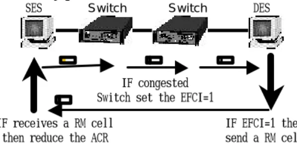
(2) In such a way, the BECN reduces the loss probability of the RM cell by shortening the control loop. Therefore, the BECN can take more instant and correct actions to modify the ACR rate of the ABR VCs than the FECN can do.The remainder of this paper is organized as follows. In section 2, two proposed congestion control schemes are discussed to show their problems. In section 3, details of our SOM-based feedback congestion control scheme are described. It provides the ABR VCs with high utilization, low cell loss rate and fair bandwidth allocation. Simulation results shown in section 4 illustrate the excellent performance of the SFCC scheme. Finally, section 5 concludes this paper.. 2.2 SDCC Akie proposed the Self-Detective Congestion Control (SDCC)[6], which adopts the PRCA loop and feedback controls. For fairness, the SDCC uses the intelligent holding algorithm to calculate the average ABR VC bandwidth needed by the bottleneck switch, and then sends RM cells to the SESs to modify their ACRs to the same value. The most serious problem of SDCC is that it assumes that every ABR VC is aware of its own bottleneck switch. But in the real world, the bottleneck switch may vary with time. Therefore, although the SDCC can solve the fairness problem, it needs a fast algorithm to detect the bottleneck switch on the loop.. 2.Related Works 3. SOM-based Feedback Congestion Control 2.1 PRCA As described above, loss of the RM cell may cause serious problems due to the negative feedback control adopted by both the FECN and the BECN. Therefore, Barnhart proposed the Proportional Rate Control Algorithm (PRCA)[5]. The way to control loop is the same as the FECN but the DES will send a RM cell to the SES when EFCI=0, which means no congestion from the SES to the DES. When the SES receives the RM cell, it will increase the ACR rate; otherwise it will stay still. This kind of method is called the positive feedback control. It will not cause problems as the FECN and the BECN do when the RM cell is lost. The FECN, BECN and PRCA schemes focus on differentiating the control loop and feedback methods to reach high utilization and low cell loss rate. But they cannot provide fair sharing of the available transmission bandwidth among several ABR VCs. Because a switch may deal with many ABR VCs at the same time, it will send the RM cell to the SES of every ABR VC to lower the ACR when congestion occurs. Thus, the SES of all ABR VCs will decrease all their ACRs or increase all their ACRs at the same time to share the bandwidth. It will cause the fairness problem. That is, the VCs with higher ACR use more bandwidth until their connections terminate, but the bandwidth of the VCs with lower ACR keeps low. They cannot have fair bandwidth allocation.. 3.1 Definition of Fairness: In the following, the unfairness behavior of the BECN is illustrated. Assume there have been two VCs transmitted at time 0. One is assumed to be the VBR service type. The VBR traffic is modeled as the Poisson process withλ= 200 cell/ms. Its transmission rate is about 80Mbps. The other VC belongs to the ABR service type and is called as ABR1. Two ABR VCs will arrive at the time 10 and 20 and they are called as ABR2 and ABR3 respectively. The QoS parameters of all ABR VCs are the same: PCR=155Mbps; MCR=0Mbps; the ICR= a cell. The link bandwidth is 155Mbps. The time duration of ABR1 is from 0ms to 200ms (Figure 2), ABR2 from 10ms to 400ms (Figure 3), and ABR3 from 20ms to 600ms (Figure 4). Because ABR1 is the earliest ABR VC, its average transmission rate is around 55Mbps, which is significantly higher than those of ABR2 and ABR3. When the ABR1 connection terminates at 200ms, the ACR rate of ABR2 increases suddenly. Although the ACR rate of ABR3 also increases, it cannot reach the same level as ABR2. Under the BECN, the bandwidth allocation closely depends on the connection setup time.. 0. 100 200 300 400 500 600 Time(ms). Figure 2. Bandwidth use by ABR1 traffic in the BECN. MB(bps). 150 140 130 120 110 100 90 80 70 60 50 40 30 20 10 0. MB(bps). 150 140 130 120 110 100 90 80 70 60 50 40 30 20 10 0. MB(bps). 150 140 130 120 110 100 90 80 70 60 50 40 30 20 10 0. From result of these previous works, none of them could achieve all three criteria, i.e., high utilization, low cells loss rate and fairness. We will propose a new control scheme, which is called the SOM-based Feedback Congestion control (SFCC), and describe details of the SFCC scheme in this section.. 0. 100 200 300 400 500 600 Time(ms). Figure 3. Bandwidth use by ABR2 traffic in the BECN. 0. 100 200 300 400 500 600 Time(ms). Figure 4. Bandwidth use by ABR3 traffic in the BECN.

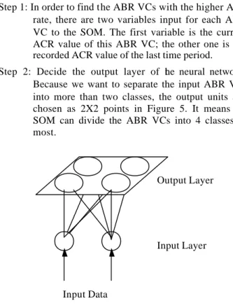
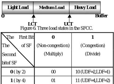
(3) This is because when the congestion occurs, the switch will send RM cells to each ABR VC’s SES. Then all the SESs will decrease their ACR rates to a half. Consequently, the VCs with higher rate remain high but those with lower rate remain low.The basic idea to achieve fairness is rather intuitive. If we want to reduce occurrence of the congestion and achieve the fairness, we may just need to lower those ABR VCs, which consume the major percentage of the available bandwidth. In this way, the ones with lower rates have the chance to get more bandwidth. Whenever the congestion occurs, those ABR connections with the highest ACR rate are found to decrease their rates. In the above example, reducing the ABR1 rate would have more significant influence to resolve the congestion situation. However, there comes a problem. Because each switch may have several ABR VCs at the same time and the situation of every switch may be different and time varying, it is not feasible to define a fixed threshold or a definite function to find the ABR VCs with higher rate. Consequently, the SOM neural network model is used to solve this problem. 3.2 The SOM Neural Network Model: The Self-Organizing Map (SOM)[7] model is an unsupervised learning network model proposed by Kohonen in 1980. The basic concept was come from the cerebrum. The cell in the cerebrum will get together when they have the same functions. The SOM will use these characteristics to cluster the ABR VCs. 3.2.1 The SOM Major Procedure: Step 1: In order to find the ABR VCs with the higher ACR rate, there are two variables input for each ABR VC to the SOM. The first variable is the current ACR value of this ABR VC; the other one is the recorded ACR value of the last time period. Step 2: Decide the output layer of ht e neural network. Because we want to separate the input ABR VCs into more than two classes, the output units are chosen as 2X2 points in Figure 5. It means the SOM can divide the ABR VCs into 4 classes at most.. Output Layer. Input Layer. Input Data Figure 5. Classification operation of the SOM. Step 3: Adjust the output unit Step 3.1: Read the input data of an ABR VC. Compute the distance between this input data and each output unit. Step 3.2: Find the winner unit. The output unit, which has the shortest distance with the input data, is called the winner unit. Step 3.3: Update the winner unit to become more close to the ABR input data. Step 3.4: Repeat 3.1-3.3 for each ABR VC. Step 4: Repeat step 3 for N times to classify the ABR VCs into different classes, where N is a constant. Step 5: From step 4, at most four different ABR VC classes can be generated. For simplicity, four classes can be merged into two parts in the SFCC scheme. The first part is the ABR VC class with the highest ACR rate and the second one is other classes those do not belong to the first part. Two parameters, i.e., the Upper Decrease Factor (UDF) and the Lower Decrease Factor (LDF), are defined for the SES to modify the current ACR values of the two parts respectively. The network manager can define the values of the UDF and LDF at the system initialization time. 3.2.2 Time Complexity of the SOM: From the above steps, it is not difficult to find that the SOM can be completed in linear time. The time complexity is O(Nn) (=O(n)), where n is the number of the ABR VCs and N is the iteration constant at step 4. Consequently, the switch can complete the classification quickly. 3.3 Concept of the SFCC Congestion Control: In order to detect congestion in the BECN and the FECN, queue length of the switch is used for it. Whenever the queue length exceeds the pre-defined threshold of the buffer, it indicates that the switch has lots of cells waiting for transmission. It would begin to discard cells if the buffer overflows. By this way, network congestion can be easily detected. However, this method only uses information to detect current congestion, but it is not able to predict and prevent the forthcoming congestion. In the SFCC, two new parameters are defined as the Upper Congestion Threshold (UCT) and Lower Congestion Threshold (LCT). The buffer space is further divided into three parts, as shown in Figure 6. Each part of the buffer reflects the load state of the switch. They are called as the light load, the medium load and the heavy load. Why this design helps to predict forthcoming congestion? When the buffer is in the medium load, it means the buffer will become congested in the near future. But there is some buffer space available to deal with the incoming cells. The SFCC will decrease the ACR rates as soon as possible to avoid buffer overflow, i.e., to reduce the cell loss rate. Consequently, the SFCC forces the switch to operate in the.

(4) medium load most of the time. In this way, the SFCC can achieve high utilization and low cell loss rate at the same time. We will describe operations in the three load states below.. Light Load. 3.3.2 When the switch is in the medium load. Heavy Load. 0. Buffer LCT UCT Figure 6. Three load states in the SFCC.. 3.3.1 When the switch is in the light load. It means that the system is not congested at this time. In theory, we can inform the SES to increase the ACR by using RM cells. However, it does not mean that the switch would not be congested at the next period of time. If the SES is informed to increase the ACR but the switch become congested at the next period of time, the cell loss would happen. Hence, it is very important to predict the switch load state at the next period of time. The last queue length and the current queue length are used to predict the state of next time. If the current queue length is longer than the last queue length, the queue length of next time will have the trend to grow even longer. In this case, the switch state may change to the medium load or the heavy load. It is not suitable to inform the SES to increase the ACR at this time. Oppositely, if the current queue length is shorter than the last queue length, the switch state at the next period of time may stay in the light load. Compared to traditional schemes, the SFCC would use bandwidth more efficiently and reduce the cell loss rate.. Medium Load. The. First Bit. 0. 1. of SF. (Non-congestion). (Congestion). (Multiply). (Divide). 0 ( by 2). 00. 10 (UDF=2,LDF=1). 1 ( by 4). 01. 11 (UDF=4,LDF=2). The Second bitof SF. Table 1. Meanings of the different SF values 3.4.1 When the switch state is light: IF (last queue length) > (current queue length) then send a RM cell with SF=002 to increase the ACR rate. ELSE do nothing. 3.4.2 When the switch state is medium: use SOM to find the highest ABR VC class. IF (VC) belongs to ( the highest ABR VC class) then. It means that the switch is not congested at this time, but is easy to become congested at the next period of time. In this state, the SFCC will reduce the ACR rate to avoid the switch getting into the heavy load or losing cells. Therefore, we let UDF=2 and LDF=1 in this state. It means that the VC class, which has been classified by the SOM to have the highest ACR rate, will decrease the ACR rate into a half. The other classes do nothing. So the SFCC not only achieves fairness but also reduces the cell loss rate. 3.3.3 When the switch is in the heavy load. It means that the switch is under congestion at this time. The switch buffer will easily overflow, which results in the cell loss. Therefore, the SFCC also uses the SOM and let UDF=4, LDF=2. It can let the switch state leave the heavy load fast to reduce the cell loss rate significantly. 3.4 The SFCC Scheme Operations of the SFCC scheme are listed below. The SFCC uses the first two bits of the “Reserved” field in the RM cell as the new SOM-based Feedback (SF) field. The meanings of the different SF values are listed in table 1. For example, if the SES receives a RM cell with SF=002, it would multiply the current ACR rate by 2 to increase the ACR rate. Oppositely, the ACR rate is divided by 4 if a RM cell with SF=112 is received.. send a RM cell with SF=102 to decrease the ACR rate. ELSE do nothing. 3.4.3 When the switch state is heavy: use SOM to find the highest ABR VC class. IF (VC) belongs to (the highest ABR VC class) then send a RM cell with SF=112 to decrease the ACR rate. ELSE send a RM cell with SF=102 to decrease the ACR rate. 4.Simulation Results In this section, simulation results are shown to demonstrate the performance of the SFFC. It achieves three criteria that we have claimed before. They are: 1.. High link Utilization.. 2.. Low cell loss rate.. 3.. Fairness in bandwidth allocation.. In our simulation, the transmission link bandwidth is 155Mbps and the maximum link utilization is 0.9. It is assumed that a transmission link is shared by 10 VBR and 6 ABR applications where the ABRs are established at different time. The VBRs are assumed to be modeled as Poisson processes ( λ =4 cell/ms, the average bit rate=1.696Mbps). Therefore, the bandwidth needed for the 10 VBRs is 16.96Mbps, which is regarded as the background traffic. The ABR1 arrives at time 0. The ABR2 and the ABR3 arrive at time 100. Finally, the ABR4, the.

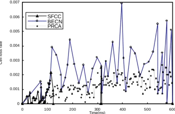
(5) ABR5 and the ABR6 arrive at time 300. All VBR and ABR traffics assume to have the same paths from the SES to the DES. In the following, performances of the BECN, the PRCA and our SFCC are compared. The SDCC is not listed here because it needs to know the bottleneck switch in advance. This is another research issue. 4.1 High link utilization and low cell loss rate: In Figure 7, the BECN threshold is set as 0.9 and the UCT and the LCT of the SFCC are 0.7 and 0.3, respectively. The achieved utilization of the three schemes is high and relatively close. The ABRs of all three schemes can almost consume available bandwidth left after the system initialization time about 180ms. Moreover, the SFCC can push the system to the maximum utilization more than the other two schemes quickly because it can send the RM cell with SF=002 to increase the ACR rate immediately without having to wait as the BECN and the PRCA do. In figure 8, the same parameters (UCT=0.7 and LCT=0.3 for the SFCC; BECN Threshold=0.9) are used to calculate the cell loss rates for the three schemes. The BECN has the highest cell loss rate and then the PRCA. The SFCC has excellent cell loss property. Except the cell loss during the initialization time, the cell loss rate of the SFCC is almost 0. This is the major difference with the other two schemes.. 4.2 Fairness for the bandwidth allocation: First, the ABR bandwidth allocations for the BECN, the PRCA and the SFCC are shown in figure 9-11, figure 12-14 and figure 18-20, respectively. As the given arrival time of ABRs, the ABR1s in the BECN and PRCA schemes consume almost all available bandwidth. Other ABRs nearly cannot share the bandwidth. Oppositely, whenever the new ABRs arrive to the system at time 100 and 300, the SFCC can adjust the bandwidth allocation of all ABRs quickly to the same level. In a word, the SFCC can achieve the Fairness criterion. Second, the fairness achieved by the SOM model and the fixed threshold method for the SFCC is shown in Figure 18-20 and Figure 15-17, respectively. The 128 cells/ms for the ACR rate is chosen as the fixed threshold. Whenever the original SOM is activated in the SFCC scheme, all ABR VCs are classified into two classes with respect to the fixed threshold. One class contains the ABR VCs with their ACR rates higher than the threshold and the other class contains the ABR VCs with lower ACR rates. The rates of the two classes are modified as the original SOM SFCC does. As shown in figure 18-20, the fairness by the fixed threshold method is improved than that of the BECN (figure 9-11). But it is significantly inferior to that of the SOM SFCC (figure 18-20). As described before, it is not feasible to choose a fixed optimal value for the dynamic network environment. Consequently, the SOM model is greatly helpful for the fairness criterion in the SFCC scheme. 0.007. 1. SFCC BECN PRCA. 0.006. 0.9 0.8. 0.005 Cell loss rate. Utilization. 0.7 0.6 0.5. 0.004. 0.003. 0.4 0.002 0.3. BECN SFCC PRCA. 0.2 0.1. 0.001. 0 0. 0 0. 100. 200. 300. 400. 500. Time(ms). 100. 200 300 400 Time(ms). 500. 600. Figure 9. Bandwidth use by ABR1 traffic in BECN. 300 Time(ms). 400. 500. Mbps. 150 140 130 120 110 100 90 80 70 60 50 40 30 20 10 0. Mbps. Mbps. 150 140 130 120 110 100 90 80 70 60 50 40 30 20 10 0. 0. 200. 0. 100. 600. Figure 8. The cell loss rates of the BECN, the PRCA and the SFCC schemes. Figure 7. The Utilization of the BECN, the PRCA and the SFCC schemes 150 140 130 120 110 100 90 80 70 60 50 40 30 20 10 0. 100. 600. 200. 300 400 Time(ms). 500. 600. Figure 10. Bandwidth use by ABR2 and ABR3 traffic in BECN. 0. 100. 200 300 400 Time(ms). 500. 600. Figure 11. Bandwidth use by ABR4, ABR5 and ABR6 traffic in BECN.

(6) 150 140 130 120 110 100 90 80 70 60 50 40 30 20 10 0. 150 140 130 120 110 100 90 80 70 60 50 40 30 20 10 0. 0. 100. 200 300 400 Time(ms). 500. 600. Figure 12. Bandwidth use by ABR1 traffic in PRCA. 0. 100. 200 300 400 Time(ms). 500. 600. Figure 13. Bandwidth use by ABR2 and ABR3 traffic in PRCA. 100. 200 300 400 Time(ms). 500. 600. Figure 15. Bandwidth use by ABR1 traffic in fixed threshold SFCC. 0. 100. 200. 300 400 Time(ms). 500. Figure 16. Bandwidth use by ABR2 and ABR3 traffic in fixed threshold SFCC. 100. 200. 300 400 Time(ms). 500. 600. Figure 18. Bandwidth use by ABR1 traffic in SFCC. 300 400 Time(ms). 500. 600. 0. 100. 200. 300 400 Time(ms). 500. 600. Figure 17. Bandwidth use by ABR4, ABR5 and ABR6 traffic in fixed threshold SFCC. Mbps. 150 140 130 120 110 100 90 80 70 60 50 40 30 20 10 0. Mbps 0. 200. Figure 14. Bandwidth use by ABR4, ABR5 and ABR6 traffic in PRCA. 600. 150 140 130 120 110 100 90 80 70 60 50 40 30 20 10 0. Mbps. 150 140 130 120 110 100 90 80 70 60 50 40 30 20 10 0. 100. 150 140 130 120 110 100 90 80 70 60 50 40 30 20 10 0. Mbps 0. 0. Mbps. 150 140 130 120 110 100 90 80 70 60 50 40 30 20 10 0. Mbps. 150 140 130 120 110 100 90 80 70 60 50 40 30 20 10 0. Mbps. Mbps. Mbps. 150 140 130 120 110 100 90 80 70 60 50 40 30 20 10 0. 0. 100. 200. 300 400 Time(ms). 500. 600. 0. 100. 200. 300 400 Time(ms). 500. 600. Figure 19. Bandwidth use by ABR2 and Figure 20. Bandwidth use by ABR4, ABR3 traffic in SFCC ABR5 and ABR6 traffic in SFCC congestion feedback in B-ISDN traffic management strategy”, Proc. of Int. Switching Symp., Vol 2, 5.Conclusion pp.12-16,1992. [3] M. Hluchyj and N. Yin, “On Close-loop Rate Control In this paper, a SOM -based feedback congestion for ATM Networks”, Proc INFOCOM’94, pp.99-108, control (SFCC) is described. In the SFCC, the SOM model 1994. is used to classify the ABR VCs into different classes when [4] P. Newman, “Backward Explicit Congestion the forthcoming congestion is predicted. The ACR rates of Notification for ATM Local Area Networks”, IEEE the different ABR VC classes are modified with different GLOBECOM ’93, Vol. 2, pp.719-723, 1993. values to reduce the cell loss rate. The SFCC operations [5] K. Y. Siu and H. Y. Tzeng, “Adaptive Proportional Rate depend on the current load state of the switch and the Control for ABR Service in ATM Networks”, Proc prediction for the future bandwidth requirement. With this INFOCOM’95, pp.529-535, 1995. new scheme, the SFCC can provide the ABR VCs with [6] A. Koyama, L. Barolli, S. Mirza and S. Yokoyama, high utilization, low cell loss rate, and fair bandwidth “An Adaptive Rate-based Congestion Control Scheme allocation. for ATM Networks”, IEEE Information Networking, pp.14-19, 1998. 6. References [7] T. Kohonen, “The Self-Organizing Map”, Proc. of IEEE, Vol.78.9, pp.1464-1480, Sept. 1990. [1] The ATM Forum Technical committee, “Traffic Management Specification Version 4.0”, Apple. 1996. [2] O. Aboul-Magd and H. Gilbert, “Incorporating.

(7)