Distribution-function-based bivariate quantiles

208

⁄

0047-259X/02 $35.00

© 2002 Elsevier Science (USA) All rights reserved.

doi:10.1006/jmva.2001.2043

Distribution-Function-Based Bivariate Quantiles

L.-A. Chen

National Chiao Tung University, Hsinchu, Taiwan

and A. H. Welsh

Australian National University, Canberra, Australia; and University of Southampton, Southampton, United Kingdom

Received February 2, 2000; published online January 11, 2002

We introduce bivariate quantiles which are defined through the bivariate distri-bution function. This approach ensures that, unlike most multivariate medians or the multivariate M-quartiles, the bivariate quantiles satisfy an analogous property to that of the univariate quantiles in that they partition R2_{into sets with a specified}

probability content. The definition of bivariate quantiles leads naturally to the definition of quantities such as the bivariate median, bivariate extremes, the bi-variate quantile curve, and the bibi-variate trimmed mean. We also develop asymptotic representations for the bivariate quantiles. © 2002 Elsevier Science (USA)

AMS 1991 subject classifications: 62G30; 62H05.

Key words and phrases: bivariate extreme; bivariate median; bivariate quantile;

bivariate quantile curve; bivariate trimmed mean.

1. INTRODUCTION

Order statistics or quantiles are the basis for a variety of useful explora-tory and robust procedures for univariate data. It is desirable to extend these procedures to multivariate data, but the lack of a natural ordering for multivariate data (Kendall, 1966; Bell and Haller, 1969) has hindered the definition of quantiles and hence the definition of procedures based on them in multivariate problems.

Much of the work in generalizing quantiles to multivariate distributions has concentrated on the particular case of the median or the extremes. Weber (1909) defined the multivariate a1 median by minimizing the

multi-variate version of the absolute residuals. More recently, Oja (1983) defined the multivariate simplex median by minimizing the sum of volumes of

simplices with vertices on the observations, and Liu (1988, 1990) intro-duced the simplicial depth median maximizing an empirical simplicial depth function. An excellent review of this work is given by Small (1990). Extremes have been defined by Kudo (1957) as the observations with maximum Mahalanobis distance. The componentwise or marginal extreme has been studied by Sibuya (1960) and many other authors. This definition is quite reasonable for some applications but not for outlier detection because it does not in general identify a particular bivariate observation as the extreme from a sample (see Smith et al., 1990). General multivariate quantiles (which of course include the multivariate median and extremes as special cases) are more difficult to define. The approach of taking a mini-mization problem whose solution is the univariate quantile, generalizing the minimization problem to the multivariate case, and then defining multivariate quantiles to be solutions of this minimization problem has been taken by Breckling and Chambers (1988) and Koltchinski (1997). Maller (1988) considered a fixed family of sets indexed by a univariate parameter (such as spheres) and implicitly defined a th multivariate

quan-tiles to be the boundary of the largest member of the family (in terms of the index parameter) which has probability less thana. A related approach was

developed by Einmahl and Mason (1992) who defined the multivariatea th

quantile to be the smallest (based on a real-valued function) Borel set that has probability greater than or equal toa.

Thea th quantile of a univariate distribution is a point that partitions the

real line into two sets such that the probability of the set to the left of the quantile is approximatelya and the probability of the set to the right of

the quantile is approximately 1 −a. Most of the multivariate medians and

the multivariate M-quantiles do not satisfy this kind of probability cumulation condition because their definitions do not involve the cumula-tive probability distribution. Moreover, as noted by Chaudhuri (1996), most authors try to introduce descriptive statistics that generalize the concept of univariate quantiles to the multivariate setup without discussing what they are trying to estimate. That is, almost no attention is paid to the underlying population quantile. These issues, together with computational simplicity, motivate our definition of bivariate quantiles. Our approach is analogous to that used in the univariate case: We first specify the popula-tion quantile in terms of the underlying cumulative distribupopula-tion and then construct estimators of the population quantiles simply by replacing the cumulative distributions by sample cumulative distributions. This definition leads naturally to the definition of quantities such as the bivariate median, bivariate extremes, the bivariate interquantile area, and the bivariate trimmed mean.

We define two different types of bivariate quantile points in Section 2. We present sample estimators of these bivariate quantile points and

establish their large sample properties in Section 3. We introduce bivariate quantile curves in Section 4 and show how they can be used to define bivariate extremes, the bivariate interquantile range, and bivariate trimmed means. We apply the bivariate quantiles in Section 5 and briefly discuss extensions to higher dimensions in Section 6.

2. BIVARIATE QUANTILE POINTS

Our approach to the bivariate case is to define quantiles as points which satisfy natural generalisations of the probability cumulation condition. We begin by considering a natural, fixed direction in R2 _{and then consider}

using the distribution of X to choose a particular direction. 2.1. North–South Bivariate Quantile Points

Suppose that we fix the direction for convenience from south to north. Then, each point (a, b) ¥ R2_{partitions R}2_{into the sets A}

1={(x1, x2)Œ: x2\b},

A₂={(x₁, x₂)Œ: x₁[a, x₂[b}, and A₃={(x₁, x₂)Œ: x₁\a, x₂[b}. The point (a, b) can be thought of as a bivariate (P(A₂), P(A₃)) th quantile point. It is

convenient to express the formal definition in terms of the usual bivariate distribution function F(x₁, x₂)=P(X₁[x₁, X₂[x₂) and the marginal

distribution function F₂ of X₂. By analogy to the univariate quantile, we introduce the following definition.

Definition _{2.1. The (a1, a2) th NS bivariate quantile point is the vector}

t(a1, a2)=(F−112(a1, a2), F−12 (a1+a2))Œ which satisfies

F−1

2 (a1+a2)=inf{x2: F2(x2) \ a1+a2}

and

F−1

12(a1, a2)=inf{x1: F(x1, F−12 (a1+a2)) \ a1},

fora1, a2\0 and a1+a2[1. The ath NS bivariate quantile point is defined

ast(a)=t(1 2a,

1

2a), 0 [ a [ 1, and we call the t( 1

2) the NS bivariate median

point.

The marginal quantiles arise as components of NS bivariate quantile points: The second component is thea=a1+a2 quantile of X2 and when

a1=1 − a2=a, the first component is F−112(a, 1 − a)=F1−1(a), the ath

quantile of X1 (and the second component is F−12 (1)). If X1 and X2 are

independent, then F−1

Example _{1. Consider the random vector with the bivariate continuous} uniform distribution on (0, 1) × (0, 1) which has probability density function

f(x1, x2)=

˛

1 if 0 < x₁< 1, 0 < x₂< 1 0 otherwise.

The (a1, a2) th and a th NS bivariate quantile points are

t(a1, a2)=

1

2

1

2

The NS bivariate median point is (1₂,1 2).

2.2. Bivariate Quantile Points

One aspect of the definition of NS bivariate quantile points that is un-satisfactory is that the north–south direction, while very natural, is fixed and arbitrary. We therefore develop a definition of bivariate quantile points which allows the distribution of X to specify the appropriate direc-tion. The resulting bivariate quantile has the additional advantage of satisfying an equivariance condition.

Suppose that X=(X1, X2)Πhas location vector m and positive definite

spread matrixS. Since S is positive definite, there is an orthogonal matrix P such that S=P LPŒ, where L is the diagonal matrix of eigenvalues l1[l2 of S. Let v1 and v2 denote the eigenvectors ofS corresponding to

l1 and l2, respectively. Set S1/2=P L1/2 so that S=S1/2S1/2Œ. Let the

bivariate vectorss−1ands

−

2denote the rows ofS−1/2Œ. Then let

Y=

R

S

We denote the joint distribution function of Y1 and Y2 by G and the

marginal distribution functions of Y1and Y2by G1and G2, respectively.

Definition _{2.2. For a}

1, a2\0 and a1+a2[1, the bivariate vector

g(a1, a2) is an (a1, a2) th bivariate quantile point if

g(a1, a2)=m+S1/2t*(a1, a2), wheret*(a1, a2)=(G −1 12(a1, a2), G −1 2 (a1+a2))Œ is the (a1, a2) th NS bivariate

quantile point of Y=S−1/2Œ_{(X − m). We also write g(a)=g(}1 2a,

1 2a), 0 [

a [ 1, and call g(1

2) the bivariate median point.

At least for theoretical calculations, it is useful to note that, if Y1 and

Y₂ are independent, then G−1

(G−1

12(a1, a2), G2−1(a1+a2))Œ is the NS bivariate quantile point for the

reweighted variable Y, and the bivariate quantile point is a back trans-formation of this NS bivariate quantile point to the scale of X. This means that the bivariate quantile point satisfies a rotated version of the probability cumulation condition.

The following theorem shows that the bivariate quantile points also satisfy a rotational equivariance property.

Theorem _{2.3. Suppose that S}1/2_(AX+b)=AS1/2_{(X) and m(AX+b)=}

Am(X)+b. Then the bivariate quantile satisfies

g(a1, a2, AX+b)=Ag(a1, a2, X)+b.

Proof. Notice that

S−1/2Œ_{(AX+b)(AX+b − m(AX+b))=S}−1/2Œ_{(X)(X − m(X))} so

R

S

R

S

It follows immediately that

g(a1, a2, AX+b)=S1/2(AX+b)

R

G−1 12(a1, a2, AX+b) G−1 2 (a1+a2, AX+b)

S

R

S

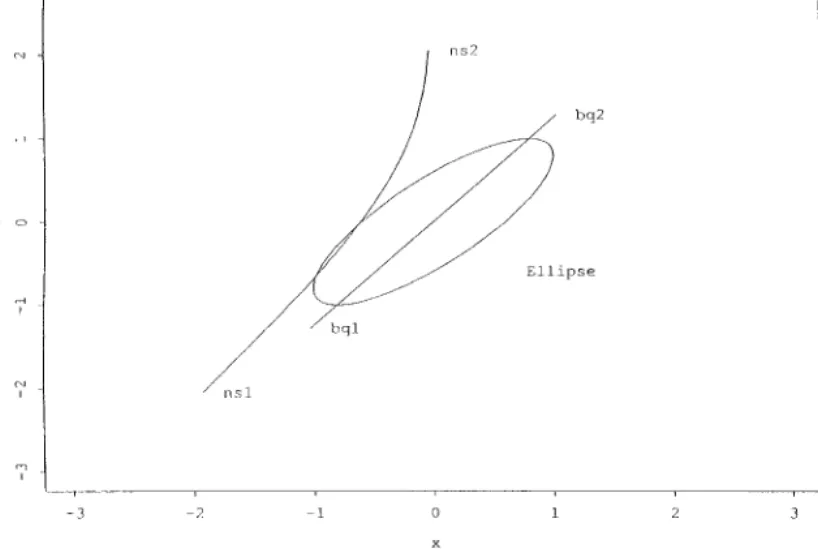
Example _{2. Consider the bivariate normal distribution}

N

1R

S

R

r 1

S2

Figure 1 shows the NS bivariate quantile points (on the curve from ns1 to ns2) and the bivariate quantile points (on the curve from bq1 to bq2) for

r=0.8.

Recall that for any bivariate point x ¥ R2_{, the inner product}

(x − m)Œ (q − m) is the projection of x − m onto the vector (q − m). We require

the following lemma which describes the vector q0 _{that maximizes the}

FIG. 1. The NS bivariate quantile points (on the curve from ns1 to ns2) and the bivariate quantile points (on the curve from bq1 to bq2) for the bivariate normal distribution with means zero, variances one, and correlationr=0.8.

Lemma _{2.4. Suppose that X has mean m and covariance matrix S. Then} var[(X −m)Œ (q − m)] is maximized among all bivariate vectors q satisfying ||q − m||=c for c > 0, by

q0_=cv

2+m, (2.2)

where v2 is the eigenvector corresponding to the largest eigenvalue, say l2, of

S. We can also write

q0_=S1/2

R

0 c

`l2

S

Proof. Equation (2.2) follows from principal component analysis. Since

S1/2_{=P L}1/2_{, we have} S1/2

R

S

R

S

R

S

Lemma 2.4 establishes that if q0_=cv

2+m satisfies the a th probability

cumulation condition, then, var[(X −m)Œ (q0_{− m)] \ var[(X − m)Œ (q − m)]}

for each q satisfying the a th probability cumulation condition and ||q − m||=||q0− m||.

The following theorem establishes conditions under which the bivariate quantiles lie on the principal component axis.

Theorem _{2.5. If Y1 and Y2are independent with symmetric distributions,}

then q0_=S1/2

R

S

That is, q0_{=g(a), the a th bivariate quantile.}

Proof. Since the distribution of Y1 is symmetric about zero, the result

follows from the fact that G2(G−12 (a))=a and P(Y1[0)=1/2. L

Some members of the elliptical family of distributions such as the bivariate normal distribution satisfy the conditions of Theorem 2.5.

2.3. Relationships between NS and Bivariate Median Points

The NS bivariate quantile points and the bivariate quantile points coin-cide when the random variables X₁ and X₂ are independent but not otherwise. Nonetheless, if the distribution of X is symmetric in the sense that X −m and − (X − m) have the same distribution, the bivariate median

point can be expressed as the average of the NS bivariate median point and the SN bivariate median point. This may be useful for avoiding the poten-tial loss of efficiency from having to estimate m and S in order to estimate

the bivariate median point.

Theorem _{2.6. If X has a continuous and symmetric distribution, then the}

bivariate median g(1 2)= 1 2(t( 1 2)+t*( 1 2)), where t*(1 2)=(F g − 1 12 ( 1 4, 1 4), F g − 1 2 ( 1 2))Œ satisfies Fg − 1 2 ( 1 2)=sup{x2: P(X2\x2) \ 1 2} and Fg − 1 12 ( 1 4, 1 4)=sup{x1: P(X1\x1, X2\F g − 1 2 ( 1 2)) \ 1 4} with Fg 12(x1, x2)=P(X1\x1, X2\x2) and F g 2(x2)=P(X2\x2).

Proof. Write Fg − 1

12 (a)=F

g − 1

12 (a/2, a/2). Clearly m is the bivariate

median. We see from the continuity and symmetry of the distribution that

Fg − 1

2 (12)=sup{x2: P(X2\x2) \21}=inf{x2: P(X2[x2) \12}=m2. Again,

by symmetry, F−1

12(12) satisfies P(X1[F−112(12), X2[m2)=14 and F

g − 1

12 (12)

satisfies P(X1\Fg − 112 (12), X2\m2)=14. It follows from the symmetry

prop-erty that t(1

2) and t*( 1

2) are equidistant from m1 and this implies that 1 2(F −1 12(12)+F g − 1 12 (12))=m1. L

3. SAMPLE BIVARIATE QUANTILE POINTS

Let Xi=(X1i, X2i)Πbe a random sample from the distribution with

dis-tribution function F and marginal disdis-tribution functions F1and F2. Let the

density functions of F and F2 be f and f2, respectively. We assume the set

of assumptions listed in the Appendix throughout the rest of this paper. 3.1. Sample NS Bivariate Quantile Points

The empirical marginal distribution function of X2and the empirical left

joint distribution function of X1 and X2 are Fˆ2(x2)=n−1;ni=1I(X2i[x2)

and Fˆ (x1, x2)=n−1;ni=1I(X1i[x1, X2i[x2), respectively.

Definition _{3.1. The sample (a1, a2) th NS bivariate quantile point}

tˆ(a1, a2), the sample a th NS bivariate quantile point tˆ(a), and the sample

NS bivariate median point tˆ(1

2) are defined as in Definition 2.1 with F2 and

F replaced by Fˆ2and Fˆ , respectively.

The sample (a1, a2) NS bivariate quantile has breakdown point

min{a1+a2, 1 − (a1+a2)}. This implies that the breakdown point of the

sample NS bivariate median is 0.5. For comparison, the breakdown points for Weber’s (1909) a1median is 0.5, for Oja’s simplex median is 0, and for

the half space median is 1/3 (see Small (1990)).

To obtain the large sample properties of tˆ(a1, a2), let d1(a1, a2)=

>F2− 1(a1+a2) −. f(F −1 12(a1, a2), x2) dx2andd2(a1, a2)=> F12− 1(a1, a2) −. fx1| x2(x1| F −1 2 (a1

+a2)) dx1, where fx1| x2 is the conditional probability density function of X1

given X2=x2 and F −1 12(a1, a2) satisfies F(F −1 12(a1, a2), F −1 2 (a1+a2))=a1.

Our main result is the following theorem.

Theorem _{3.2. The components of the sample (a1, a2) th NS bivariate}

n1/2_(Fˆ−1 12(a1, a2) − F −1 12(a1, a2)) =d1(a1, a2)−1

53

4

31

2

46

The proof is given in the Appendix.

Corollary _{3.3. The asymptotic distribution of the centered and}

normalized (a1, a2) th NS bivariate quantile n1/2(tˆ(a1, a2) − t(a1, a2))=

n1/2_(Fˆ−1

12(a1, a2) − F−112(a1, a2), Fˆ2−1(a1+a2) − F2−1(a1+a2))Œ is bivariate

nor-mal with mean vector zero and covariance matrix S˜ =(sij, i, j=1, 2), where

s11=d1(a1, a2)−2

51

2

6

1

2

3.2. Sample Bivariate Quantile Points

Put Yi=(Y1i, Y2i)Œ=S−1/2Œ(Xi− mˆ), where S and mˆ represent estimators of

S and m, respectively. The corresponding empirical distribution functions

of Y=(Y1, Y2)Œ and Y2 are Gˆ (y1, y2)=1n; n

i=1I(Y1i[y1, Y2i [y2) and

Gˆ₂( y₂)=n−1_;n

Definition _{3.4. The sample (a1, a2) th bivariate quantile point and the}

sample bivariate median point gˆ(1

2) are defined as in Definition 2.2 with m,

S, G2, and G replaced bymˆ, S, Gˆ2, and Gˆ , respectively.

Arguments similar to those used to prove Theorem 2.4 show that the sample bivariate quantile point is equivariant provided the estimators S andmˆ are equivariant.

We assume that g and g2are continuous, positive, and finite and that g2,

g−

2, g, “g/“y1, and “g/“y2are bounded functions.

Theorem _{3.5. Let (Y}g

1i, Y

g

2i)Œ=S−1/2Œ(Xi− m). Then the sample bivariate

quantile point satisfies

n1/2_(gˆ(a 1, a2) − g(a1, a2))=n1/2(S1/2− S1/2)

R

S

1R

S

R

S2

5

3

4

5

6

6

with s− 1and s − 2the rows of S −1/2Œ_, E˜₂=E(X − m | Yg 2=G −1 2 (a1+a2)), p21=P(Y g 2[G −1 2 (a1+a2) | Y g 1=G −1 12(a1, a2)), p12=P(Y g 1[G −1 12(a1, a2) | Y g 2=G −1 2 (a1+a2)), E˜12=E[(X − m) I(Y g 1[G −1 12(a1, a2) | Y g 2=G −1 2 (a1+a2)], E˜21=E[(X − m) I(Y g 2[G−12 (a1+a2) | Y g 1=G−112(a1, a2)].

3.3. An Estimator of the Bivariate Median Point under Symmetry We showed in Section 2.3 thatg(1

2)= 1 2(t( 1 2)+t*( 1 2)) under symmetry. We

now explore the properties of the estimator of g(1

2) constructed from 1 2(t( 1 2)+t*( 1 2)). Let Fˆg

2(x2)=n−1;ni=1I(X2i\x2) and Fˆ

g 12(x1, x2)=n−1;ni=1I(X1i\x1, X2i\x2). Theorem _{3.6. Let tˆm=}1 2(tˆ*( 1 2)+tˆ( 1 2)) where tˆ*( 1 2) is defined in Theorem 2.6 with Fg 2 and F g 12 replaced by Fˆ g 2 and Fˆ g 12, respectively. Then, if

the distribution of X is symmetric, n1/2_(tˆ

m− m) has the same asymptotic

distribution as that of n1/2_(Fˆ−1

12(1/2) − F−112(1/2), Fˆ2−1(1/2) − F−12 (1/2))Œ in

Corollary 3.3 with a1=a2=14.

The proof of Theorem 3.6 is analogous to that of Theorem 3.5 and so is omitted.

Thus when the bivariate distribution is symmetric, we can obtain a consistent estimator of the bivariate median without having to estimatem

andS.

If we usegˆ(1

2) to estimate g( 1

2), we need to estimate at least S and perhaps

alsom, and the estimates of these quantities affect the efficiency of gˆ(1 2). On

TABLE I

Efficiencies of the Sample Mean X¯ , Sample Bivariate Median gˆ, and tˆmforr=0.2

Estimate s=1 s=3 s=5 s=10 s=15 d=0.1 X¯ 1.000 0.968 0.538 0.171 0.083 gˆ 0.657 0.973 0.962 0.876 0.832 tˆm 0.679 1.000 1.000 1.000 1.000 d=0.2 X¯ 1.000 0.807 0.389 0.110 0.048 gˆ 0.675 0.971 0.950 0.946 0.929 tˆm 0.671 1.000 1.000 1.000 1.000

TABLE II

Efficiencies of the Sample Mean X¯ , Sample Bivariate Median gˆ, and tˆmforr=0.8

Estimate s=1 s=3 s=5 s=10 s=15 d=0.1 X¯ 1.000 0.872 0.512 0.151 0.074 gˆ 0.698 0.933 0.955 0.842 0.853 tˆm 0.725 1.000 1.000 1.000 1.000 d=0.2 X¯ 1.000 0.707 0.334 0.097 0.043 gˆy 0.636 1.000 0.985 0.972 0.969 gˆm 0.679 0.977 1.000 1.000 1.000

the other hand,tˆm does not require estimates of eitherS or m so it may be

more efficient than gˆ(1

2). To explore this possibility, we computed the

asymptotic variances of the three estimators X¯ , gˆ(1

2) (using the sample mean

and variance to estimatem and S, respectively), and tˆm under the bivariate

mixture distribution (1 − d) N

1R

S

R

S2

1R

S

R

S2

and compared their efficiencies. We present the results in Tables I and II in terms of the ratio of the minimum asymptotic variance of the three estima-tors to the asymptotic variance of each estimator so that the efficiency is always less than one. That is, the most efficient estimator has efficiency equal to one.

Not surprisingly, for small s, the sample mean X¯ is the most efficient

estimator. As s increases, tˆm becomes the most efficient estimator. While

tˆmis mostly more efficient thangˆ(12), the improvement in efficiency through

usingtˆmis quite small.

4. QUANTILE CURVES AND OTHER DERIVED QUANTITIES The analogue of the real interval [F−1_(a

1), F−1(a2)] in two dimensions is

a set J(a) whose boundaries can be called bivariate quantile curves. By

analogy to the univariate case, it is most useful to think of J(a) as a set

bounded by two quantile curves. Thus, while we have thought of bivariate quantiles as points in R2_{, for many purposes, it is more natural to think of}

Once we have defined an appropriate set J(a) or equivalently

appropri-ate quantile curves, we can then define the extremes to be the extreme quantile curves (the boundaries of the extreme set J(0, 0,1

2, 1

2)), we can

generalize the interquantile range to the interquantile area which is the area

A(a)=>J(a)dx of J(a), and we can define the trimmed mean to be the

mean over the set J(a), namely m(a)=(>J(a)dF(x))−1>J(a)x dF(x). These

derived quantities are equivariant or not according to whether the quantile curves are equivariant or not, so it is of particular interest to construct equivariant quantile curves.

One simple analogy to the univariate quantile interval is the bivariate quantile parallelogram.

Definition _{4.1. The a=(a1, a2, a3, a4)Πth bivariate quantile}

parallelo-gram is P(a)=

3

R

S

4

Just as we can think of the quantile interval as the intersection of the two intervals [F−1_(a

1), .) and (−., F−1(a2)], with the finite boundaries

defining the quantiles, we can think of the quantile parallelogram as the intersection of the two sets with finite boundaries

C(a1, a2)=boundary

3

R

S

4

3

R

S

4

ifa1, a2[12. (In most practical applications, it will be sensible to have both

arguments equal and hence on the same side of1

2.) The curves C(a1, a2) are

potential quantile curves which we call the quantile parallelogram curves. Definition _{4.2. Thea th quantile parallelogram curve is given by}

C(a)=boundary

3

R

S

1

2

1

24

ifa \1 2and C(a)=boundary

3

R

S

1

2

1

24

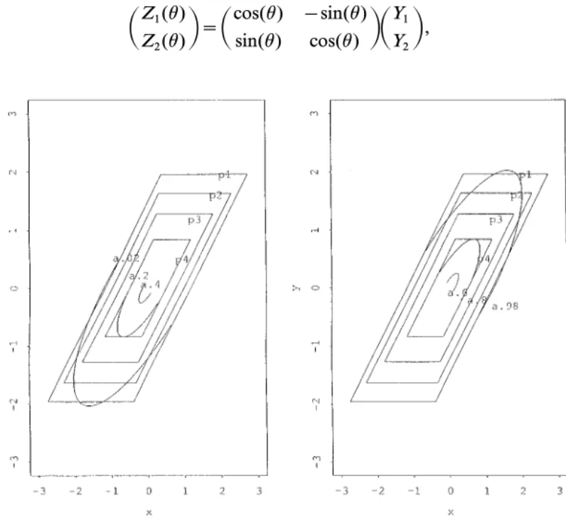
Example _{2 (continued). Consider again the bivariate normal} distribu-tion of Example 2 with r=0.8. Quantile parallelograms for this

distribu-tion are shown in Fig. 2 witha=0.025, 0.05, 0.1, and 0.2 (denoted by p1,

p2, p3, and p4, respectively).

A different approach is to consider defining a bivariate quantile point for each possible rotation of the coordinate system and then rotate the resulting curve back into the original coordinate system. Thus, if we let

R

S

R

SR

S

FIG. 2. The quantile curves fora=0.02, 0.2, and 0.4 (denoted qc.02, qc.2, and qc.4 in (a))

and the quantile curves for a=0.6, 0.8, and 0.98 (denoted qc.6, qc.8 and qc.98 in (b)).

(a) Quantile parallelograms and quantile curves (0 [h [ p). (b) Quantile parallelograms and

we can define the (a1, a2) th NS bivariate quantile point th(a1, a2) for

(Z1(h), Z2(h))Œ. The (a1, a2) th quantile curve is then

S1/2

R

− sin(h) cos(h)

S

h(a1, a2)+m (4.1)

viewed as a function ofh for fixed a1 anda2. (We can define the (a1, a2) th

NS bivariate quantile curve by replacing Y by X and omitting the final renormalization byS1/2_andm.)

If we consider all possible rotations (all possible values ofh), the quantile

curves are closed. (For the bivariate normal distribution, the curves are ellipses in R2_{.) These quantiles reduce to a point in the upper tail and one}

in the lower tail for the univariate case. This is not really what we think of as a univariate quantile. An approach which reduces in the univariate case to the univariate quantile is to consider only half the set of possible rota-tions corresponding to the intersection of the closed curve with the half-plane x2> x1 ifa1+a2>12and with the other half-plane otherwise. In this

case, the quantile curve is defined in the half-plane on either side of the line

x2=−x1. To partition the space R2, we can extend the curve linearly along

the boundary line x2=−x1.

Definition _{4.3. The bivariate quantile curve is the intersection of the} curve defined by (4.1) with the set {(x1, x2)Œ: x2\ − x1} if a >12 and

{(x1, x2)Œ: x2[− x1} if a <12.

Example _{2 (continued). Consider again the bivariate normal} distribu-tion of Example 2 with r=0.8. Figure 2a shows the quantile curves for a=0.02, 0.2, and 0.4 (denoted qc.02, qc.2, and qc.4) and Fig. 2b shows the

quantile curves fora=0.6, 0.8, and 0.98 (denoted qc.6, qc.8, and qc.98).

We can apply the quantile curve approach using the marginal quantile instead of a bivariate quantile point. Of course, the points on the curve then no longer satisfy bivariate probability cumulation conditions. We could also consider using the boundaries of the sets defined by Einmahl and Mason (1992) to define quantile curves but our approach is computa-tionally simpler.

Estimators of the quantile curves and the derived quantities are easily constructed simply by replacing the unknown population quantities by their empirical analogues.

5. EXAMPLES

In this section, we examine the quantiles of two real data sets. In the first example we display the two proposed bivariate quantiles and illustrate the

partitions of the data implied by them. In the second example, we illustrate the use of NS bivariate quantile points as a basis for statistical inference.

Reaven and Miller (1979) measured several variables to compare normal patients and diabetics. Among the variables, the three variables of major interest were X1, glucose intolerance; X2, insulin response to oral glucose;

and X3, insulin resistance. For our bivariate quantile analysis, we consider

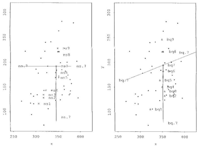
the variables X1 and X2. Figures 3a and 3b show, respectively, the NS

bivariate quantile points tˆ(a), for a=0.1, 0.2, ..., 0.9 (labeled × and

denoted ns1, ..., ns9), and the bivariate quantile pointsgˆ(a) (labeled g and

denoted bq1, ..., bq9). We have also included the observations (labeled · ) and the partitions of the data implied by the NS bivariate quantile point and the bivariate quantile point ata=0.7 (denoted ns.7 and bq.7).

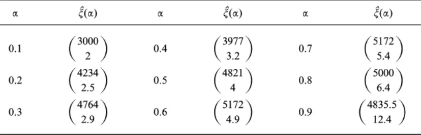
The sales price of rural land depends on many variables, including the closeness of a parcel to transportation facilities. Maddala (1988) gives a sample of size 67 of data on sales prices (per acre) of rural land near Sarasota, Florida, and some other variables. For a bivariate variables

FIG. 3. The NS bivariate quantile points tˆ(a), for a=0.1, 0.2, ..., 0.9 (labeled × and

denoted ns1, ..., ns9 in (a)) and the bivariate quantile pointsgˆ(a) (labeled g and denoted

bq1, ..., bq9 in (b)). We also show the observations (labeled · ) and the partitions of the data implied by the NS bivariate quantile point and the bivariate quantile point ata=0.7 (denoted

ns.7 and bq.7, respectively). (a) Sample NS bivariate quantile points for normal patients. (b) Sample bivariate quantile points for normal patients.

TABLE III Sample NS Bivariate Quantiles

a tˆ(a) a tˆ(a) a tˆ(a)

0.1

R

S

R

S

R

S

R

S

R

S

R

S

R

S

R

S

R

S

analysis, we consider the variables sale price (X1) and distance from the

parcel to the I-75 freeway (X2). To see if these two variables are related, we

could fit a simple linear regression model with X1as the dependent variable

and X2 as the independent variable and then test the significance of the

slope parameter, not to be greater than zero. We can explore the hypothesis informally by examining the NS bivariate quantiles

tˆ(a)=

R

S

12(a/2, a/2) represents the median of the observations (x1i, x2i)Œ

subject to X2i[Fˆ −1

2 (a), there will be a positive relationship between X1

and X2 if Fˆ −1

12(a/2, a/2) decreases as a increases. We display the NS

bi-variate quantiles fora=0.1, 0.2, ..., 0.9 in Table III. Clearly, Fˆ−1

12(a/2, a/2)

does not decrease in a, providing evidence against the hypothesis. Note

that this exploration does not require the assumption of a linear relation-ship between X₁and X₂.

6. HIGHER DIMENSIONS

The bivariate quantile can be extended to higher dimensional observa-tions. Suppose that the random vector X=(X1, X2, ..., Xp)Πhas a location

vector m and positive spread matrix S. Again, let the p-vectors s−

1,

s−

2, ..., s

−

p denote the rows ofS−1/2Œ. We denote the distribution function of

the random variables Xj, ..., Xpby Fj...p(xj, ..., xp). When j=1 we also write

F=F1...p. The (a1, a2, ..., ap)th NS multivariate quantile point is the vector

t(a1, a2, ..., ap)=(F−112 .. p(a1, a2, ..., ap), F−12 .. p(a1+a2, a3, ..., ap), ..., Fp − 1p−1 (a1

F−1 p (a1+a2+ · · · +ap)=inf{xp: Fp(xp) \ a1+a2+ · · · +ap}, F−1 p − 1p(a1+ · · · +ap − 1, ap)=inf{xp − 1: Fp − 1p(xp − 1, F −1 p (a1+a2+ · · · +ap)) \a1+ · · · +ap − 1}, x F−1 23 .. p(a1+a2, a3, ..., ap)=inf{x2: F23 .. p(x2, F−13 .. p(a1+a2+a3, a4, ..., ap), ..., F−1 p (a1+a2+ · · · +ap)) \ a1+a2}, and F−1 12 .. p(a1, a2, ..., ap)=inf{x1: F(x1, F2...p−1 (a1+a2, a3, ..., ap), ..., F−1 p (a1+a2+ · · · +ap)) \ a1}, fora1, a2, ..., ap\0 and a1+a2+ · · · +ap[1.

Fora1, a2, ..., ap\0 and a1+a2+ · · · +ap[1, the vector g(a1, a2, ..., ap)

is an (a1, a2, ..., ap) th multivariate quantile point if

g(a1, a2, ..., ap)=m+S1/2t*(a1, a2, ..., ap), where t*(a1, a2, ..., ap)=(G −1 12 .. p(a1, a2, ..., ap), G −1 23 .. p(a1+a2, a3, ..., ap), ..., G−1 p − 1p(a1+ · · · +ap − 1, ap), G −1 p (a1+a2+ · · · +ap))Œ is the (a1, a2, ..., ap) th

NS multivariate quantile point of Y=S−1/2Œ_{(X − m).}

APPENDIX

Leta1 anda2\0 and a1+a2[1. The following conditions are assumed

to be true for random vector X,mˆ, and S:

(a1) The probability density function f2 and the conditional

proba-bility density function fx1| x2, with x2=F

−1

2 (a1+a2), and their derivatives

are both bounded and bounded away from 0 in neighborhoods of F−12 (a)

and F−1

12(a1, a2), respectively.

(a2) There exists t > 0 such that the probability density function of

(X − m)Œ (sj+d) is uniformly bounded in a neighborhood of H, with

H=G−1

2 (a) if j=2 and H=G−112(a1, a2) if j=1, for ||d|| [ t and the

probability density function of (X −m)Œ (sj+d)(X − m)Œ u((X − m)Œ sj) is

uniformly bounded away from zero for ||u||=1 and ||d|| [ t, for j=1, 2.

(a3) E(((X − m)Œ sj)2||(X − m)||) < . for j=1, 2.

(a4) n1/2_{(mˆ − m)=O}

Proof of Theorem 3.2. The representation of Fˆ−1

2 (a1, a2) can be seen in

Ruppert and Carroll (1980). The first component of the sample NS bivariate quantile point Fˆ−1

12(a1, a2) can be formulated as a solution of the

problem min a C n i=1 (X_1i− a)

1

2

3

4

Then we need to show that

sup ||t1|| [ k, ||t2|| [ kŒ

:

5

6:

Now, (7.1) is bounded above by the two terms

a1 a1+a2 sup ||t2|| [ k

:

:

which is op(1) by the properties of univariate quantiles, and

sup ||t1|| [ k, ||t2|| [ kŒ |S˜(t1, t2) − S˜(0, 0) − {d1(a1, a2) t1 +f₂(F−1 2 (a1+a2)) d2(a1, a2) t2}|, (7.2) where S˜(t1, t2)=n−1/2C n i=1 I(X1i[F−112(a1, a2)+n−1/2t1, X2i[F2−1(a1+a2)+n−1/2t2).

We have E |I{X1i[F−112(a1, a2)+n−1/2t11, X2i[F−12 (a1+a2)+n−1/2t12} − I{X1i[F12−1(a1, a2)+n−1/2t21, X2i[F−12 (a1+a2)+n−1/2t22}| [E |I{X1i [F−112(a1, a2)+n−1/2t11} − I{X1i[F−112(a1, a2)+n−1/2t21}| +E |I{X_2i [F−1 2 (a1+a2)+n−1/2t12} − I{X2i[F2−1(a1+a2)+n−1/2t22}| [M(||t2 1− t 1 1||+||t 2 2− t 1 2||) and, similarly, E sup ||t1− t11|| [ k, ||t2− t12|| [ kŒ |I{X1i[F−112(a1, a2)+n−1/2t1, X2i[F−12 (a1+a2)+n−1/2t2} − I{X1i[F−112(a1, a2)+n−1/2t11, X2i [F−12 (a1+a2)+n−1/2t12}| [C{P(|X1i− F−112(a1, a2)| [ k+kŒ)+P(|X2i− F−12 (a1+a2)| [ k+kŒ)} [CŒ(k+kŒ).

We can apply Lemma 3.2 of Bai and He (1998) to show that (7.2) is op(1)

provided

sup

||t1|| [ k, ||t2|| [ kŒ

||E(S˜(t₁, t₂) − S˜(0, 0)) − {d1(a1, a2) t1

+f2(F−12 (a1+a2)) d2(a1, a2) t2}||=op(1). (7.3)

Using the techniques of Jurecˇkova´ (1984), we can establish both (7.3) and also that n1/2_(Fˆ

12(a1, a2) − F −1

12(a1, a2))=Op(1). Using the fact that

n1/2_(Fˆ−1

2 (a1+a2) − F −1

2 (a1+a2))=Op(1), the theorem then follows.

Proof of Theorem 4.2. The second component of the sample bivariate quantile point Gˆ−1

2 (a) can be formulated as a solution of the minimization

problem min a C n i=1

(Y2i− a)(a − I(Y2i[a)).

By letting F1(t1, t2, t3)=n−1/2 C n i=1 [a − I{(s2+n−1/2t3)Œ (Xi− m) [ G−12 (a) +n−1/2_((s 2+n−1/2t3)Œ t1+n−1/2t2}],

the representation for Gˆ−1

2 (a) follows from:

(a) F1(T1, T2, T3) − F1(0, 0, 0) − g2(G−12 (a))[s

−

2T1+T2− T

−

3E˜c2(a)]=

op(1) for any sequences Tjwith Tj=Op(1).

(b) n1/2_(Gˆ−1 2 (a) − G

−1

2 (a))=Op(1), and

(c) n−1/2_;n

i=1(a − I(Y2i[Gˆ−12 (a))=F1(n1/2(mˆ − m), n1/2(Gˆ−12 (a) −

G−1

2 (a)), n1/2(s2− s2))=op(1).

The proof of the above statements can be derived by similar arguments to those used in the proof in Chen et al. (1999) and is therefore omitted. The proof for Gˆ−1

12(a1, a2) which follows also establishes a more general case.

The first component of the sample bivariate quantile, Gˆ−1

12(a1, a2), is a

solution of the minimization problem min a C n i=1 (Y_1i− a)

1

2

5

6

Then, we want to show that max tj\kj |F˜ (tj) − M˜ (tj)|=op(1). (7.4) Let us denote B(tj)=n−1/2 C n i=1 [I{(s1+n−1/2t4)Œ (Xi− m) [G−1 12(a1, a2)+n−1/2((s1+n−1/2t4)Œ t1+t3), (s2+n−1/2t5)Œ (Xi− m) [G−1 2 (a1+a2)+n−1/2((s2+n−1/2t5)Œ t1+t2)} − I{s− 1(Xi− m) [ G −1 12(a1, a2), s − 2(Xi− m) [ G −1 2 (a1+a2)}].

From the result in the first part of this proof, (7.4) is shown from the fact that sup ||tj|| [ kj |B(tj) − h(tj)|=op(1), (7.5) where h(t_j)=g₁(G−1 12(a1, a2))[ − t − 4E˜21+p21(s − 1t1+t3)] +g₂(G−1 2 (a1+a2))[ − t − 5E˜12+p12(s − 2t1+t2)],

which is implied from the following (see Chen et al. (2001) for analogous proofs), n−1 _C n i=1 E(h˜i(t1j) − h˜i(t2j))2[n−1/2M C 5 j=1 ||t2 j− t1j||, (7.6) with writing B(tj)=n−1/2; n

i=1h˜i(tj) and, fixing t 0 j, E sup ||t1j− t 0 j|| [ k |h˜_i(t0 j− t 1 j)| [ n−1/2Mk for some M > 0. (7.7)

From (7.6), (7.7), and Lemma 3.2 of Bai and He (1999), we have sup

||t0j|| [ k

|F˜ (t0

j) − EF˜ (t0j)|=op(1).

To complete the proof, we still need to show that sup ||t0j|| [ k |EF˜ (t0 j) − M˜ (t 0 j)|=o(1). (7.8) Write EF˜ (t0 j)= a1 a1+a2 n1/2_EI((s 2+n−1/2t 0 5)Œ (X − m) [ G −1 2 (a1+a2) +n−1/2_((s 2+n−1/2t05)Œ t01+t20)) − n1/2EI((s1+n−1/2t04)Œ (X − m) [G−1 12(a1, a2)+n−1/2((s1+n−1/2t04)Œ t01+t03)), (s2+n−1/2t05)Œ (X − m) [G−1 2 (a1+a2)+n−1/2((s2+n−1/2t05)Œ t01+t02)) =H1+H2. We denote variables Yg 1=Y1− G−112(a1, a2) and Y g 2=Y2− G−12 (a1+a2). Let Z1=t0Œ4(X − m), Z2=t0Œ5(X − m), d1=n−1/2((s1+n−1/2t04)Œ t01+t03), and d2= n−1/2_((s

2+n−1/2t05)Œ t01+t02). Then we can see that the two terms in the

|H₂+g₁(G−1 12(a1+a2))[ − t 0Œ 4E˜21+p21(s − 1t 0 1+t 0 3)] +g₂(G−1 2 (a1, a2))[ − t 0Œ 5E˜12+p12(s − 2t 0 1+t 0 2)]|

:

:

are all bounded by Mn−1/2_{which establishes (7.8).}

Finally, as in Ruppert and Carroll (1980),

n−1/2 _C n i=1

3

4

and, by an analogous argument to that given in Jurecˇkova´ (1977, Lemma 5.2), fore > 0 there exists k > 0, a > 0, and N such that

P

1

:

1

2

:

2

for n \ N. These two results together establish that

n1/2_(Gˆ−1

12(a1, a2) − G −1

12(a1, a2))=Op(1)

and the representation for Gˆ−1

12(a1+a2) follows.

REFERENCES

D. F. Andrews and A. M. Herzberg, ‘‘Dta,’’ Springer-Verlag, New York, 1985.

Z.-D. Bai and X. He, Asymptotic distributions of the maximal depth estimators for regression and multivariate location, Ann. Statist. 27 (1999), 1616–1637.

V. Barnett, The ordering of multivariate data (with discussion), J. Roy. Statist. Soc. A 139 (1976), 318–354.

V. Barnett and T. Lewis, ‘‘Outliers in Statistical Data,’’ Wiley, New York, 1994. J. Breckling and R. Chambers, M-quantiles, Biometrika 75 (1988), 761–771.

P. Chaudhuri, On a geometric notion of quantiles for multivariate data, J. Amer. Statist.

Assoc. 91 (1996), 862–872.

L.-A. Chen, A. H. Welsh, and W. Chan, Linear winsorized means for the linear regression model, Statist. Sinica 11 (2001), 147–172.

J. H. J. Einhmahl and D. Mason, Generalized quantile process, Ann. Statist. 20 (1992), 1062–1078.

J. Jureckova, Asymptotic relation of M-estimates and R-estimates in linear regression model,

Ann. Math. Statist. 5 (1977), 464–472.

J. Jureckova, Regression quantiles and trimmed least squares estimator under general design,

V. I. Koltchinskii, M-estimation, convexity and quantiles, Ann. Statist. 25 (1997), 435–477. A. Kudo, The extreme value in a multivariate normal sample, Mem. Fac. Sci. Kyushu Univ.

(A) (1957), 143–156.

R. Y. Liu, On a notion of simplicial depth, Proc. Nat. Acad. Sci. USA 18 (1988), 1732–1734. R. Y. Liu, On a notion of data depth based on random simplices, Ann. Statist. 18 (1990),

405–414.

G. S. Maddala, ‘‘Introduction to Econometrics,’’ Macmillan, New York, 1988.

R. A. Maller, Normality of trimmed means in higher dimensions, Ann. Probab. 16 (1988), 1608–1622.

H. Oja, Descriptive statistics for multivariate distributions, Statist. Probab. Lett. 1 (1983), 327–332.

G. M. Reaven and R. G. Miller, An attempt to define the nature of chemical diabets using a multidimensional analysis, Diabetologia 16 (1979), 17–24.

D. Ruppert and R. J. Carroll, Trimmed least squares estimation in the linear model, J. Amer.

Statist. Assoc. 75 (1980), 828–838.

M. Sibuya, Bivariate extreme statistics, Ann. Inst. Statist. Math., Tokyo 11 (1960), 195–210. C. G. Small, A survey of multidimensional medians, Internat. Statist. Rev. 58 (1990), 273–277. R. L. Smith, J. A. Tawn, and H. K. Yuen, Statistics of multivariate extremes, Internat. Statist.

Rev. 58 (1990), 47–58.

A. Weber, ‘‘Über den Standort der Industrien,’’ Tubingen; ‘‘Alfred Weber’s Theory of Location of Industries,’’ University of Chicago Press, Chicago, 1909.