Dynamic spatial modeling approach for estimation of internal phosphorus load

@

Pergamon 01998ElsmierScienceLtd.Allrizhtsreserved

PII: S0043-1354(97)00190-5

Printedin &eat Britain 0043-1354/98S19.00+ 0.00

DYNAMIC SPATIAL MODELING APPROACH FOR

ESTIMATION OF INTERNAL PHOSPHORUS LOAD

JEHNG-JUNG KAO@*, WANG-LONG LIN and CHENG-HSIEH TSAI Instituteof EnvironmentalEngineering,NationalChiaoTung University,75 Po-AiStreet,Hsinchu,

Taiwan30039,China

(ReceivedSeptember1996;acceptedin revisedform June 1997)

Abstract-The effectof the pollutionloadgeneratedinternallyfroma reservoiron the effectivenessof an eutrophicationcontrolplan is significantand has gainedincreasingattentionreeently.Accurate estimationof theinternalloadisdifficultbecauseofits spatialandtemporalvariation.A procedureusing a dynamicspatialmodelingapproachis proposedto improvethe estimation.A case studyof Posan off-streamreservoirisdescribedto demonstratetheimplemementationoftheprocedurefordatacollection and modelpreparation,fieldsamplingplanningand investigation,laboratoryanalysisfor phosphorus releasingrates,modelintegrationof AGNPSand WASP,calibrationand verificationof the integrated model,and the internalloadestimation.Theprocedureis expectedto provideappropriatetemporaland spatialphosphorusinternalloadestimationforan off-streamreservoir.Q 1998ElsevierScienceLtd.All rightsreserved

Key words—internalload, nonpoint-sourcepollution, dynamic modeling,water-qualitymodel, phosphorusreleasingrate, modelintegration,off-streamreservoir

INTRODUCTION

Eutrophication control for a reservoir or lake has gained increasing attention recently. Contamination generated from the upstream development and human activities introduces a significantamount of nutrients into a reservoir and, thus, accelerates the eutrophication process, spoils the public water resources, and requires costly remediations. Phos-phorus and nitrogen are major limit factors of eutrophication. From previousfieldinvestigationsfor reservoireutrophication in Taiwan (WUet al., 1992), available nitrogen is, however, much more than available phosphorus in a reservoir,and phosphorus is, therefore, generallyconsideredas the indicator of eutrophication.

There are two sources of phosphorus for a reservoir or lake: external and internal loads. External loads come from the point or nonpoint-source pollutants and are carried by runoff from storm events. Internal loads are mostly from the phosphorusreleasedfrom benthos of the water body. Phosphorus in the water body is presented in both solid and liquid phases. Solid-phase phosphorus is mostly attached on the suspendedparticles of point or nonpoint-sourcepollutants. Some of the particles, after being brought into the water body, settle and become parts of benthic sediment. The

phytoplank-*Authorto whomcorrespondenceshouldbe addressed ~el: +886-3-5731869,Fax: +886-3-5725958,E-mail: jjkao@green.ev.nctu.edu.tw].

ton dead residuals of benthos contributes also some solid-phase phosphorus in water bodies (Jacoby etal., 1982).Soluble phosphorus is dissolved from the phosphorus adsorbed on the suspendedparticles or released from benthos.

Particles and phosphorus could be released from benthos through physical, chemical, or biological disturbancesand processes(Holdren and Armstrong, 1980;Rossi and Premazzi, 1991;Dillon and Evans, 1993). Such internal loads contribute a significant amount of phosphorus nutrients in some seasons for a water body, evenwhenexternal pollution inputs are extremelylimited(Freedman and Canale, 1977;Rossi and Premazzi, 1991).Jacoby etal. (1982)estimated that the internal phosphorus released from benthic sediment is approximately 20-500/0of that from external loads. It should be noted that the sediment physiochemical characteristics vary seasonally and cause phosphorus adsorption and resorption phenomena (Jacoby etal., 1982;Istvanovics, 1988). In some seasons, phosphorus is adsorbed instead of released from the sediment. In addition to the seasonal change, geographic location as well as different portions of a reservoir would characterize different phosphorus releasing rates (Jacobyet al., 1982). Previous local studies for eutrophication were mostly focused on the water quality and external loads only, and the internal load was rarely explored, especiallyfor an off-stream reservoir, due to sampling and modeling difficulties, although the importance of the internal load estimation had been stated in previous research (Wu et al.,

48 Jehng-JungKaoetal.

1992).The present study was, therefore, initiated to explore an adequate procedure for estimating the internal load.

Three methods for internal load estimation are generally adopted: (1) using representative sampling data to determinethe releasingrate, (2)usinga simple mass balance calculation to estimate the overall releasing rate, and (3) applying a statistical method. These methods, however, can not practically reveal the spatial distribution and dynamic temporal variation in detail. A dynamic spatial modeling approach with field sampling data was, therefore, explored in this study for simulating the dynamic behavior of the benthic sediment adsorption and resorption of phosphorus.

The procedure adopted in this work for phos-phorus internal loading estimation and simulation consistsof fivemajor steps:data collectionand model preparation; sampling planning and field investi-gation; laboratory analysis for phosphorus releasing rates; model integration, calibration, verificationand simulation; and internal load estimation. In the followingsections,these steps are described.The case study of an off-streamreservoir is then presented to exemplify the proposed procedure as well as to demonstrate the manipulation for model integration, multiple step calibration, etc.

DATACOLLECTIONANDMODELINGPREPARATION

The study area

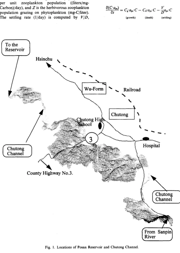
Some areas in Taiwan lack a suitable location to build a general reservoir and have to apply an off-stream method to re-direct the stream flow to a reservoirthat is not on the stream network. This kind of off-stream reservoir differs from the general one for pollution load estimation. Pollution loads from the watershed of the reservoiras well as the loads on the inflow channel must be analyzed simultaneously and, therefore, increase the complexity of modeling simulation. The study area was the Posan off-stream reservoir located in Hsinchu, Taiwain, China. The location of the reservoirand inflowchannel, Chutong Channel, is illustrated in Fig. 1. The reservoiris used for the supplyof public drinkingwater. It has an area of 60.2ha with effective storage of up to 5,350,000m3.Chutong channel is the inflowchannel that transfers water from Sapin river to the reservoir and irrigates agricultural areas within Chutong watershed. The channel is 13.36km in length, of which 6635m is closed channel and 6501m is open channel. The water quality of total phosphorusin the reservoir is around 20-40 ppb. Based on Carlson (1977)standard, it is in eutrophy status and requires attention for water-qualitycontrol. The main sources of nutrients comefrom the water transferred from the Chutong channel, external sources within the watershed for the reservoir, and the internal load within the reservoir itself.

Before the internal loading can be properly simulated, external loads must be estimated. Unfor-tunately, currently no single model is appropriate to be utilized for simulating both external and internal loads. Two separate models, AGNPS (Young etal., 1987) and WASP (Ambrose et al., 1993), were selected, therefore, for external and internal loading simulations, respectively.The two models are briefly described below, while detailed information for the models is available in the original documents. AGNPS

AGNPS is a physical-basedmodel developed for evaluating upstream land erosions and water quality to meet the requirement of US federal regulations. It is a grid-based model for single storm-event simulation. Watershed are divided into numerous rectangle grids which are not necessary of the same size. Hydrology, soil erosion, nutrient, and sediment movementare computed for each model grid and for inter-grid transport. Runoff data are determined by the SCS curve (Wischmeierand Smith, 1978)or unit hydrographymethods. Upland and channel erosion from a storm event is determined primarily based on the Universal Soil Loss Equation (Wischmeierand Smith, 1978).Total nitrogen (TN), total phosphorus (TP), and chemical oxygen demand are the water quality parameters analyzed in the model.

WASP

WASP is a dynamic compartment model devel-oped by US EPA (Ambroseet al., 1993)that can simulate the water quality of water column and underlying benthos for an aquatic system using the finite segmentationmethod. A water body is divided into layers of segments.With a proper segmentation, the model is applicable for a three-dimensional dynamic simulation. The model can analyze phos-phorus and seven other water-quality parameters. This study concentrated mainly on the phytoplank-ton, organic, and inorganic phosphorus. The phytoplankton growth,death, settling,and mineraliz-ation are considered by the model. The internal loading is determined by phosphorus releasing rates, settling rates, transfer coefficients,and concentration gradient betweenthe sediment and bulk water phase. Important equations related to phytoplankton and the phosphorus cycle are listed below.

Phytoplankton kinetics. Chlorophyll-a is used as the aggregated variable for phytoplankton, and the major kinetics equation is expressed below:

g =

(Cg– c, –

C,)c

where C is the phytoplankton concentration (mg-C/ liter), C, is the specificgrowth rate (l/day),cd is death rate (l/day), and C, is the settling rate (l/day). The specific growth rate is computed by CmT,L.N, where Cm is the maximum specific growth rate at optimum light and nutrients, T, is the temperature

adjustment factor, L is the light limitation factor, where Vis the net settling velocity of phytoplankton and N is the nutrient limitation factor as a (m/day) and D is the depth of water column of model function of dissolved inorganic phosphorus and segment.

nitrogen. Death rate (l/day) is determined by The phosphorus cycle. The phosphorus cycle is E,+ D,, + G.Z, where E, is the temperature cor- mainly simulated by the followingthree equations for rected endogenous respiration rate, DP, is the phytoplankton, organic and inorganic. phosporus, death rate caused by parasitization or toxic respectively:

materials, G is the grazing rate on phytoplankton per unit zooplankton population

((liters/mg-Carbon)/day), and Z is the herbivorouszooplankton

a(cww) cg.ap.c–

Cd.aw.C – ~aFC”c

v

population grazing on phytoplankton (mg-C/liter). —=

at

The settling rate (l/day) is computed by V/D, (Srowth) (death) (settling)

fiia

F

Wu-Form

“)

\ _{~ Railroad} \ \ mChutong ~_s

‘y“2+2”

f“+::&,-

Hospital

Jehng-JungKaoet al.

Reservojboundary

N

(to w

inlet

from Chutqng Channel)

I I ._{I I}

t

*

m

Ikm

■+ preliminary sampling Iocati

+ Regular sampling locations

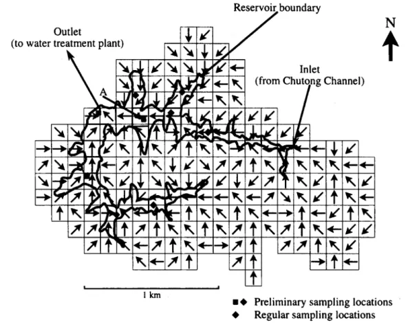
Fig. 2. AGNPS/WASPsegmentationfor Posan watershed.

aop

()

— = cd.up.fOp.c

_at

– Pm.e;;

20.&c

.OP

(death) (mineralization) L’..(1 ‘fdo,) Op — D (settling)

()

~=

Cd.a.(1‘f.p)c + pm’&-20

&

Op

(death) (mineralization)

– Cg.aw.C (growth) whereawis phosphorusto carbon ratio (mg-P/mg-C), OP isthe organicphosphorusconcentration,Pmisthe dissolvedorganic phosphorus mineralizationat 20”C

(l/day), j&, is the fraction of dead and respired phytoplankton recycled to the organic phosphorus pool, (1~is temperature correction coefficientforP., h is the half saturation constant for phytoplankton limitation of phosphorus recycle (mg-C/liter); Vois the organic matter settlingvelocity(m/day),~d.Pis the fraction dissolvedorganic phosphorus, and1P isthe inorganic phosphorus concentration.

,ons

Benthic simulation. The benthos and water exchange phenomenon for phosphorus is simulated by the followingthree equations:

~ = d.~@&20ww”f.p”C– dop+)~p-zo.fdop.zp (algaldecomposition) (mineralization)

aop

— = d~~4K:20qdl

_at

–A,)C + d~P@~J’Of&ZP

(dgd

decomposition) (mineralization)

whered,n.is the anaerobic algal decomposition rate (l/day), I%.,is the temperature correction coefficient ford.”,, doPis the organic phosphorus decomposition rate (l/day), OOPis the temperature correction coefficientfordoP;~ is the fluxbetweenwaste benthic segment j and water segmenti, E is the diffusive exchangecoefficient,Db isthe benthic layer depth,P] is the phosphorus (ZP or OP) concentration of benthic segmentj; Piisthe phosphorus(IP or OP) concentration of water segmenti,and~ andj are the dissolved fractions.

Modeling segmentation

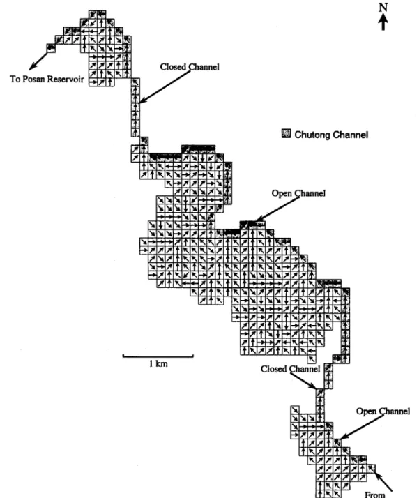
For applying AGNPS and WASP, the watershed and water body must be divided into small model elements that are called grids for AGNPS and segments for WASP. The criteria for grid division include terrain variation, soil types, land uses, hydrological characteristics, etc. Smaller grids de-scribe geographical data more precisely, but more computation time and data preparation effort are required. As a compromise, the grid size of 120m x 120m was used in this study. The grid

To PosanReservoir

Ikm

division with drainage pattern for Chutong and Posan reservoir watersheds are shown in Figs 2 and 3, respectively.For Chutong channel, it was assumed that the open channel accepted and transported most external pollutants from storm runoff and, therefore, the portion of closed channels was excluded for modeling simulation.

Criteria for WASP segmentation for a water body include (1) minimizing the segment volume differ-ences to diminish the possible numerical dispersion, (2) selecting appropriate size that can express the representativeaverage of water-qualityconcentration

N

4

❑

ChutongChannel

52 Jehng-JungKaoetal. distribution, and (3) requiring vertical divisionif the

stratification exists in the water profile. Moreover, and more important for this study, proper segmenta-tion to coordinate with grids used by AGNPS can significantlyreduce the difficultyof exchangingdata between the models and, therefore, facilitate the model integration task. Finally, the boundariesof the upper layer of segments were made as close to the grid boundaries for AGNPS. The water body was divided into two layers because a distinct stratifica-tion existed at 8 m deep. The final segmentastratifica-tion of the water profile was divided into 46 segments, of which 26 were for the upper layer, as shown by the bold lines in Fig. 2, and 20 for the lower layer. With the layer for benthic segmentsbelow the lower water segments, a total of 66 segmentswere used. Data collection and model parameter preparation

For external loading simulation by AGNPS, data collected in a previous study (Kaoet al., 1994)were utilized. Numerous parameters are required for applyingWASP. Data for WASP parameters mainly came from three sources:(1) experimentallaboratory analysis under aerobic and marginal anaerobic conditions for possibleranges of organic phosphorus releasingrates, (2)theoreticalestimation, and (3)data cited in previous similar studies (e.g. Bowieet al., 1985;Thomann and Mueller, 1987).

SAMPLINGPLANNINGANDFIELDINVESTIGATION

The field sampling plan included two stages of preliminary and regular samplings and three major parts of water, benthic sediment, and watershed. Preliminary sampling was implemented to realize water quality and pollution distribution for selecting appropriate regular sampling points. Water in the

reservoir profile was sampled for both upper and lower layers. Two meters below the water surface and

1–2m above the sedimentsurfacewere sampled.Ten sampling points selected for this stage are shown in Fig. 2. Phosphate-relatedand other parameters for all samples were analyzed. Five of the points, as shown in Fig. 2, were finally selected for weekly (water column) and bi-weekly (benthic sediment) regular sampling. Benthic sediment was collected using a gravity corer dropped from a boat. Water-quality parameters for pore water were analyzed similar to those for the upper or lower water column. Sediment was used for laboratory analysisdescribedin the next sectionfor estimation of releasingrates. Settlingmass were collectedby severalsets of catchers. Each set of catchers were placed and lined up vertically within the water column;catchers wereput about 3 m apart. External load sampling for Chutong and Posan watersheds during two events were implemented. This task was difficultbecause it was hard to predict when a representative storm event would occur and sampling had to be done within a short period for collecting effective samples for analyzing the first

flush pollutant load distribution, peak flow, and water-qualityparameters. Sampleswere collected for >10 min during the first hour of the event, and few samples were collected after then. Sampling points were selected primarily based on land uses and geographical terrain and, of course, the manpower available to this research. One or two representative points were selected for each major land use.

LABORATORYANALYSISFORPHOSPHORUS

RELEASINGRATES

The transfer mechanism between water bulk and the benthic sediment includes soluble phosphorus released from the solid phase of the sediment and physical movement of soluble phosphorus from the sediment to water phase. The phosphorus releasing rate may be affected by dissolvedoxygen (DO), pH (Ku et al., 1978),ox-reduction potential (Andersen,

1982), microorganism (Jacoby et al., 1982), and transport mechanism (Freedman and Canale, 1977; Holdren and Armstrong, 1980). In this study, no significant pH variation was observed from field sampling.

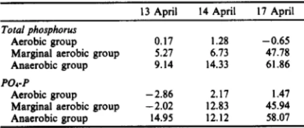
Originally,it was thought that the sediment phase was under the anaerobic condition. From the field sampling results, however, it was under marginal anaerobic condition with low DO. The possible reason is that the reservoiris not deep enoughto keep oxygen transfer away. Experiments were, therefore, set into two groups, one in marginal anaerobic and one in aerobic condition. Nitrogen was aerated to maintain, the marginal anaerobic condition under 1ppm DO level, when the aerobic set was kept around 6 ppm DO. All the experiences were prosecuted on a round rack with column tubes directly removed from the gravity corer. The release rates of ortho-phosphorusand TP for typical samples in April 1994are listed in Table 1. In general, the release rates obtained from the anaerobic set were higher than those from the aerobic set. Few resorption results in the aerobic set and adsorption results in the anaerobic set were observed. These results indicate that other factors in addition to DO were important for determining the release rate. The study of the mechanism is, however, beyond the scope of this research and is currently under exploration.

Table 1. Phosphorusrelease rates ((mg/m2)/day)for sampling locationA

13Amil 14Auril 17ADIil

Totalphosphorus Aerobicgroup MarginalaerobicSroup Anaerobicgroup PO,-P Aerobicgxoup Marginal aerobic group Anaerobic erouo 0.17 1.28 –0.65 5.27 6.73 47.78 9.14 14.33 61.86 –2.86 2.17 1.47 –2.02 12.83 45.94 14.95 12.12 58.07

53

MODEL INTEGRATION, CALIBRATION,

VERIFICATION ANDSIMULATION

External loading simulation by AGNPS

The modelingsimulation was implementedfor the period of 26 January to 25 April 1994.During this period, there were 19 significant storm events. The model verification for the AGNPS model were implemented in two steps: (1) verification of the modeling result with benthic sedimentchange within 3 years, and (2) verification with data sampled in storm events. Although AGNPS is a physical-based model for which the calibration step is generallynot implemented, many parameters used by AGNPS were collected from USA cases and might not be appropriate for the local characteristics. For example, the fertilizingpattern in Taiwan is different from that in the USA, and rainfall intensityeffectsfor soil erosion differssignificantlyfrom that in the USA according to previous local research. Some model parameters were, therefore, adjusted based on local characteristics of the watersheds. The verificationof the model is done first for sediment because detailed sedimentation data are available for the years of 1986-1988.After model parameters were specified from various geographical maps and field investi-gation, the model was implementedfor 84 significant storm events during the 3 years. This verificationwas detailed by Kao et af. (1994). The total arrival amount of sediment from these events is approxi-mately 17,783t, that is about 8Z0/0of the actual change monitored during the 3 years. Possible reasons for the differenceinclude that (1) the 3-years data were monitored after the reservoir was established and no investigation was carried out for the initial collapse of reservoir rims during the construction period; (2) gully sources were not adequate simulated because of no research available to verify the applicability of the AGNPS suggested parameters for local areas; and (3) events were simulated discretely instead of continuously due to the limitation of AGNPS for a singleevent only. The result is, however,good enough whencompared with related local external (or nonpoint-source) loading research results. Model verification was then im-plemented further for sampled data from field investigation. Parameters related to sediment were not adjusted in this step, and parameters such as fertilizing level that related to water quality were adjusted based on values obtained from some previous local research.

Integration of AGNPS and WASP

Other than the grid/segment division, some other problems must be resolved in order to integrate both models. For water-quality parameters for phosphorus and nitrogen, WASP simulates ortho-phosphate, organic phosphorus, inorganic phos-phorus, ammonia nitrogen, nitrate and organic nitrogen, while AGNPS handles only soluble

phosphorus, phosphorus adsorbed in sediment, and TP. These nutrient parameters are not compatible for both models. Some conversion factors are, thus, determined based on hydrography using a time-weighted approach. Water-quality parameter frac-tions in runoff of the sampled storm events for ortho-phosphate in the soluble phosphorus and the fractions of ammonia nitrogen, nitrate, and organic nitrogen in the TN were computed. Unfortunately, the fractions were not constants, and a flow-weighted averagemethod based on the hydrographywas used to determine the factors. The conversionratios, for the Posan and {Chutong}watershed, are PO,-P:organic-P:TP = 0.743:0.24:1 {0.836:0.12:1} and NH,-N: NO,-NH,-N:TN = 0.191:0.388:0.423

{0.212:0.328:0.46}. The ratios for PO,-P and organic-P to TP are not summed up to one and are not adjusted because some poly-phosphorus or complex and laboratory analysis errors may exist. Other than the determination of the ratios, many intermediate computer programs were written to process the output filescreated by the two models to facilitate the integration and result presentation. Internal loading simulation by WASP

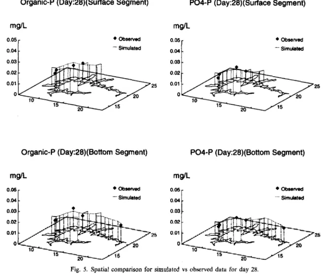
The model built by WASP was first calibrated for water volume changes. Consideringtime and spatial factors, segment volumes were adjusted to get the results similar to the real storage volume change during a period of 3 months. For water-quality simulation, model parameters for non-phosphorus items were calibrated before adjusting model parameters for phosphorus-related items. External loads were obtained from the AGNPS model. The model was implemented dynamically for the cali-bration period between26 January to 21 March 1994 and the verificationperiod of 21 March to 25 April 1994.Figure 4 compares the simulated and sampled results for both calibration (days 1–55) and verification periods (days 55–90) for each segment where field samples are available. Segmentsindexed larger than 26 are bottom water segments. Figure 5 showsa similar comparison for spatial differencefor day 28 during the calibration period. The simulated concentration for ortho-phosphate, organic-P, and other parameters are acceptablewhencompared with the fieldsampleddata, although fewover-estimations and under-estimations are observed.

INTERNALLOADESTIMATION

Finally, the internal phosphorus load of the reservoirwas estimated usingthe establisheddynamic model. The internal load was determined by the following equation based on dynamic modeling results:

Internal load

Jehng-JungKaoetal. segmemr40 0.07

-m

Slmulmed. 04savea . # + o.m 3 . . . & 0.02 “. 0.01 . . o.07r m 15 ₍ 0.07 S4gnwfll1 0.03 sml&ata:.

k22-1

simulated. Obwlved. ~:. ~ 0.0s $ “. 0.02 “ . 0.01 0 . . . . 0 102030atiwmw70 so so 100 o~ 0 1020 so 4ti30011 703030100 s62mmlr40 0.07, ( 0.07, Sagmard 15 0.07, -1

& :

4.

I

0.020.02

‘

0.01!, simdmed. Obsemud . ‘ .

“1

o~ 0 1020304005001170 so w 100 o~0 102020M*!wll 70 Sll 90100 0.07, -= t 0.07 segment 12 0.03 s-: -0.03

i’_

0.04 $::

M.

0.01 . _. . ,. 0 . 0 1020so @Mw&l 70 so 30100 o~ 0 1020 w ati300fl 708030100 007 -= 0.06

m

simubrad-$

0.0s Olwaned . -0.04

1!

0.03 . i 0,02 “. 0.01 . 0.07, -35 1 0.07 Sagmmrt12 L Sinruktad. C4wmfed. & a i 0.02 _. O.a? _{. .} . 0.01 . . . o“ 0 1020 so 4ccygl 7030 m f 0.06

L

$=:

‘i’

-0.05 - 0.04 + * 0.03 130.a? . 0 . . . O.of . “. . . > o 0 102030 ati~wcl 70 so 30 m D o -~= 007 0.06

L

s=:

$

0.03 _ 0.04 a 0.03

6

0.02 “. . 0.01 .’ o 0 1020 so atimm$l 70 so 90‘ SWmeIIt42 0.07. 0.07 sagmmrt20

E

shmMal-Obwnwd . ~;: -. + 0.03 Eocz “ o . . 0.01 _. . . 0 0 1020 so 4ooywlJ 70 Bo 30 IW 0,07 -~

D

slmulmed-Obwlwd . ~;: n

!

0.03 0.02 . 0.01‘ “ . 0.07 -=

L

Slmubtad. CtMrwd . g;; a

I/

0.03 0.02 0.01 . . . . , SqIrnmt42 0.07 m Simulnmd. CbIelvd. g;; ]:: , “ 0,01 . “ “ “ “ “ “ o~ 0 102030 am500(l 703030 Iw

Organic-P(Day:28)(SurfaceSegment) P04-P (Day:28)(SutfaceSegment) mg/L mg/L 0.05 I + ob~.g~~ _0.05 1 + c)b~~~ 0.04 -“”SimulaWd 0.04 ‘“””Simulatad 0.03 - 0.03 -0.02 - 0.02 -0.01 - ₂₅ 0.01 - ₂₅ 0 0 10 10 15 20 15 20 Organic-P(Day:28)(BottomSegment) P04-P (Day:28)(Bottom mg/L mg/L 0.05 [ + ob~~~ _0.05 0.04 ‘- Simulated 0.04 [ Segment) ●obs,sw~ . ~imuktd 0.03 0,0s 0.02 0.02 0.01 ₂₅ 0.01 ₂₆ 0 0

Fig. 5. Spatial comparison for simulated vs observeddata for day 28.

where k is the number of time intervals, n is the number of WASP segments,vi,, and vi,t-Iare the volume of segment i at timetand t – 1, respectively, PI,,and pi,,-, is the TP concentration of segmentiat time tand t – 1, respectively, b is the numbe~ of boundary segments, w],,is the external load entered into boundary segment j at time t, and po~,, is boundary loss (including output) of boundary boundary loss (including output) of boundary segmentj at timet.For convenience,time intervals were all set to be equal to 1 day, although the model time tand t-1,respectively, b is the number of boundary segments, Wj,,is the external load entered into boundary segment j at time t,and p~j,f is

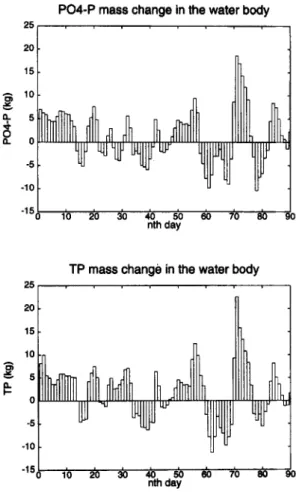
computation interval is smaller. The first term for mass changed within the water body is computed based on results shown in Fig. 6. The second term, listed as (A) and (B) in Table 2 for external loads and output loss, is computed based on results obtained from the AGNPS modeling output. The internal loads determined with this dynamic modeling approach are 41.74 and 1.59kg for the calibration and verification periods.

CONCLUSIONS

h-tthis article, a case study for the Posan off-stream reservoir is described to exemplify the utilization of

Table 2. Estimation of total phosphorus internal loads (kg) External load

output (Posan+ Chutong) Net change Internal load

(A) (B) (c) (A) + (C)– (B) Simplemassbalance Calibration period 77.94 147.26 81.38 12.06 Verificationperiod 32.13 87.38 48.20 –7.05 Entire period 110.07 234.64 129.58 5.01 Dynamicmodeling(from Fig. 6) Calibration period 77.94 147.26 111.06 41.74 Verificationperiod 32.13 87.38 56.84 1.59 Entire period 110.07 234.64 167.90 42.33

Jehng-JungKaoet al. P04-P masschangeinthewaterbody 25 20 15 g 10 $: -5 -lo -15 nth day TP masschangeinthewaterbody -15 ,0 I 20 S040 50 W 70 so so nth day

Fig. 6.Phosphorus mass change in the water body (computed based on dynamic spatial modelingresults).

the proposed internal loading estimation procedure using a dynamic spatial model. The integration approach proposed for combining AGNPS and WASP makes it possible to simulate both internal and external loadings simultaneously with proper segmentation and determination of water-quality conversion ratios. The multiple step calibration and verification procedure demonstrated for the case study reduces the complexity of calibrating the numerous parameters of both models at the same time. The internal load estimation by the dynamic modeling approach with field investigation and laboratory analysis provides detailed variation. In addition to the overalltrend, the spatial and temporal distribution of the results and parameters are available with the dynamic modeling approach, and these results are expectedto provide insight into the

system and, therefore, facilitate the planning for an efficient water-quality control strategy. The pro-cedure, although it is primarily designed for the off-stream reservoir, is also applicable for other similar internal load estimation of a reservoiror lake. Additional research, however, is necessary to explore further and to enhance the modeling estimation procedure. For example, the mechanism of phosphorus releasing rates for local reservoirs,

appropriate model parameters that are applicable for local areas, a long-termcomprehensivesamplingplan for external loads, internal loads, and model parameters, and a single model for simulating both internal and external loads need to be studied in more detail, although research for these issuesis expensive and manpower-intensive.

Acknowledgements—Theauthors thank National Science Council, Taiwan, Republic of China, for providingpartial financial support (Grant No. NSC 82-O41O-E-OO9-382). They acknowledgekind assistancefrom Mr R. B. Ambrose of US EPA. Many undergraduate students from the Civil Engineering and Applied Chemistry Department of National Chiao Tung University who helped in field investigationsand laboratory analyses are greatly appreci-ated, although it is impossibleto list all of them.

REFERENCES

Ambrose R. B., Wool T. A. and Martin J. L. (1993)The water quality analysis simulation program, WASP5: model documentation and input dataset. Environmental Research Laboratory, US EPA, Athens, GA.

AndersenJ. M. (1982)Effectof nitrate concentrationin lake water on phosphate releasefrom the sediment.W’at.Res.

16, 1119-1126.

BowieG. L., Mills W. B., Porcela D. B., CampbellC. L., Pagenkoph J. R., Rupp G. L., Johnson K. M., Chan P. W. H. and Gherini S. A. (1985)Rates, constants, and kinetics formulations in surface water quality modeling, EPA/600/3-85/040,2nd edn. US EPA.

Carlson R. E. (1977)A tropic state indexfor lakes. Limrrol. Oceanogr.22, 361-369.

Dillon P. J. and Evans H. E. (1993) A comparison of phosphorus retention from mass balance and sediment core calculations.Wat.Res. 27, 65%668.

Freedman P. L. and Canale R. P. (1977)Nutrient release from anaerobic sediments.ASCE J.Enuiron.Engng 1M(EE2),233-244.

Holdren G. C. and Armstrong D. E. (1980) Factors affecting phosphorus release from intact lake sediment cores. Environ.Sri. Technol.14(1), 79-87.

Istvanovics V. (1988) Seasonal variation of phosphorus release from the sediments of shallow lake Bakaton (Hungary).War. Res.22, 1473-1481.

Jacoby J. M., Lynch D. D., Welch E. B. and Perkins M. A. (1982)Internal phosphorusloadingin a shalloweutrophic lake. Wat. Res. 16, 911-919.

Kao J.-J., Tsai M. C. and Bau S. F. (1994)Developmentof analysis models for total mass load based discharge programs (I), NSC 81-O41O-EOO9-382.Report to ROC National ScienceCouncil, Taipei, Taiwan, R.O.C. Ku W. C., Digiano F. A. and Feng T. H. (1978)Factors

affecting phosphate adsorption equilibria in Iake sedi-ments. War. Res. 12, 1069-1074.

Rossi G. and Premazzi G. (1991)Delay in lake recovery caused by internal loading. Wat. Res. 25, 567–575. Thomann R. V. and Mueller J. A. (1987) Principlesof

SurfaceWater QualityModelingand Control.Harper &

Row, New York.

Wischmeier W. H. and Smith D. D. (1978) Predicting

Rainfall Erosion Losses, Arg. Handbook 537. US

Department of Agriculture, Washington, DC.

Wu S.-C.,Wang,M.-S.and ChenS.-Y.(1992)Mass balance and control strategy for reservoirs in Taiwan. Report to ROC EPA, (in Chinese),Taipei, Taiwan, R.O.C. Young R. A., Onstad C. A., Bosch D. D. and Anderson

W. P. (1987) AGNPS, agricultural non-point source pollution model. USDA-ARS, Morris, MN.