低成本高效率內容適應性可變長度編碼器之設計

(1)

國立交通大學

電子工程學系電子研究所碩士班

碩士論文

低成本高效率內容適應性可變長度編碼器之設計

A Low Cost and High Throughput CAVLC Encoder

Design

學生 :吳秈璟

指導教授 :張添烜博士

(2)

低成本高效率內容適應性可變長度編碼器之設計

A Low Cost and High Throughput CAVLC Encoder

Design

研究生 : 吳秈璟 Student

:

Sian-Jing

Wu

指導教授 : 張添烜博士 Advisor

:

Dr.

Tian-Sheuan

Chang

國立交通大學

電子工程學系電子研究所碩士班

碩士論文

A Thesis

Submitted to Institute of Electronics

College of Electrical Engineering and Computer Science National Chiao Tung University

in Partial Fulfillment of the Requirements for Degree of Master of Science

in

Electronic Engineering July 2007

(3)

低成本高效率內容適應性可變長度編碼器之設計

學生 : 吳秈璟

指導教授 : 張添烜博士

國立交通大學

電子工程學系電子研究所碩士班

摘要

本論文提出一個低成本高效率的內容適應性可變長度編碼器。本論文的動機是為了補償編碼區塊樣式先決的低效能以達到高效率，使得我們所提出的內容適應性可變長度編碼器能支援每秒處理30張1080p畫面。此外，在如此高效率之下，我們必須維持少量的邏輯閘。編碼區塊樣式先決能跳過一些零方塊的編碼流程來提高效率。然而，我們的統計數據指出有大量的零係數無法被編碼區塊樣式先決偵測到，使得許多的週期數被浪費在零係數。在我們的設計裡，除了採用編碼區塊樣式先決，我們還使用可以直接對非零係數作編碼的新奇架構，以避免花費時間在零係數：零方塊碼字表與非零索引表。當我們所提出的內容適應性可變長度編碼器在一個週期內讀取一個方塊的所有係數時，非零索引表同時記錄那些係數是非零的。然後非零索引表會分辦這個方塊是否為全零。假如這方塊是全零，零方塊碼字表可以在不用跑完整套內容適應性可變長度編碼流程的情況下，直接產生這個方塊的全部碼字。另一方面，如果這個方塊含有至少一個非零係數，非零索引表使用組合電路找出非零係數的位置，使得零係數被忽略。再者，

(4)

當非零索引表鎖定一個非零係數時，這個非零係數的碼字會直接被連接到H.264/AVC的位元串流。因此，我們不需要額外的緩衝存儲器來儲存這個非零係數，使得少量的邏輯閘被消耗。最後，基於聯華電子點一三微米製程，我們所提出的設計在145 MHz的工作時脈之下，消耗了9.03 K個邏輯閘，且可支援每秒處理30張1080p的畫面。和其它的設計相較之下，我們可以節省61%的邏輯閘與29%的週期數。

(5)

A Low Cost and High Throughput CAVLC Encoder

Design

Student : Sian-Jing Wu

Advisor : Dr. Tian-Sheuan Chang

Institute of Electronics

National Chiao Tung University

ABSTRACT

This thesis proposes a low cost and high throughput CAVLC encoder. The motivation is to compensate the inefficiency of CBP Look-Ahead to achieve higher throughput such that the proposed CAVLC encoder can support 1080p at 30 fps. Moreover, under such high throughput, we must keep logic gate count low. CBP Look-Ahead can skip encoding flow of some zero blocks such that throughput can be improved. However, our statistics show that abundant zero coefficients cannot be detected by CBP Look-Ahead such that many cycle counts are wasted on the zero coefficients. In our design, we use novel direct significance encoding architectures, as well as CBP Look-Ahead, to avoid spending time on zero coefficients: Zero-block Codeword Table and Nonzero Index Table.

Nonzero Index Table concurrently records which coefficients are significant while the proposed CAVLC encoder is reading all coefficients of a block in one cycle. Then Nonzero

(6)

Codeword Table will generate the overall codeword of the block without going through the whole CAVLC encoding flow. On the other hand, if the block consists of at least one significant coefficient, Nonzero Index Table uses combinational circuits to locate significant coefficients such that zero coefficients are ignored. In addition, while Nonzero Index Table is aiming for a significant coefficient, the codeword of the significant coefficient can be directly concatenated into the H.264/AVC bit-stream. Hence, we do not need additional buffers to store the significant coefficient such that small logic gate count is consumed.

Eventually, based on 0.13um UMC technology, the proposed design can support 1080p at 30 fps while consuming 9.03 K gate count at 145 MHz. Compared with other designs, we can reduce 61% logic gate count and 29% cycle count.

(7)

誌謝

首先，要感謝我的指導教授－張添烜博士，在張教授的指導之下，我學習到作研究正確的方法與態度。此外，張教授所提供的優良實驗室環境和軟硬體資源，使得我的研究能夠順利進行，才有這本論文的誕生。同時也要謝謝我的口試委員們，交大研發長李鎮宜教授、清大電機陳永昌教授，感謝各位在百忙之中抽空前來指導我，各位教授的寶貴意見讓本論文得以更加完備。接著，我要感謝實驗室的夥伴。謝謝林佑昆學長，領導我們走向晶片下線成功的坦途，學長在晶片下線期間努力建構與維護測試平台，並時常與我交流驗證的心得，使我的驗證能夠順利進行。謝謝李國龍學長和張彥中學長，給予課程和研究上的指導，讓研究得以順利進行。謝謝李得瑋同學、林嘉俊同學和郭子筠同學，你們所設計的高效能演算法，得以讓我們團隊的晶片達到下線的規格要求。也謝謝張瑋城學弟和戴瑋呈學弟，在晶片下線期間，分擔部分的驗證工作與後段佈局流程。此外，要謝謝廖英澤同學，宇晟，宗憲，景竹等學弟，你們的幫忙讓我的實驗室生活能順利渡過。所有的一切，都是我在交大的寶貴回憶。最後，我要感謝我的家人們，你們的默默支持，是我能夠完成學業的最大動力。在此，我謹把這篇論文獻給所有愛我與我愛的人。

(8)

List of Figures

Fig. 1 Block Diagram of an H.264/AVC encoder [2] ... 3

Fig. 2 Division of Y component in a macro-block ... 5

Fig. 3 Separation of DC and AC for Y ... 6

Fig. 4 Division of U component in a macro-block ... 6

Fig. 5 Separation of DC and AC for U ... 6

Fig. 6 Separation of DC and AC for V ... 7

Fig. 7 Division of an Intra_16x16 macro-block ... 7

Fig. 8 Division of a non-Intra_16x16 macro-block... 8

Fig. 9 Four groups of an Intra_16x16 macro-block ... 9

Fig. 10 Four groups of a non_Intra16x16 macro-block ... 10

Fig. 11 Three adjacent macro-blocks in Y-frame... 12

Fig. 12 Three adjacent macro-blocks in U-frame... 13

Fig. 13 Three adjacent macro-blocks in V-frame ... 13

Fig. 14 A LUMA_DC sub-block ... 14

Fig. 15 Zigzag scan order ... 15

Fig. 16 Structure of Array_Coeff... 15

Fig. 17 Structure of H.264/AVC bit-stream... 16

Fig. 18 Scanning for a LUMA_AC sub-block ... 23

Fig. 19 Scanning for a CHROMA_DC sub-block... 23

Fig. 20 A group of four LUMA sub-blocks ... 25

Fig. 21 Average number of nonzero coefficients per NS4B sub-block ... 27

Fig. 22 Percentage of NSZB in all-zero sub-blocks ... 28

Fig. 23 Partial system architecture of an H.264/AVC encoder... 29

Fig. 24 Organization of Luma SRAM ... 31

Fig. 25 Y sub-blocks of a macro-block... 31

Fig. 26 Organization of a word in Luma SRAM ... 31

Fig. 27 The coefficients of a LUMA sub-block... 32

Fig. 28 The coefficients of a LUMA_AC sub-block ... 32

Fig. 29 Organization of Chroma SRAM ... 32

Fig. 30 U and V sub-blocks of a macro-block... 33

Fig. 31 Organization of one word in Chroma SRAM ... 33

Fig. 32 Coefficients of a CHROMA_AC sub-block ... 34

Fig. 33 Organization of LDC Register ... 34

(11)

Fig. 35 Organization of CDCU Register ... 35

Fig. 36 Coefficients of a CHROMA_DC sub-block ... 35

Fig. 37 Architecture of CBP Generator ... 36

Fig. 38 Sub-block Index of each sub-blocks in a macro-block ... 37

Fig. 39 Architecture of Entropy SRAM Interface ... 38

Fig. 40 BlkIdx_cur for each sub-block of an Intra_16x16 macro-block ... 39

Fig. 41 BlkIdx_cur for each sub-block of a non-Intra_16x16 macro-block... 39

Fig. 42 Timing schedule of fetch_step_cur ... 40

Fig. 43 Architecture of Exp-Golomb Coding Unit ... 41

Fig. 44 Structure of Exp-Golomb codeword ... 42

Fig. 45 Input and Output ports of Bit-stream Packer ... 45

Fig. 46 Architecture of Bit-stream Packer ... 45

Fig. 47 Structure of mux_word... 46

Fig. 48 Structure of residual_word_cur ... 46

Fig. 49 Updating of residual_word_cur by left_shifter when longer_than_31 is low... 47

Fig. 50 Updating of bitstream_cur by right_shifter... 48

Fig. 51 Usage of TwoByteBuf_cur... 49

Fig. 52 Example for case 1 ... 50

Fig. 53 Encoding flow of the proposed CAVLC encoder... 51

Fig. 54 Input Buffer and Nonzero Index Table... 52

Fig. 55 Nonzero Index Table for an all-zero sub-block... 52

Fig. 56 Coefficient at index 7 is being encoded ... 53

Fig. 57 Coefficient at index 4 is being encoded ... 53

Fig. 58 Architecture of the proposed CAVLC encoder ... 55

Fig. 59 Structure of Input Buffer and Nonzero Index Table... 56

Fig. 60 Start index and stop index with Nonzero Index Table ... 57

Fig. 61 Zero-block Codeword Table... 57

Fig. 62 Updating for Nonzero Index Table... 58

Fig. 63 Coefficients of a LUMA sub-block ... 59

Fig. 64 Loading of Input Buffer and determination of Nonzero Index Table ... 61

Fig. 65 State of Nonzero Index Table at 4th cycle... 61

Fig. 66 Determination of TotalCoeff by Nonzero Index Table... 62

Fig. 67 Determination of total_zeros... 62

Fig. 68 Determination of TrailingOnes ... 63

Fig. 70 Determination and concatenation of run_before... 64

(12)

Fig. 74 Generation of level codeword ... 67

Fig. 81 Generation of total_zeros codeword ... 70

Fig. 82 State of Nonzero Index Table at 3rd cycle for NSZB ... 71

Fig. 83 Determination of an all-zero sub-block... 72

Fig. 84 Two adjacent rows in a frame... 73

Fig. 85 Organization of sram_nonzero for QCIF ... 74

Fig. 86 Structure of sram_nonzero address ... 74

Fig. 87 Mapping relation between sub-blocks and sram_nonzero for a macro-block ... 75

Fig. 88 Timing schedule of sram_nonzero ... 75

Fig. 89 Current macro-block in a QCIF frame ... 77

Fig. 90 Timing schedule for encoding a NAZ sub-block ... 78

Fig. 91 Timing schedule for encoding of an NSZB sub-block... 79

Fig. 92 Timing schedule for encoding of a CS sub-block ... 80

Fig. 93 Average encoding cycles per sub-block ... 81

Fig. 94 Average encoding cycles per macro-block... 82

Fig. 95 Average number of macro-blocks encoded per cycle... 83

Fig. 96 Architecture of Huang [6] ... 85

Fig. 97 Architecture of Chen [3]... 86

Fig. 98 Architecture of Kim [4] ... 87

Fig. 99 Architecture of Chien [13] ... 88

Fig. 100 Architecture of Lai [14]... 89

(13)

List of Tables

TABLE 1 Definition of the coded block pattern for chrominance part [1] ... 10

TABLE 2 coeff_token mapping to TotalCoeff and TrailingOnes [1] ... 17

TABLE 3 total_zeros tables for LUMA, LUMA_DC, LUMA_AC, CHROMA_AC [1]... 21

TABLE 4 Tables for run_before [1] ... 22

TABLE 5 total_zeros tables for CHROMA_DC [1] ... 24

TABLE 6 Simulation setting ... 26

TABLE 7 Structure of Exp-Golomb Code Table [1] ... 41

TABLE 8 Exp-Golomb Code Table in explicit form [1] ... 42

TABLE 9 Assignment of syntax element to codeNum for signed Exp-Golomb [1] ... 42

TABLE 10 Assignment of codeNum to values of CBP [1] ... 43

TABLE 11 Read and write address of sram_nonzero for a sub-block ... 75

TABLE 12 Definition of variable “x” ... 78

TABLE 13 Total cycle counts for CS, NSZB and NAZ... 80

TABLE 14 Requirement of 1080 HD... 83

TABLE 15 Gate count profile of the propose CAVLC encoder ... 84

TABLE 16 On-chip memory requirement of the proposed CAVLC encoder ... 84

TABLE 17 Comparison with other CAVLC encoder designs ... 84

TABLE 18 Definition of serial numbers for zero-skipping methods ... 85

(14)

Chapter 1. Introduction

1.1 Motivation

H.264/AVC [1] is the latest standard for video coding. H.264/AVC is the result of the collaboration between the ISO/IEC Moving Picture Experts Group and the ITU-T Video Coding Experts Group [2]. H.264/AVC is designed to address a large range of applications, such as storage, entertainment, multimedia short message, videophone, videoconference, HDTV broadcasting, and Internet streaming. Compared to previous video coding standards, H.264/AVC can achieve 50% bit-rate reduction under the same quality [10]. The better compression efficiency results from innovative coding tools such as multiple reference frames, variable block size motion estimation, and in-loop de-blocking filter [3].

The essence of H.264/AVC is block-based motion estimation transform coding [3]. For H.264/AVC Baseline profile, context-based adaptive variable length coding (CAVLC) is used to encode quantized transform coefficients of the residual images [2]. Compared with entropy coders of previous standards, CAVLC removes more statistical redundancy by switching VLC tables according to previously transmitted symbols [2]. However, coding is not started until syntax elements are extracted by scanning all coefficients of a block such that throughput is very low [3]. To support high-end applications such as 1080p at 30 fps, we must improve throughput of CAVLC encoder.

H.264/AVC specification stipulates that some all-zero blocks can be skipped according to the coded block pattern (CBP) [1]. For example, Chen [3] uses CBP Look-Ahead to improve throughput. However, our statistics show abundant zero coefficients are not covered

(15)

by the CBP. Therefore, we propose two zero-skipping methods to avoid wasting cycles on zero coefficients such that throughput is improved. The resulting architecture not only has a high throughput but also consumes small area.

1.2 Organization of thesis

This thesis is organized as follows. In Chapter 2, we present the algorithm of CAVLC in H.264/AVC. Chapter 3 presents the proposed design with the two throughput enhancement methods. Moreover, we present related statistics to prove that the methods are necessary. Chapter 4 presents simulation results, implementation results, and comparison with other designs. Chapter 5 concludes this thesis.

(16)

Chapter 2. Overview of CAVLC in

H.264/AVC

2.1 Overview of an H.264/AVC

encoder

Fig. 1 shows the block diagram of an H.264/AVC encoder. An input frame is processed in units of a macro-block [16]. The data flow in Fig. 1 can be divided into the following three steps:

Macro-block of Input Frame Signal

+

Intra-Frame Prediction Macro-block Compensated Prediction Motion Estimation Reference Frame Memory

+

Transform Quantize Prediction Error Signal Quantized Coefficients Entropy Coding Motion Vector Intra/Inter H.264 Bit-stream Prediction Signal Inverse Trans. Inverse Quant. Reconstructed Macro-block

(17)

1. First, we calculate the prediction signal of the macro-block. In general, there are two prediction modes: Intra and Inter. In Intra mode, the prediction signal is calculated according to pixels in the current frame, which have been encoded, reconstructed and stored into Reference Frame Memory. In Inter mode, we use Motion Estimation to estimate the motion vectors, which refer to the corresponding position of the macro-block in an already transmitted (to decoder) frame stored in Reference Frame Memory [2]. Then the prediction signal is generated by Macro-block Compensated Prediction. Note that the motion vectors must be encoded into H.264/AVC bit-stream by Entropy Coding.

2. Second, we subtract the prediction signal from the macro-block to obtain the prediction error signal. Then the prediction error signal is transformed and quantized to generate quantized coefficients, which is compressed into H.264/AVC bit-stream by Entropy Coding. H.264/AVC has two major entropy coding tools: CAVLC for the Baseline Profile and CABAC for the High Profile [1].

3. Third, the quantized coefficients are inverse quantized, inverse transformed, and added to the prediction signal. The result is the reconstructed macro-block which is stored into Reference Frame Memory in order to calculate the prediction signal of the future macro-block.

2.2 Overview of block types

2.2.1 Partitions of a macro-block

As mentioned in section 2.1, Inter mode or Intra mode finds prediction signal of a macro-block [2]. The residual data is obtained by subtracting the prediction signal from the macro-block. Then we apply transform matrices on the residual data to obtain so-called

(18)

quantized transform coefficients [2]. The coefficients of a macro-block can be divided into three components as follows: luminance Y, chrominance U, and chrominance V. The component Y comprises 16 by 16 coefficients. The component U comprises 8 by 8 coefficients, and the component V does, too.

The main purpose of CAVLC is to encode the coefficients. Before encoded by CAVLC, the three components of a macro-block are individually divided into several smaller blocks. For the component Y, we divide it into sixteen 4x4 sub-blocks, as Fig. 2 shows. Each of the sixteen sub-blocks has a DC coefficient. If Intra_16x16 [1] is the prediction mode of the macro-block, we separate the DC coefficients to form another 4x4 sub-block, as Fig. 3 shows.

(19)

Fig. 3 Separation of DC and AC for Y

The component U is divided into four 4x4 sub-blocks, as Fig. 4 shows. Each of the four 4x4 sub-blocks has a DC coefficient. No matter which prediction mode the macro-block uses, we separate the DC coefficients to form another 2x2 sub-block, as Fig. 5 shows. V and U use the identical scheme of partition, as Fig. 6 shows.

Fig. 4 Division of U component in a macro-block

(20)

Fig. 6 Separation of DC and AC for V

In conclusion, macro-blocks have only two types in point of CAVLC. First, an Intra_16x16 macro-block is divided as Fig. 7 shows. Sub-blocks “0”-“16” represent Y, “17” and “19”-“22” represent U, and the remaining sub-blocks represent V. The numbers represent the order in which the sub-blocks are encoded by CAVLC [1].

1 2 5 6 3 4 7 8 9 10 13 14 11 12 15 16 19 20 21 22 23 24 25 26 17 18 0

Fig. 7 Division of an Intra_16x16 macro-block

Second, a non-Intra_16x16 macro-block is divided as Fig. 8 shows. Sub-blocks “0”-“15” represent Y, “16” and “18”-“21” represent U, and the remaining sub-blocks represent V. The numbers in Fig. 8 and Fig. 7 have the same meaning.

(21)

0

1

4

5

2

3

6

7

18

19

20

21

22

23

24

25

8

9

12

13

10

11

14

15

16

17

Fig. 8 Division of a non-Intra_16x16 macro-block

2.2.2 The five sub-block types

After a macro-block is divided into several sub-blocks, the sub-blocks are individually encoded by CAVLC in order as mentioned in section 2.2.1. The sub-blocks are divided into five types [9]. For every type the flow of CAVLC is similar but little different. The first type is LUMA_DC referring to sub-block “0” in Fig. 7. LUMA_DC comprises 16 coefficients. The second type is LUMA_AC referring to sub-blocks “1”-“16” in Fig. 7. Each LUMA_AC sub-block comprises 15 coefficients. The third type is CHROMA_DC referring to sub-blocks “17”-“18” in Fig. 7. Each CHROMA_DC sub-block comprises four coefficients. In Fig. 8 sub-blocks “16” and “17” are also CHROMA_DC. The fourth type is CHROMA_AC referring to sub-blocks “19”-“26” in Fig. 7. Each CHROMA_AC comprises 15 coefficients. Sub-blocks “18”-“25” of Fig. 8 are also classified as CHROMA_AC. The final type is LUMA referring to sub-blocks “0”-“15” in Fig. 8. A LUMA comprises 16 coefficients.

In conclusion, an Intra_16x16 macro-block comprises one sub-block of LUMA_DC, sixteen sub-blocks of LUMA_AC, two sub-blocks of CHROMA_DC, and eight sub-blocks of

(22)

two sub-blocks of CHROMA_DC, and eight sub-blocks of CHROMA_AC.

2.2.3 Coded block pattern

The coded block pattern is a syntax element in H.264/AVC [1]. Every macro-block has a coded block pattern which comprises six bits. The lower four bits represent the component Y and the upper two bits represent U and V. We use it to indicate which sub-blocks comprise only zero coefficients.

For an Intra_16x16 macro-block, we present the definition of the coded block pattern below. The 16 LUMA_AC sub-blocks are divided into four groups, as Fig. 9 shows.

group_0 group_1

group_2 group_3

Fig. 9 Four groups of an Intra_16x16 macro-block

Each group comprises four LUMA_AC sub-blocks. The 0th bit (LSB) of the coded block pattern, corresponds to group_0, the 1st bit corresponds to group_1, and so on. If all coefficients of some group are zero, its corresponding bit is zero. Bit “1” means that the corresponding group comprises at least one nonzero coefficient. As for U and V, the upper two bits are defined as TABLE 1.

(23)

TABLE 1 Definition of the coded block pattern for chrominance part [1]

CodedBlockPatternChroma Description

0 All chroma transform coefficient levels are equal to 0.

1 One or more chroma DC transform coefficient levels are non-zero. All chroma AC transform coefficient levels are equal to 0.

2 Zero or more chroma DC transform coefficient levels are non-zero valued. One or more chroma AC transform coefficient levels are non-zero valued.

Only three combinations of the 5th (MSB) and 4th bit are possible, and we describe the combinations in detail as follows:

1. “00” means that every sub-block is all-zero, including two CHROMA_DC sub-blocks and eight CHROMA_AC sub-blocks.

2. “01” means that either CHROMA_DC sub-block comprises at least one nonzero coefficient but each CHROMA_AC sub-block is all-zero.

3. “10” means that at least one nonzero coefficient is among the eight CHROMA_AC sub-blocks.

For a non-Intra_16x16 macro-block, we present the definition of the coded block pattern below. The sixteen LUMA sub-blocks are divided into four groups as Fig. 10 shows.

group_0 group_1

group_2 group_3

(24)

Each group comprises four LUMA sub-blocks. The 0th bit (LSB) corresponds to group_0, the 1st bit corresponds to group_1, and so on. If group_0 consists of only zero coefficients, the 0th bit is zero. The 0th bit is one means that group_0 comprises at least one nonzero coefficient. For the remaining three groups, the meaning of their corresponding bits in the coded block pattern is identical with group_0. The definition for the U and V is identical with an Intra_16x16 macro-block.

We describe how H.264/AVC specification skips sub-blocks according to the coded block pattern below. Because LUMA_DC has no relation to the coded block pattern, even an all-zero LUMA_DC sub-block must be encoded by CAVLC. As for LUMA, CHROMA_DC, and CHROMA_AC, CAVLC can ignore the sub-block as long as the coded block pattern indicates that the sub-block is all-zero. As for LUMA_AC, skip condition is defined as Eq. 1 shows [1] [9]. blocks -sub LUMA_AC sixteen all encodes CAVLC else blocks -sub LUMA_AC sixteen all ignores CAVLC d0) 4' 0] : (CBP[3 if == Eq. 1

In conclusion, all sub-block types except LUMA_DC have relation to the coded block pattern. We can check the coded block pattern to determine whether CAVLC can skip a sub-block to save cycle counts.

2.2.4 Neighbor

sub-blocks

In the flow of CAVLC, every sub-block type except CHROMA_DC needs neighbor information [9]. The information comes from the sub-blocks neighboring to the left and to the

(25)

top of the current one. We define the neighbor sub-blocks for the four sub-block types, including LUMA, LUMA_AC, LUMA_DC, and CHROMA_AC.

For convenience of explanation, a frame is divided into three parts which respectively represent Y, U, and V. We refer to the three parts as Y-frame, U-frame, and V-frame respectively. A macro-block comprises 16 sub-blocks in Y-frame, as Fig. 11 shows.

0

1

4

5

2

3

6

7

8

9

12

13

10

11

14

15

0

1

4

5

2

3

6

7

8

9

12

13

10

11

14

15

0

1

4

5

2

3

6

7

8

9

12

13

10

11

14

15

mb_0 mb_1 mb_2

Fig. 11 Three adjacent macro-blocks in Y-frame

For an Intra_16x16 macro-block the sixteen sub-blocks are LUMA_AC. The sixteen sub-blocks of a non-Intra_16x16 macro-block are LUMA. For “12” of mb_2 in Fig. 11, the left neighbor is “9” and the top neighbor is “6”. Some sub-blocks are on the border of a macro-block such as “2” of mb_2, so their neighbor may reside in a different macro-block. For example, the left neighbor of “2” in mb_2 is “7” of mb_1. In a frame, some macro-blocks are Intra_16x16 and some are not, so the neighbor of LUMA may be LUMA_AC. Moreover, some sub-blocks falls on the edge of a frame such that their neighbors may be not available. As for a LUMA_DC sub-block, for example, we assume mb_2 is Intra_16x16; The

(26)

LUMA_DC sub-block and “0” have the identical neighbors.

A macro-block comprises four CHROMA_AC sub-blocks in U-frame, as Fig. 12 shows. The neighbors are the sub-blocks neighboring to the left and to the top of the current sub-block. For example, in mb_2 the left neighbor of “3” is “2”, and the top neighbor is “1”. If a sub-block is on the border of a macro-block such as “2” of mb_2, its neighbors may be in another macro-block. As for a macro-block on the border of a frame, some sub-blocks’ neighbors may be not available.

0

1

2

3

0

1

2

3

0

1

2

3

mb_0 mb_1 mb_2

Fig. 12 Three adjacent macro-blocks in U-frame

A macro-block comprises four CHROMA_AC sub-blocks in V-frame, as Fig. 13 shows. V-frame and U-frame have the identical explanation for neighbors.

0

1

2

3

0

1

2

3

0

1

2

3

mb_0 mb_1 mb_2

(27)

2.3 Flow of CAVLC in H.264/AVC

A sub-block is a coding unit of CAVLC. We describe the flow of CAVLC for each sub-block type below.

2.3.1 Encoding flow of LUMA_DC

A LUMA_DC sub-block comprises sixteen coefficients as Fig. 14 shows [11]. The coefficients are scanned in zigzag scan order, as Fig. 15 shows [1]. Then the coefficients are mapped to a 1-D array, Array_Coeff, as Fig. 16 shows.

0

3 -1

0

0 -1

1

0

1

0

(28)

0 1 5 6 2 4 7 12 3 8 11 13 9 10 14 15

Fig. 15 Zigzag scan order

index Array_Coeff 0 0 1 3 2 0 3 1 4 -1 5 -1 6 0 7 1 index Array_Coeff 8 0 9 0 10 0 11 0 12 0 13 0 14 0 15 0

Fig. 16 Structure of Array_Coeff

We analyze Array_Coeff to obtain syntax elements as follows [9]:

1. TotalCoeff 2. TrailingOnes 3. Trailing_one_sign_flag 4. Level 5. Total_zeros 6. Run_before

TotalCoeff is the number of nonzero coefficients in Array_Coeff. TrailingOnes means the number of trailing ones (T1s). To define trailing ones, we scan the coefficients in Array_Coeff from index “15” one by one until the occurrence of a nonzero coefficient whose magnitude is greater than one. If we find a coefficient with magnitude equal to one, the coefficient is so-called trailing one. In H.264/AVC the maximum of TrailingOnes is three such that

(29)

Array_Coeff[3] is not classified as a trailing one. H.264/AVC combines TotalCoeff and TrailingOnes into Coeff_token, an H.264/AVC syntax element [1]. Each trailing one has a corresponding trailing_one_sign_flag which comprises only one bit. If the trailing one is negative, its trailing_one_sign_flag is equal to one. A zero trailing_one_sign_flag means that the corresponding trailing one is positive. A level refers to the nonzero coefficient which is not a trailing one. Each nonzero coefficient has a corresponding run_before which is the number of consecutive zeros before the nonzero coefficient in Array_Coeff. For example, the run_before of Array_Coeff[7] is one and that of Array_Coeff[4] is zero. Finally, total_zeros is the sum of all run_before.

After all syntax elements are obtained, we encode them in numerical order as follows [9]: 1. Coeff_token 2. Trailing_one_sign_flags 3. Levels 4. Total_zeros 5. Run_befores

Therefore, the structure of H.264/AVC bit-stream is as Fig. 17 shows.

Coeff_token trailing_one _sign_flags levels total_zeros run_befores

Fig. 17 Structure of H.264/AVC bit-stream

(30)

TABLE 2 coeff_token mapping to TotalCoeff and TrailingOnes [1] TrailingOnes ( coeff_token ) TotalCoeff ( coeff_token ) 0 <= nC < 2 2 <= nC < 4 4 <= nC < 8 8 <= nC nC = = -1 0 0 1 11 1111 0000 11 01 0 1 0001 01 0010 11 0011 11 0000 00 0001 11 1 1 01 10 1110 0000 01 1 0 2 0000 0111 0001 11 0010 11 0001 00 0001 00 1 2 0001 00 0011 1 0111 1 0001 01 0001 10 2 2 001 011 1101 0001 10 001 0 3 0000 0011 1 0000 111 0010 00 0010 00 0000 11 1 3 0000 0110 0010 10 0110 0 0010 01 0000 011 2 3 0000 101 0010 01 0111 0 0010 10 0000 010 3 3 0001 1 0101 1100 0010 11 0001 01 0 4 0000 0001 11 0000 0111 0001 111 0011 00 0000 10 1 4 0000 0011 0 0001 10 0101 0 0011 01 0000 0011 2 4 0000 0101 0001 01 0101 1 0011 10 0000 0010 3 4 0000 11 0100 1011 0011 11 0000 000 0 5 0000 0000 111 0000 0100 0001 011 0100 00 - 1 5 0000 0001 10 0000 110 0100 0 0100 01 - 2 5 0000 0010 1 0000 101 0100 1 0100 10 - 3 5 0000 100 0011 0 1010 0100 11 - 0 6 0000 0000 0111 1 0000 0011 1 0001 001 0101 00 - 1 6 0000 0000 110 0000 0110 0011 10 0101 01 - 2 6 0000 0001 01 0000 0101 0011 01 0101 10 - 3 6 0000 0100 0010 00 1001 0101 11 - 0 7 0000 0000 0101 1 0000 0001 111 0001 000 0110 00 - 1 7 0000 0000 0111 0 0000 0011 0 0010 10 0110 01 - 2 7 0000 0000 101 0000 0010 1 0010 01 0110 10 - 3 7 0000 0010 0 0001 00 1000 0110 11 - 0 8 0000 0000 0100 0 0000 0001 011 0000 1111 0111 00 - 1 8 0000 0000 0101 0 0000 0001 110 0001 110 0111 01 - 2 8 0000 0000 0110 1 0000 0001 101 0001 101 0111 10 - 3 8 0000 0001 00 0000 100 0110 1 0111 11 - 0 9 0000 0000 0011 11 0000 0000 1111 0000 1011 1000 00 -

(31)

1 9 0000 0000 0011 10 0000 0001 010 0000 1110 1000 01 - 2 9 0000 0000 0100 1 0000 0001 001 0001 010 1000 10 - 3 9 0000 0000 100 0000 0010 0 0011 00 1000 11 - 0 10 0000 0000 0010 11 0000 0000 1011 0000 0111 1 1001 00 - 1 10 0000 0000 0010 10 0000 0000 1110 0000 1010 1001 01 - 2 10 0000 0000 0011 01 0000 0000 1101 0000 1101 1001 10 - 3 10 0000 0000 0110 0 0000 0001 100 0001 100 1001 11 - 0 11 0000 0000 0001 111 0000 0000 1000 0000 0101 1 1010 00 - 1 11 0000 0000 0001 110 0000 0000 1010 0000 0111 0 1010 01 - 2 11 0000 0000 0010 01 0000 0000 1001 0000 1001 1010 10 - 3 11 0000 0000 0011 00 0000 0001 000 0000 1100 1010 11 - 0 12 0000 0000 0001 011 0000 0000 0111 1 0000 0100 0 1011 00 - 1 12 0000 0000 0001 010 0000 0000 0111 0 0000 0101 0 1011 01 - 2 12 0000 0000 0001 101 0000 0000 0110 1 0000 0110 1 1011 10 - 3 12 0000 0000 0010 00 0000 0000 1100 0000 1000 1011 11 - 0 13 0000 0000 0000 1111 0000 0000 0101 1 0000 0011 01 1100 00 - 1 13 0000 0000 0000 001 0000 0000 0101 0 0000 0011 1 1100 01 - 2 13 0000 0000 0001 001 0000 0000 0100 1 0000 0100 1 1100 10 - 3 13 0000 0000 0001 100 0000 0000 0110 0 0000 0110 0 1100 11 - 0 14 0000 0000 0000 1011 0000 0000 0011 1 0000 0010 01 1101 00 - 1 14 0000 0000 0000 1110 0000 0000 0010 11 0000 0011 00 1101 01 - 2 14 0000 0000 0000 1101 0000 0000 0011 0 0000 0010 11 1101 10 - 3 14 0000 0000 0001 000 0000 0000 0100 0 0000 0010 10 1101 11 - 0 15 0000 0000 0000 0111 0000 0000 0010 01 0000 0001 01 1110 00 -

(32)

1 15 0000 0000 0000 1010 0000 0000 0010 00 0000 0010 00 1110 01 - 2 15 0000 0000 0000 1001 0000 0000 0010 10 0000 0001 11 1110 10 - 3 15 0000 0000 0000 1100 0000 0000 0000 1 0000 0001 10 1110 11 - 0 16 0000 0000 0000 0100 0000 0000 0001 11 0000 0000 01 1111 00 - 1 16 0000 0000 0000 0110 0000 0000 0001 10 0000 0001 00 1111 01 - 2 16 0000 0000 0000 0101 0000 0000 0001 01 0000 0000 11 1111 10 - 3 16 0000 0000 0000 1000 0000 0000 0001 00 0000 0000 10 1111 11 -

The symbol nC represents the average of TotalCoeff of the neighbor sub-blocks. Eq. 2 shows the algorithm of calculating nC [9]. “left_available” represents the availability of the left neighbor and nL is the TotalCoeff of the left neighbor. “top_available” represents the availability of the top neighbor and nU is the TotalCoeff of the top neighbor.

0; nC else nU; nC able) top_avail & & able left_avail if(! else nL; nC le) top_avalab ! & & ailable if(left_av else 1)/2; nL (nU nC able) top_avail & & lable (left_avai if = = = + + = Eq. 2

Second, the number of bits for trailing_one_sing_flags is equal to TrailingOnes. We encode T1s from high frequency to low frequency such that “011” is the codeword of T1s for Array_Coeff, where “0” represents Array_Coeff[7] (see Fig. 16).

Third, we encode each level from high frequency to low frequency. There are seven VLC tables to encode a level and the choice of tables depends on already encoded levels. Eq. 3

(33)

shows the algorithm of selecting the VLC table for the first encoded level [9]. Each table has a serial number: vlcnum. Because we have seven VLC tables, vlcnum ranges from zero to six.

0; vlcnum else 1; vlcnum 3) es TrailingOn & & 10 f (TotalCoef if = = < > Eq. 3

The VLC table for the second encoded level depends on the absolute value of the first encoded level. If the absolute value is greater than three, we add one to vlcnum. Otherwise, the second and the first use the identical table. The third encoded level and the following use the identical algorithm to choose the VLC table, as Eq. 4 shows [9].

; vlcnum num]) incVlc[vlc ) (abs(level if 8}; 24,48,3276 {0,3,6,12, incVlc[] int + + > = Eq. 4

The choice of VLC table for the third encoded level depends on the absolute value of the second encoded level, the fourth depends on the third, and so on. Each table corresponds to a threshold denoted by incVlc in Eq. 4. If the absolute value of the second encoded level is greater than the threshold corresponding to the table used by the second encoded level, we add one to vlcnum such that the third encoded level use an updated table. Otherwise, we apply the identical VLC table on the third encoded level.

(34)

TABLE 3 total_zeros tables for LUMA, LUMA_DC, LUMA_AC, CHROMA_AC [1]

total_zeros TotalCoeff( coeff_token )

1 2 3 4 5 6 7 0 1 111 0101 0001 1 0101 0000 01 0000 01 1 011 110 111 111 0100 0000 1 0000 1 2 010 101 110 0101 0011 111 101 3 0011 100 101 0100 111 110 100 4 0010 011 0100 110 110 101 011 5 0001 1 0101 0011 101 101 100 11 6 0001 0 0100 100 100 100 011 010 7 0000 11 0011 011 0011 011 010 0001 8 0000 10 0010 0010 011 0010 0001 001 9 0000 011 0001 1 0001 1 0010 0000 1 001 0000 00 10 0000 010 0001 0 0001 0 0001 0 0001 0000 00 11 0000 0011 0000 11 0000 01 0000 1 0000 0 12 0000 0010 0000 10 0000 1 0000 0 13 0000 0001 1 0000 01 0000 00 14 0000 0001 0 0000 00 15 0000 0000 1

total_zeros TotalCoeff( coeff_token )

8 9 10 11 12 13 14 15 0 0000 01 0000 01 0000 1 0000 0000 000 00 0 1 0001 0000 00 0000 0 0001 0001 001 01 1 2 0000 1 0001 001 001 01 1 1 3 011 11 11 010 1 01 4 11 10 10 1 001 5 10 001 01 011 6 010 01 0001 7 001 0000 1 8 0000 00

Finally, we encode each run_before except the nonzero coefficient of the lowest frequency such as Array_Coeff[1] (see Fig. 16). Run_befores are encoded from high

(35)

frequency to low frequency such that the first encoded run_before belongs to Array_Coeff[7]. The codeword is looked up in TABLE 4, where zerosLeft means how many run_befores are not encoded including the current run_before. For example, the zerosLeft of Array_Coeff[7] is three and that of Array_Coeff[5] is two. When zerosLeft is equal to zero, the encoding process for the current and the following run_befores can be terminated in advance [11].

TABLE 4 Tables for run_before [1] zerosLeft run_before 1 2 3 4 5 6 >6 0 1 1 11 11 11 11 111 1 0 01 10 10 10 000 110 2 - 00 01 01 011 001 101 3 - - 00 001 010 011 100 4 - - - 000 001 010 011 5 - - - - 000 101 010 6 - - - 100 001 7 - - - 0001 8 - - - 00001 9 - - - 000001 10 - - - 0000001 11 - - - 00000001 12 - - - 000000001 13 - - - 0000000001 14 - - - 00000000001

2.3.2 Encoding flow of LUMA, LUMA_AC,

and CHROMA_AC

The CAVLC flow of LUMA is the same as LUMA_DC. LUMA_AC comprises fifteen coefficients such that the operation of scanning the coefficients into Array_Coeff is different

(36)

from LUMA_DC, as Fig. 18 shows.

0

4

5

1

3

6

11

2

7

10

12

8

9

13

14

Fig. 18 Scanning for a LUMA_AC sub-block

Then the following processing of Array_Coeff is similar to LUMA_DC and the differences are described below. If TotalCoeff is equal to 15, we can skip encoding of total_zeros and run_befores [9]. Finally, the CAVLC flow of CHROMA_AC is the same as LUMA_AC.

2.3.3 Encoding flow of CHROMA_DC

CHROMA_DC comprises four coefficients and Fig. 19 represents the scanning order for the coefficients into Array_Coeff. The following processing of Array_Coeff is similar to LUMA_DC and the differences are described below. First, nC is always set as -1 when we apply TABLE 2 on Coeff_token [1]. Second, we use TABLE 5 for total_zeros instead of TABLE 3. Moreover, if TotalCoeff is equal to four, we can skip encoding of total_zeros and run_befores [9].

0

1

2

3

(37)

TABLE 5 total_zeros tables for CHROMA_DC [1] total_zeros TotalCoeff( coeff_token )

1 2 3

0 1 1 1

1 01 01 0

2 001 00

(38)

Chapter 3. Architecture Design of

the Proposed CAVLC Encoder

3.1 Motivation: statistics of zero

coefficients

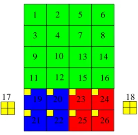
For a sub-block, we can check the coded block pattern to decide whether the CAVLC flow can be skipped. However, there are many zero coefficients that cannot be skipped by the coded block pattern. For example, Fig. 20 represents a group of four LUMA sub-blocks, where only subblock_0 comprises one nonzero coefficient and another three sub-blocks are all-zero. As mentioned in section 2.2.3, all sub-blocks must go through the CAVLC flow such that many cycle counts are wasted on zeros.

subblock_0 subblock_1

subblock_2 subblock_3

x

Fig. 20 A group of four LUMA sub-blocks

In the section, we represent statistics to show that abundant zeros cannot be skipped by the coded block pattern. To obtain the statistics, we ran several simulations using the

(39)

H.264/AVC reference software [9]. The test sequences include the following (motion from low to high): akiyo, coastguard, foreman, mobile_calendar, and Stefan. TABLE 6 shows the simulation setting. Two types of statistics are obtained and described below.

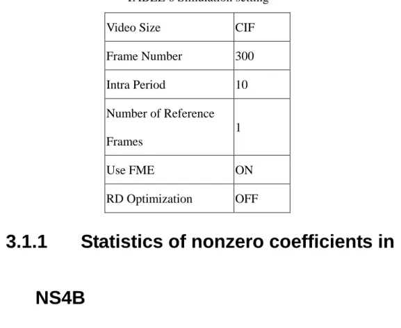
TABLE 6 Simulation setting

Video Size CIF

Frame Number 300 Intra Period 10 Number of Reference Frames 1 Use FME ON RD Optimization OFF

3.1.1 Statistics of nonzero coefficients in

NS4B

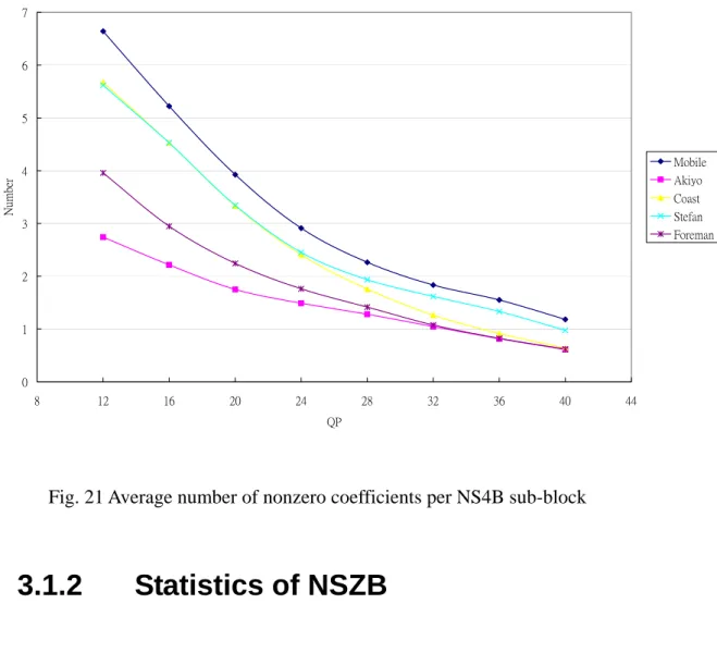
NS4B (Not Skipped 4x4 Block) denotes a sub-block, excluding CHROMA_DC, which cannot be skipped by the coded block pattern. Fig. 21 represents the average number of nonzero coefficients in a NS4B. CHROMA_DC is excluded because maximal TotalCoeff of CHROMA_DC is only four such that the average is reduced unfairly. Note that Mobile_calendar with QP equal to 12 has the highest bit-rate. Even for the highest bit-rate, a NS4B comprises less than seven nonzero coefficients; in other words, up to 60% of coefficients are zero.

(40)

0 1 2 3 4 5 6 7 8 12 16 20 24 28 32 36 40 44 QP Num ber Mobile Akiyo Coast Stefan Foreman

Fig. 21 Average number of nonzero coefficients per NS4B sub-block

3.1.2 Statistics of NSZB

NSZB (Not Skipped Zero Block) denotes an all-zero sub-block, which cannot be skipped by the coded block pattern. For example, subblock_1 of Fig. 20 can be classified as a NSZB. Fig. 22 shows how many percent of all-zero sub-blocks are NSZB. Note that a higher bit-rate results in a higher percentage. This is because a lower bit-rate induces more zero CBP bits such that more all-zero sub-blocks are covered by the CBP. Note that the percentage is significant at middle QP and low QP. Therefore, Fig. 22 proves that many all-zero sub-blocks cannot be skipped by the coded block pattern in most cases.

(41)

0.00% 10.00% 20.00% 30.00% 40.00% 50.00% 60.00% 70.00% 80.00% 8 12 16 20 24 28 32 36 40 44 QP Per cent age Akiyo Coast Stefan Foreman Mobile

Fig. 22 Percentage of NSZB in all-zero sub-blocks

3.1.3 Summary

In this section, we show the statistics to prove that abundant zero coefficients cannot be skipped by the coded block pattern. Thus CBP Look-Ahead is an inefficient method to skip zeros. To solve the problem, we propose two methods such that more zeros can be ignored. First, we use Nonzero Index Table to skip zeros in a non-all-zero sub-block. Second, we use Zero-block Codeword Table to directly encode a NSZB without going through the whole course of CAVLC flow. The two methods will be examined in section 3.4

(42)

3.2 System consideration of CAVLC

in H.264/AVC encoder

Fig. 23 shows the partial system architecture of an H.264/AVC encoder. The encoder adopts a macro-block pipeline schedule. Global Control Unit administers the progress of macro-blocks in the pipeline, where each stage comprises and processes one macro-block. Global Control Unit generates the following two things which are propagated through the pipeline registers:

1. Syntax elements which are so-called header information such as mb_type [1]. 2. Information about the macro-block at PR0 (Pipeline Register 0) such as coordinates.

P R

0 _Prediction Engine

Global Control Unit

quantized transform coefficients CBP Generator Residual Buffer P R 1 M U X 0 UVLC Entropy SRAM Interface Exp-Golomb Coding Unit CAVLC Encoder M U X 1 Bit-stream Packer H.264/AVC bit-stream Bus Interface External Memory

(43)

Prediction Engine uses data in PR0 to execute Inter or Intra prediction algorithms such that the best prediction signal can be worked out. Then Prediction Engine subtracts the prediction signal from the macro-block to obtain residual data. Finally, Prediction Engine applies transform and quantization on the residual data to obtain quantized transform coefficients. CBP Generator examines whether some coefficients are zero to determine the coded block pattern which will be stored into PR1. Moreover, the coefficients are stored into Residual Buffer. After all stages are finished, Global Control Unit grants the progress of the pipeline such that the data in PR0 goes into PR1.

Header information in PR1 is encoded in predefined order which Global Control Unit maintain by MUX 0 (Multiplexer 0) and MUX 1 (Multiplexer 1). The codeword of header information is generated by Exp-Golomb Coding Unit and is concatenated by Bit-stream Packer such that H.264/AVC bit-stream is formed. The bit-stream is written into External Memory via Bus Interface.

After encoding of header information is finished, Entropy SRAM Interface fetches coefficients of one sub-block from Residual Buffer to CAVLC Encoder. The codeword of each syntax element such as Coeff_token is sent to Bit-stream Packer via MUX 1. When encoding of the sub-block is finished, CAVLC Encoder will request Entropy SRAM Interface to fetch the next sub-block.

3.2.1 Residual

Buffer

Residual Buffer comprises five parts. The first part is Luma SRAM, which is implemented as an SRAM. Luma SRAM stores the Y component of one macro-block and Fig. 24 shows the organization of Luma SRAM.

(44)

word 0 word 1 … … word 14 word 15 Luma SRAM

Fig. 24 Organization of Luma SRAM

As mentioned in section 2.1, a macro-block comprises sixteen Y sub-blocks and one word stores one sub-block in Luma SRAM. Fig. 25 represents the mapping relation between the sub-blocks and the words.

0 1 4 5 2 3 6 7 8 9 12 13 10 11 14 15

Fig. 25 Y sub-blocks of a macro-block

Fig. 26 shows the organization of a word in Luma SRAM, where we use 14 bits to represent a coefficient. Fig. 27 shows the mapping relation between the numerical labels and the coefficients of a LUMA sub-block.

0 1 …… 14 15

14 bits

M SB LSB

(45)

0 4 8 12 1 5 9 13 2 6 10 14 3 7 11 15

Fig. 27 The coefficients of a LUMA sub-block

Fig. 28 shows the mapping relation between the numerical labels of Fig. 26 and the coefficients of a LUMA_AC sub-block. As for LUM_AC, the position “0” in Fig. 26 is useless because the DC is separated. In brief, Luma SRAM comprises 16x16x14 bits.

4 8 12 1 5 9 13 2 6 10 14 3 7 11 15

X

Fig. 28 The coefficients of a LUMA_AC sub-block

The second part is Chroma SRAM, which is implemented as an SRAM and is used to store CHROMA_AC sub-blocks. Fig. 29 shows the organization of Chroma SRAM.

word 0 word 1 … … word 6 word 7 Chroma SRAM

(46)

A macro-block comprises eight CHROMA_AC sub-blocks and one word stores one sub-block in Chroma SRAM, so there are totally eight words in Chroma SRAM. Fig. 30 shows the mapping relation between the words of Chroma SRAM and the CHROMA_AC sub-blocks of a macro-block.

0 1 4 5

2 3 6 7

U V

Fig. 30 U and V sub-blocks of a macro-block

Fig. 31 shows the organization of one word in Chroma SRAM, where we use 12 bits to represent one coefficient. Fig. 32 shows the mapping relation between the numerical labels of Fig. 31 and the coefficients of a CHROMA_AC sub-block. Because the DC is separated, the position “0” in Fig. 31 is always useless; however, it exists for the regularity of hardware architecture. In brief, Chroma SRAM comprises 8x16x12 bits.

0 1 …… 14 15

12 bits

M SB LSB

(47)

4 8 12 1 5 9 13 2 6 10 14 3 7 11 15

X

Fig. 32 Coefficients of a CHROMA_AC sub-block

The third part is LDC (Luma DC) Register, which is implemented as a register and is used to store one LUMA_DC sub-block. Fig. 33 shows the organization of LDC Register, where we use 14 bits to represent one coefficient. Fig. 34 shows the mapping relation between the numerical labels of Fig. 33 and the coefficients of a LUMA_DC sub-block. In brief, LDC Register comprises 1x16x14 bits because there are at most one LUMA_DC sub-block in one macro-block.

0 1 …… 14 15

14 bits

M SB LSB

Fig. 33 Organization of LDC Register

0 4 8 12 1 5 9 13 2 6 10 14 3 7 11 15

Fig. 34 Coefficients of a LUMA_DC sub-block

(48)

and is used to store one CHROMA_DC sub-block of U component. Fig. 35 shows the organization of CDCU Register, where we use 14 bits to store one coefficient. Fig. 36 shows the mapping relation between the numerical labels of Fig. 35 and the coefficients of a CHROMA_DC sub-block. In brief, CDCU Register comprises 1x4x14 bits because U component consists of only one CHROMA_DC sub-block.

0 1 2 3

14 bits

M SB LSB

Fig. 35 Organization of CDCU Register

0 2 1 3

Fig. 36 Coefficients of a CHROMA_DC sub-block

The final part is CDCV (Chroma DC V) Register, which is implemented as a register and is used to store one CHROMA_DC sub-block of V component. The organization of CDCV Register is the same as CDCU Register. The permutation of the coefficients in CDCV Resister is the same as Fig. 36 shows. In brief, CDCV Register comprises 1x4x14 bits because V component consists of only one CHROMA_DC sub-block.

Last but not least, as for Luma SRAM one word comprises 224 bits such that the bus seems a little wider. This is because we can write one sub-block per cycle to reduce cycle counts on macro-block level and to improve the throughput of the macro-block pipeline schedule. On the contrary, if a narrower bus is adopted, we must spend more cycle counts on

(49)

writing one macro-block into Residual Buffer than a wider bus.

3.2.2 CBP

Generator

Fig. 37 shows the architecture of CBP Generator. Prediction Engine writes one sub-block into Residual Buffer per cycle. Global Control Unit provides Global Counter for Prediction Engine to determine which sub-block is written now. In CBP Generator, we use Global Counter to generate Sub-block Index which represents one of the twenty-six sub-block as Fig. 38 shows. Global Counter Sub-block Index Comparator luma_cof chroma_cof Comparator u_dc Comparator v_dc Comparator M U X M U X 0 1 … … 24 25 … …

Nonzero Block Tag

Coded Block Pattern coded block pattern

(50)

0

1

4

5

2

3

6

7

18

19

20

21

22

23

24

25

8

9

12

13

10

11

14

15

16

17

Fig. 38 Sub-block Index of each sub-blocks in a macro-block

Prediction Engine uses luma_cof to send coefficients to Luma SRAM, uses chroma_cof to send coefficients to Chroma SRAM, uses u_dc to send coefficients to CDCU Register, and uses v_dc to send coefficients to CDCV Register. For example, when Sub-block Index is equal to three, luma_cof now comprises coefficients of sub-block “3” in Fig. 38. We use comparator to examine whether it is an all-zero sub-block. If the sub-block is all-zero, we set zero to the 3rd bit in Nonzero Block Tag, which is a 26-bit register. After the 26 sub-blocks are examined through, Nonzero Block Tag is settled and Coded Block Pattern of Fig. 37, a combinational circuit, can generate the coded block pattern for the macro-block.

3.2.3 Entropy SRAM Interface

Fig. 39 shows the architecture of Entropy SRAM Interface. Global Control Unit defines a serial number, syntax_idx_cur, for each syntax element. When syntax_idx_cur is equal to some value, it means encoding of coefficients is started and esi_enable is activated to enable Entropy SRAM Interface.

(51)

BlkIdx_cur Residual Buffer Controller fetch_step_cur sram_Chro_data reg _LumaDC reg_ChroDCU reg_ChroDCV Sub-block Type sram_Luma_data esi_enable syntax_idx_cur q_cof

Fig. 39 Architecture of Entropy SRAM Interface

“fetch_step_cur” is initialized as zero and BlkIdx_cur is initialized as zero or one depending on the macro-block type. If the macro-block is an Intra_16x16, BlkIdx_cur is initialized as zero; otherwise, BlkIdx_cur is initialized as one. BlkIdx_cur represents which sub-block Entropy SRAM Interface fetches right now. Fig. 40 shows the mapping relation between BlkIdx_cur and the sub-blocks of an Intra_16x16 macro-block. Fig. 41 shows the mapping relation between BlkIdx_cur and the sub-blocks of a non-Intra_16x16 macro-block.

(52)

1 2 5 6 3 4 7 8 9 10 13 14 11 12 15 16 19 20 21 22 23 24 25 26 17 18 0

Fig. 40 BlkIdx_cur for each sub-block of an Intra_16x16 macro-block

1 2 5 6 3 4 7 8 9 10 13 14 11 12 15 16 19 20 21 22 23 24 25 26 17 18

Fig. 41 BlkIdx_cur for each sub-block of a non-Intra_16x16 macro-block

“fetch_step_cur” represents the steps during the interaction between Entropy SRAM Interface and Residual Buffer. Fig. 42 shows the timing schedule of fetch_step_cur.

(53)

esi_enable

ADDR DATA REG

BlkIdx_cur (0)

fetch_step_cur 0 1 2 3

Fig. 42 Timing schedule of fetch_step_cur

When fetch_step_cur is equal to one, Residual Buffer Controller sends read address to Residual Buffer according to BlkIdx_cur. Then, when fetch_step_cur is equal to two, the read data is ready at the output of Residual Buffer. The output of Residual Buffer refers to sram_Luma_data, sram_Chroma_data, reg_LumaDC, reg_ChroDCU, and reg_ChroDCV in Fig. 39. “q_cof” selects one of the five output signals according to BlkIdx_cur. Finally, when fetch_step_cur is equal to three, the coefficients of the sub-block are stored into CAVLC Encoder. Moreover, Sub-block Type calculates the type of sub-block according to the current BlkIdx_cur.

3.2.4 Exp-Golomb

Coding

Unit

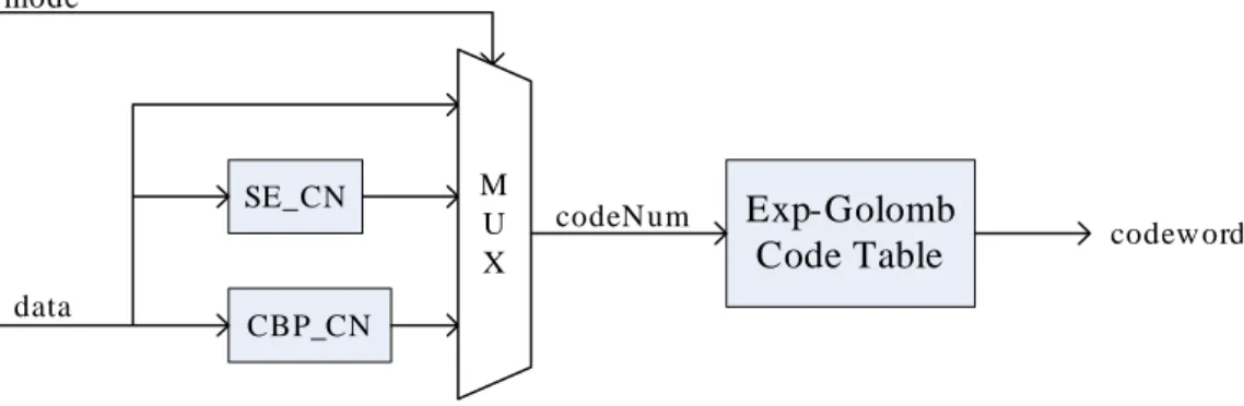
Fig. 43 shows the architecture of Exp-Golomb Coding Unit. “data” is the syntax elements from PR1 (see Fig. 23). As for Exp-Golomb Coding Unit, the syntax elements are divided into three categories as follows: UE (Unsigned Exp-Golomb), SE (Signed Exp-Golomb), and CBP [1]. Global Control Unit sends “mode” to indicate which category according to the current syntax element. We must calculate codeNum [1] of the current syntax

(54)

SE_CN CBP_CN Exp-Golomb Code Table M U X data mode codew ord codeN um

Fig. 43 Architecture of Exp-Golomb Coding Unit

As for UE, the syntax element is equal to codeNum such that “data” can be directly sent to Exp-Golomb Code Table via MUX. As for SE and CBP, we use SE_CN and CBP_CN to calculate the codeNumb respectively.

TABLE 7 shows the structure of Exp-Golomb Code Table.

TABLE 7 Structure of Exp-Golomb Code Table [1]

Codeword Range of codeNum

1 0 0 1 x0 1-2 0 0 1 x1 x0 3-6 0 0 0 1 x2 x1 x0 7-14 0 0 0 0 1 x3 x2 x1 x0 15-30 0 0 0 0 0 1 x4 x3 x2 x1 x0 31-62 … …

Fig. 44 shows the structure of codeword in TABLE 7. “M” represents the number of prefix zero bits and INFO is the value of suffix bits [11]. “codeNum” is expressed as Eq. 5 shows.

(55)

0 0 0 1 x2 x1 x0

M INFO

Fig. 44 Structure of Exp-Golomb codeword

INFO codeNum=2M −1+

Eq. 5

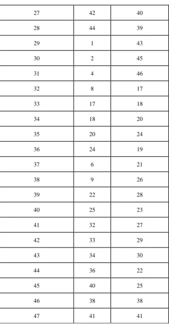
TABLE 8 shows Exp-Golomb Code Table in explicit form. SE_CN and CBP_CN are implementations of TABLE 9 and TABLE 10 respectively. As for TABLE 10, note that the mapping is different between Intra and Inter.

TABLE 8 Exp-Golomb Code Table in explicit form [1]

Bit string codeNum

1 0 0 1 0 1 0 1 1 2 0 0 1 0 0 3 0 0 1 0 1 4 0 0 1 1 0 5 0 0 1 1 1 6 0 0 0 1 0 0 0 7 0 0 0 1 0 0 1 8 0 0 0 1 0 1 0 9 … …

TABLE 9 Assignment of syntax element to codeNum for signed Exp-Golomb [1]

codeNum syntax element value

0 0 1 1 2 –1 3 2 4 –2

(56)

5 3 6 –3 k (–1)k+1 Ceil( k÷2 )

TABLE 10 Assignment of codeNum to values of CBP [1]

codeNum CBP Intra Inter 0 47 0 1 31 16 2 15 1 3 0 2 4 23 4 5 27 8 6 29 32 7 30 3 8 7 5 9 11 10 10 13 12 11 14 15 12 39 47 13 43 7 14 45 11 15 46 13 16 16 14 17 3 6 18 5 9 19 10 31 20 12 35 21 19 37 22 21 42 23 26 44 24 28 33 25 35 34 26 37 36

(57)

27 42 40 28 44 39 29 1 43 30 2 45 31 4 46 32 8 17 33 17 18 34 18 20 35 20 24 36 24 19 37 6 21 38 9 26 39 22 28 40 25 23 41 32 27 42 33 29 43 34 30 44 36 22 45 40 25 46 38 38 47 41 41

3.2.5 Bit-stream

Packer

Fig. 45 shows the input and output ports of Bit-stream Packer. Fig. 46 shows the architecture of Bit-stream Packer.

(58)

mux_word

mux_length Bit-stream Packer mux_valid

bitstream _cur bitstream _valid_cur

Fig. 45 Input and Output ports of Bit-stream Packer

residual_length_cur mux_length longer_than_31 residual_word_cur mux_word left_shifter residual_word_cur mux_word right_shifter residual_word_cur TwoByteBuf_cur mux_valid mux_valid bitstream_cur bitstream_valid_cur longer_than_31 longer_than_31

Fig. 46 Architecture of Bit-stream Packer

“mux_word”, “mux_length”, and “mux_valid” are output signals of MUX 1 (See Fig. 23). “mux_word” carries the codeword of some syntax element and mux_length represents the length of the codeword. Fig. 47 shows the structure of mux_word, where the codeword is “00101” and mux_length is equal to five. Note that mux_word is left-alignment.

(59)

0 0 1 0 1 0 0 …… 0 “00101＂

mux_word

32 bits

Fig. 47 Structure of mux_word

When mux_valid is high, it means that mux_word is valid and that we must concatenate mux_word into residual_word_cur, a 32-bit register. The length of the codeword in residual_word_cur is represented by residual_length_cur. Fig. 48 shows the structure of residual_word_cur, where the codeword is “00101” and residual_length_cur is equal to five. Note that residual_word_cur is right-alignment.

0 0 1 0 1 0 0 …… 0

“00101＂ residual_word_cur

32 bits

Fig. 48 Structure of residual_word_cur

When mux_valid is high, if the sum of mux_length and residual_length_cur is smaller than 32 (longer_than_31 is low), residual_word_cur is updated by left_shifter as Fig. 49 shows.

(60)

32 bits mux_word 32 bits residual_word_cur left_shifter 32 bits 32 bits 32 bits residual_word_cur update...

Fig. 49 Updating of residual_word_cur by left_shifter when longer_than_31 is low

“left_shifter” is a right-alignment signal of 64 bits and consists of the concatenation of residual_word_cur and mux_word. On the other hand, if the sum of residual_length_cur and mux_length is larger than 31 (longer_than_31 is high), bitstream_cur is updated as shown in Fig. 50 and bitstream_valid_cur is high such that Bus Interface (see Fig. 23) can fetch the updated bitstream_cur.

(61)

32 bits mux_word 32 bits residual_word_cur right_shifter 32 bits 32 bits 32 bits bitstream_cur update... A B C A B

Fig. 50 Updating of bitstream_cur by right_shifter

“bitstream_cur” is a register of 32 bits; in other words, we send 32 bits of bit-stream to Bus Interface in one cycle. “right_shifter” is a left-alignment signal of 64 bits and consists of the concatenation of residual_word_cur and mux_word. The remaining part, “C”, is stored into residual_word_cur.

Moreover, TwoByteBuf_cur is a register of 16 bits and comprises the last two bytes of H.264/AVC bit-stream stored in External Memory (see Fig. 23). We use TwoByteBuf_cur and right_shiter to determine whether emulation prevention byte [1], a byte equal to 0x03, is necessary to be inserted into bitstream_cur. The main purpose of emulation prevention bytes is to ensure that start code prefix [1], a sequence of three bytes equal to 0x000001, occurs only at the beginning of the H.264/AVC bit-stream. When the following successive three bytes are found in the raw byte sequence, emulation prevention byte is inserted:

(62)

2. 0x000001 Æ 0x00000301 3. 0x000002 Æ 0x00000302 4. 0x000003 Æ 0x00000303

The usage of TwoByteBuf_cur is illustrated in Fig. 51. “right_shifter[63:32]” is divided into four bytes and the arrowhead is the insert position of emulation prevention byte. There are only seven cases according to the analysis [12]. For example, case 1 is illustrated in Fig. 52, where the number is hexadecimal. After insertion, bitstream_cur becomes 0x03000003 and 0x0002 is stored into residual_word_cur.

right_shifter[63:32] TwoByteBuf_cur case 0 case 1 case 2 case 3 case 4 case 5 case 6

(63)

00 00 00 00 00 02

TwoByteBuf_cur right_shifter[63:32]

Insertion...

03 00 00 03 00 02

Fig. 52 Example for case 1

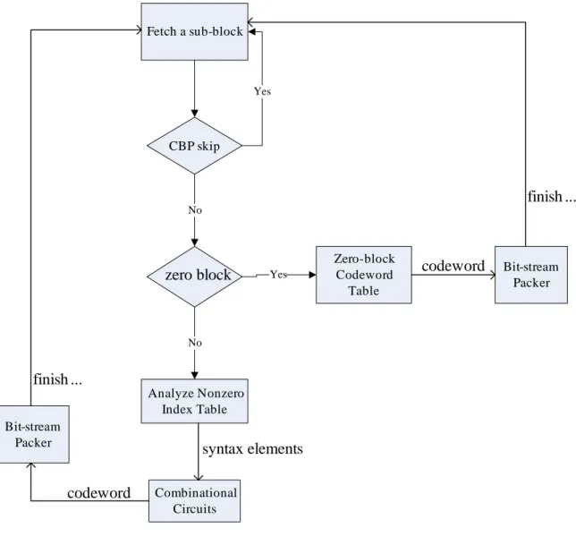
3.3 Encoding flow of proposed

CAVLC encoder

Fig. 53 represents encoding flow of the proposed CAVLC encoder. Entropy SRAM Interface provides the proposed CAVLC encoder with the coded block pattern and coefficients of a sub-block.

(64)

Fetch a sub-block CBP skip Yes No Zero-block Codeword Table Yes Analyze Nonzero Index Table No

zero block codeword Bit-stream _Packer finish ... Combinational Circuits syntax elements codeword Bit-stream Packer finish ...

Fig. 53 Encoding flow of the proposed CAVLC encoder

The proposed CAVLC encoder uses the coded block pattern to determine whether the sub-block can be skipped. If the sub-block can be skipped, there are no further steps and we fetch the next sub-block from Entropy SRAM Interface. Otherwise, if the sub-block cannot be skipped, the coefficients are loaded into Input Buffer, as Fig. 54 shows. Nonzero Index Table concurrently records which coefficients are nonzero by setting bit “1”. Both Input Buffer and Nonzero Index Table are registers constructed in the proposed CAVLC encoder.

(65)

0 0 0 0 0 0 0 0 1 0 -1 -1 1 0 3 0 Input Buffer

15 14 13 12 11 10 9 8 7 6 5 4 3 2 1 0

0 0 0 0 0 0 0 0 1 0 1 1 1 0 1 0 Nonzero Index Table

15 14 13 12 11 10 9 8 7 6 5 4 3 2 1 0

Fig. 54 Input Buffer and Nonzero Index Table

If all bits are zero in Nonzero Index Table, as Fig. 55 shows, it means that the sub-block is NSZB. Zero-block Codeword Table generates the codeword of the NSZB and Bit-stream Packer concatenates the codeword in parallel. Then the encoding flow is terminated earlier such that we save cycle counts for collecting syntax elements of the NSZB.

0 0 0 0 0 0 0 0 0 0 0 0 0 0 0 0 Input Buffer

15 14 13 12 11 10 9 8 7 6 5 4 3 2 1 0

Fig. 55 Nonzero Index Table for an all-zero sub-block

Otherwise, if Nonzero Index Table consists of nonzero bits (see Fig. 54), it means that the sub-block consists of nonzero coefficients. This thesis refers to a sub-block comprising nonzero coefficients as NAZ (Not All Zero). We analyze Nonzero Index Table to obtain syntax elements whose codeword are generated by combinational circuits and are concatenated by Bit-stream Packer. After all syntax elements of the sub-block are encoded into H.264/AVC bit-stream, the encoding of the NAZ sub-block is finished and we can fetch the next sub-block.

(66)

Nonzero Index Table makes it possible to directly encode significant coefficients such that we can save cycle counts on zero coefficients in NAZ. We can encode one nonzero coefficient every cycle by updating Nonzero Index Table. Fig. 56 and Fig. 57 show the updating. At some cycle, as shown in Fig. 56, we aim at the coefficient at index “7” and the codeword of the coefficient is concurrently generated by combinational circuits. At the next cycle (see Fig. 57), Nonzero Index Table is updated and we aim at the coefficient at index “4” such that the zeros between index “4” and “7” are ignored. Hence, Nonzero Index Table saves cycle counts on zero coefficients in NAZ.

0 0 0 0 0 0 0 0 1 0 0 -1 1 0 3 0 Input Buffer

15 14 13 12 11 10 9 8 7 6 5 4 3 2 1 0

Fig. 56 Coefficient at index 7 is being encoded

0 0 0 0 0 0 0 0 1 0 0 -1 1 0 3 0 Input Buffer

15 14 13 12 11 10 9 8 7 6 5 4 3 2 1 0

(67)

3.4 Architecture of proposed CAVLC

encoder

According to section 3.3, sub-blocks can be divided into three categories in terms of encoding flow:

1. NAZ: as mentioned in section 3.3. 2. NSZB: as mentioned in section 3.1.2.

3. CS (CBP Skip): a sub-block which can be skipped by the coded block pattern.

In this section, we first describe the architecture of the proposed CAVLC encoder. Then, in the following three sections, we cycle-wise explain the hardware operation for NAZ, NSZB, and CS to manifest the advantages of our design.

Fig. 58 shows the architecture of the proposed CAVLC encoder. “cavlc_data_ready” fetches sixteen coefficients in one cycle. If the sub-block comprises less than sixteen coefficients like CHROMA_DC, Entropy SRAM Interface automatically appends zeros. According to the sub-block type and the coded block pattern, we determine whether the sub-block is CS.

(68)

cavlc_data _ready cavlc_scan cavlc_coding cavlc_coding_level cavlc_coding_crun cavlc_mux cavlc_nunl sram_nonzero Entropy SRAM Interface Bit-stream Packer Nonzero Index Table Zero-block Codeword Table

Fig. 58 Architecture of the proposed CAVLC encoder

As for a sub-block of NSZB or NAZ, the sixteen coefficients including the appending zeros are stored into Input Buffer, which comprises sixteen 16-bit registers, as Fig. 59 shows. Input Buffer is constructed in cavlc_data_ready. The coefficients are put into Input Buffer in zigzag scan order. We consider Input Buffer as a 1-D array and index “0” represents the DC. The greater the index is, the higher the frequency is. Nonzero Index Table comprises sixteen 1-bit registers and indicates which coefficients are nonzero. When the coefficients are stored, we concurrently check which coefficients are zeros. If a coefficient is nonzero, we set one to the corresponding bit in Nonzero Index Table. The index of Nonzero Index Table is the same as Input Buffer.

低成本高效率內容適應性可變長度編碼器之設計

國立交通大學

電子工程學系 電子研究所碩士班

碩 士 論 文

低成本高效率內容適應性可變長度編碼器之設計

A Low Cost and High Throughput CAVLC Encoder

Design

學生 :吳 秈 璟

指導教授 :張添烜 博士

低成本高效率內容適應性可變長度編碼器之設計

A Low Cost and High Throughput CAVLC Encoder

Design

研 究 生 : 吳秈璟 Student

:

Sian-Jing

Wu

指導教授 : 張添烜 博士 Advisor

:

Dr.

Tian-Sheuan

Chang

國 立 交 通 大 學

電子工程學系 電子研究所 碩士班

碩 士 論 文

低成本高效率內容適應性可變長度編碼器之設計

學生 : 吳秈璟

指導教授 : 張添烜 博士

國立交通大學

電子工程學系 電子研究所碩士班

摘要

A Low Cost and High Throughput CAVLC Encoder

Design

Student : Sian-Jing Wu

Advisor : Dr. Tian-Sheuan Chang

Institute of Electronics

National Chiao Tung University

ABSTRACT

誌 謝

Contents

List of Figures

List of Tables

Chapter 1. Introduction

1.1 Motivation

1.2 Organization of thesis

Chapter 2. Overview of CAVLC in

H.264/AVC

2.1 Overview of an H.264/AVC

encoder

+

+

2.2 Overview of block types

2.2.1

Partitions of a macro-block

0

1

4

5

2

3

6

7

18

19

20

21

22

23

24

25

8

9

12

13

10

11

14

15

16

17

2.2.2

電子工程學系電子研究所碩士班

碩士論文

學生 :吳秈璟

指導教授 :張添烜博士

研究生 : 吳秈璟 Student

指導教授 : 張添烜博士 Advisor

國立交通大學

電子工程學系電子研究所碩士班

碩士論文

指導教授 : 張添烜博士

電子工程學系電子研究所碩士班

誌謝