Analysis of Elliptical Waveguides by Method of Fundamental Solutions

MMIC, with chip size of 1.5⫻ 1 mm. 4. MEASUREMENT

The measurement is performed by putting the VCO MMIC chip into a test fixture, as shown in Figure 4. A test board is used to supply DC power to the chip and to output the oscillating signal through the SMA connector. There are two capacitors (100 pF and 10␮F, respectively) connected in parallel to each DC supply line, which is used to bypass the undesired RF signals. The oscillating curve is displayed on an MS288C spectrum analyzer. The mea-surement results are shown in Figures 5 and 6. The operation condition for this VCO MMIC measurement is: Vd⫽ 3.0 V, Ids⫽ 18 mA. Figure 5 shows a typical oscillating signal with oscillating frequency of 25.0232 GHz, and Figure 6 shows the measured oscillating frequency and the associated output-power tuning curves. The designed VCO MMIC has a tuning range of 1.4 GHz at around 25.7 GHz with an output power of about 8 dBm.

As mentioned above, the VCO MMIC was measured by insert-ing it into the test fixture shown in Figure 4. Clearly, the measured output power will be less than that released by the chip itself, due to the loss of output microstrip and the connector in the test ficture. On-wafer measurement result shows a loss of about 3 dBm for them; so, the output power released by the chip itself should be about 11 dBm.

5. CONCLUSION

An active-biased 26-GHz VCO MMIC, based on a 0.25-␮m GaAS pHEMT process, has been presented in this paper. Its tuning range is 1.4 GHz with a central frequency of 25.7 GHz, and the output power is 11⫾ 1 dBm. The fabricated VCO MMIC chip size is 1.5⫻ 1.0 mm.

ACKNOWLEDGMENTS

This work was financially supported by the Chinese National Hi-Tech “863” Plan (2002AA135270), the Science and Technol-ogy Development Foundation of Shanghai, China (021111122), and the Research and Development Foundation on Applied Mate-rials of Shanghai, China (0204).

REFERENCES

1. A. Welthof, H. J. Siweris, et al., A 38/76-GHz automotive radar chip set fabricated by a low-cost pHEMT technology, IEEE MTT-S Int Micro-wave Symp Dig (2002), Seattle, WA 1855–1858.

2. N. Priestly, K. Newsome and I. Dale, A Gunn diode-based surface mount 77-GHz oscillator for automotive applications, IEEE MMT-S Int Microwave Symp Dig (2002), Seattle, WA 1863–1866.

3. M. Camiade, D. Domnesque et al., Full MMIC millimeter-wave front-end for a 76.5-GHz adaptive cruise-control car radar, IEEE MTT-S Int Symp Dig (1999), Anaheim, CA 1489 –1492.

4. X. Zhang et al., Comparison of the phase noise performance of

HEMT-and HBT-based oscillators, IEEE Int Symp Dig (1995), OrlHEMT-ando, FL 697– 680.

5. A. Megej and K. Beilenhoff, Active biasing technique for compact wide-band voltage controlled oscillators, IEEE MTT-S Int Symp Dig (2001), Pheonix, AZ 1419 –1422.

© 2005 Wiley Periodicals, Inc.

ANALYSIS OF ELLIPTICAL

WAVEGUIDES BY THE METHOD OF

FUNDAMENTAL SOLUTIONS

D. L. Young, S. P. Hu, C. W. Chen, C. M. Fan, and K. Murugesan

Department of Civil Engineering & Hydrotech Research Institute National Taiwan University

Taipei, Taiwan, Republic of China

Received 25 August 2004

ABSTRACT: The present work describes the application of the method of

fundamental solutions (MFS) for the solution of cutoff wavelengths of ellip-tical waveguides. Since the MFS employs a formulation using boundary values only, the cutoff wavelengths are determined by applying the singular value decomposition (SVD) technique. The use of the MFS to solve the gov-erning (Helmholtz) equation guarantees a solution without singularities, since it does not use discretized points to determine the solution at the inte-rior of the computational domain. The combination of the MFS and SVD techniques has resulted in a simpler and efficient numerical solution proce-dure, as compared to other schemes. © 2005 Wiley Periodicals, Inc.

Microwave Opt Technol Lett 44: 552–558, 2005; Published online in Wiley InterScience (www.interscience.wiley.com). DOI 10.1002/mop. 20695

Key words: method of fundamental solutions; singular value

decompo-sition; elliptical waveguides; Helmholtz equation

1. INTRODUCTION

Elliptical waveguides have been widely applied in many engineer-ing fields. Chu [1] presented the theory of the transmission of electromagnetic waves in hollow conducting pipes of elliptic cross section, and reported numerical results for the cutoff frequency and the attenuation for six waves. It is very crucial to determine the cutoff wavelengths of an elliptical waveguide for the design of waveguides; hence, this field has attracted many researchers in the recent past. Kinzer and Wilson [2] published the first approximate formulae to determine the cutoff frequency of the TE_c01, TM_c11, and TM_s11modes for a given elliptical cross section. Kretzschemar [3] obtained the curves of the cutoff wavelengths for 19 successive modes. Zhang and Shen presented analytical solutions of elliptical waveguides [4], and most of the attention was paid to computing the zeros of the modified Mathieu functions of the first kind. Recently, a numerical analysis of elliptical waveguides using the differential-quadrature method was conducted by Shu [5]. Gold-berg et al. [6] calculated the cutoff wavelengths for the six lowest modes and gave a correction to the field pattern plotted in Chu [1]. Lately, a meshless collocation method with the Wendland radial basis functions was conducted by Jiang et al. [7].

Mesh-dependent methods such as the finite-element method, finite-difference method, and finite-volume method require distrib-uted grid points at the interior of the domain for computing the field variables. Significant computational effort is required for pre-processing the mesh generation in the above methods. In particular, to find numerical solutions for irregular domains in-Figure 6 Oscillating frequency and output-power tuning curves

volves the strenuous task of mesh generation when the above numerical methods are used. For the case of waveguide problems, the numerical results have to compute the zeros of the modified Mathieu functions of the first kind. However, it is not convenient to determine the eigenmode sequence of an elliptical waveguide with given ellipticity for such computations, since a large number of calculations are required. In addition, the high-order modes in an eigenmode sequence may be missed during the computation using conventional numerical methods, since they use only a definite number of grid points.

Meshless methods have become popular in the recent decade, and many efforts have been devoted to the development of mesh-less methods by many researchers [8, 9]. In the present work, a numerical method based on the method of fundamental solutions (MFS) is devised to solve the cutoff wavelengths of elliptical waveguides. Unlike the FEM or FDM, the present method does not use any domain-discretization scheme to obtain the grid points inside the computational domain and, hence, the MFS is normally considered as a meshless numerical method. In the MFS, only the equations governing the boundary node points are solved, thus saving a lot of computational time and effort compared to other numerical schemes. The solutions at the interior domain are ob-tained only by means of a simple interpolation based on the MFS. The MFS [10, 11] has been applied successfully to deal with many types of boundary-value problems. Chen et al. [12] used the conventional BEM in conjunction with the singular value decom-position (SVD) technique to solve eigenvalue problems governed by the Helmholtz equation, and they adopted SVD technique [13] to determine the eigenvalues. In the present work, the MFS is applied to solve an elliptical-waveguide problem with an aim to determine the cutoff wavelengths for TE and TM modes. Details about the governing equations used are discussed in section 2. A discussion of the predicted results is provided in section 3. The conclusions based on the present work are discussed in section 4. 2. GOVERNING EQUATIONS AND BOUNDARY CONDITIONS The transverse magnetic (TM) and transverse electric (TE) waves are defined using the eigenfunctions of the Helmholtz equation with both Dirichlet and Neumann boundary conditions as follows:

ⵜ2_{␾ ⫹ k}

c

2_{␾ ⫽ 0, (1)}

where kcis the cutoff wavenumber. For the case of TM waves, Hz ⫽ 0 and␸ ⫽ Ez, while for the TE waves, Ez⫽ 0 and␸ ⫽ Hz. The TM waves should satisfy the following Dirichlet boundary condition:

␾兩⌫⫽ Ez兩⌫⫽ 0. (2)

The TE waves satisfy the Neumann boundary condition, given by ⭸␾

⭸n

冏

⭸n

冏

where⌫ refers the boundary of the waveguide and is written as the following equation for an ellipse:

冉

冊

冉

冊

Here, the parameters a and b are semi-major axis and semi-minor axis, respectively, and eccentricity e⫽ (公a2_{⫺ b}2_/a).

The purpose of the study is to solve the eigenvalue kcof the resultant matrix obtained from the Helmholtz equation. Once the eigenvalues are known, the cutoff wavelengths of the waveguides can be computed. The application of the MFS to solve the Helm-holtz equation for the TM and TE modes is discussed in the following sections.

3. APPLICATION OF MFS

The MFS makes use of the field variables known at the boundary to obtain the solution for the interior of the domain. From the principle of the MFS, for a given governing equation, the free-space Green’s function needs to be satisfied. In the present cases, the free-space Green’s function is written for the Helmholtz equa-tion as follows:

ⵜ2_{G共 xជ兲 ⫹ k}

c

2_{G共 xជ兲 ⫽ ⫺␦共xជ ⫺ ␰ជ兲, (5)}

where␦( x ⫺ ␰) is the Dirac delta function, xជ is the position of the field point, and␰ជ is the position of the source point. From these conditions (consider in polar coordinate),ⵜ2_{G( xជ, ␰ជ) ⫹ k}2_{G( xជ,}

␰ជ) ⫽ 0 can be obtained as expected at rជ ⫽ 0. So the following form can be solved. Eq. (5) can simply be solved by r2_{G⬙ ⫹ rG ⫹}

(k2_r2 _{⫺ 0)G ⫽ 0. The fundamental solution can be solved by}

Figure 1 Points distribution: (a) e ⫽ 0.1; (b) e ⫽ 0.9 (total point numbers are 20)

using the Bessel function, where G(ri) ⫽ (⫺i/4) H0 (2)_(k

cri) ⫽ (⫺i/4)[ J₀(kcri) ⫺ iY0(kcri)] is the fundamental solution. Using the above expression, the approximate solution for the Helmholtz equation is obtained as follows:

␾共x៝兲 ⫽i

冘

N

␣j␾G共rij兲. (6)

For the case of TE mode, the Neumann boundary condition to be used by MFS is stated as follows:

⭸␾ ⭸n 共xi៝兲 ⫽

冘

and the normal derivative is expressed by the following expres-sion: ⭸G共rij兲 ⭸ni ⫽ ⭸G共rij兲 ⭸r ⭸r ⭸ni⫽ ⫺

冋

4r kc

册

where ␣j␾ denotes the coefficients to be determined using the boundary values by the method of collocation, ␾共x៝兲 is the dis-i placement of the ith_{node, r}

ijis the distance between the ithand the jth _{nodes and is defined as r}

ij ⫽ 兩rជi ⫺ rជj兩, H0

(2) _{is the second}

Hankel function of order zero, J₀is the Bessel function of the first kind of order zero, J₁ is the Bessel function of the first kind of order one, Y₀is the Bessel function of the second kind of order

zero, Y₁is the Bessel function of the second kind of order one, and N is the number of source points.

From Eqs. (6) and (7), the approximate solution using MFS is expressed in matrix form by the following expression:

关Aij⍀兴兵␣j␾其 ⫽ 兵␾兩⌫其, (9) where the coefficient matrix [Aij⍀] contains the summation of the radial basis functions for the Helmholtz equation for the solution domain⍀.

In the case of the MFS, the first step in obtaining the approx-imate solution is the determination of the values of ␣j␾ for the solution domain using the boundary values. For the case of the cutoff wavelengths ␭c of the elliptical-waveguides problem, the Figure 2 Cutoff wavelengths␭cfor (a) TM waves, with e⫽ 0.1; (b) TM waves with e ⫽ 0.9; (c) TE waves with e ⫽ 0.1; (d) TE waves with e ⫽ 0.9

TABLE 1 Normalized Cutoff Wavelengths of TM Modes for

eⴝ 0.1 Analytical (Ref. [4]) MFS RBF (Ref. [8]) N ⫽ 20 N⫽ 25 N⫽ 49 N⫽ 171 1 2.6062 2.6062 2.6062 2.6081 2.6062 2 1.6377 1.6377 1.6377 1.6435 1.6378 3 1.6336 1.6336 1.6336 1.6393 1.6337 4 1.2204 1.2204 1.2204 1.2337 1.2205 5 1.2204 1.2204 1.2204 1.2334 1.2204 6 1.1353 1.1353 1.1353 1.1552 1.1353 7 0.9823 0.9823 0.9823 1.0197 0.9823 8 0.9823 0.9823 0.9823 1.0196 0.9823 9 0.8945 0.8945 0.8945 0.9490 0.8945

behavior for the TM and TE modes at the Dirichlet and Neumann boundary conditions are zero. In the above equation, the right-hand side is zero because of the Dirichlet and Neumann boundary conditions. But from the basic principle of the MFS, the values of ␣j␾cannot be zero; hence, in order to satisfy Eq. (9), the coefficient matrix [A] has to be singular. Using the SVD technique, the singular matrix [A] can be solved for the eigenvalues kc of the matrix. These eigenvalues kcare nothing but the characteristics of the coefficient matrix; in other words, the wavenumbers for the waveguide problem. From the plot of minimum singular values of the matrix versus kc, the local minimum of the determinant can be found as the eigenvalues using the SVD technique. After deter-mining the eigenvalues, the eigenmodes are obtained by setting a

normalized value to be one in an element for the nontrivial vector. By substituting the eigenvalues and boundary mode into Eq. (6), the interior mode can be obtained. The MFS requires mesh points only at the boundary in order to determine the values of␣j␾and the values of the field variable in the interior domain can be computed by means of interpolation using the semi-analytics solution of Eq. (6). This makes the present numerical scheme nearly a meshless procedure, which is highly efficient for handling such eigenmode problems.

4. NUMERICAL RESULTS

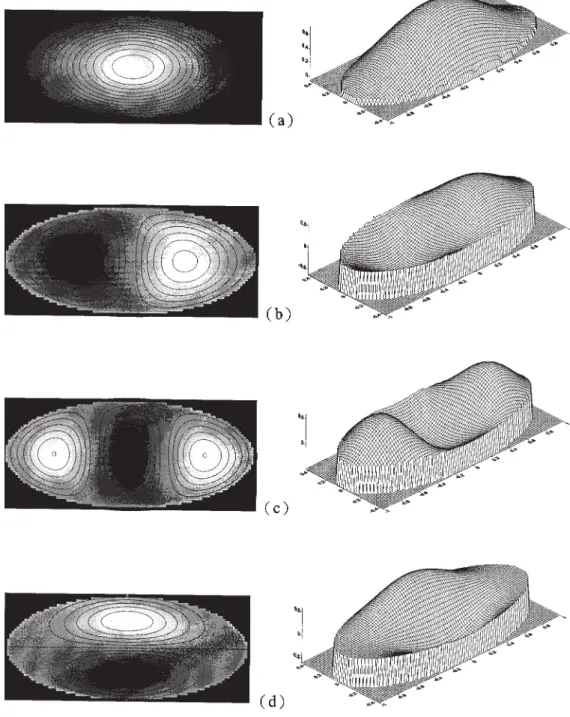
The determination of the cutoff wavelength of elliptical waveguides in TM and TE modes, as considered by Jiang et al. [7] Figure 3 Phenomena of the TM mode for e⫽ 0.1: (a) kc⫽ 2.4; (b) kc⫽ 3.8; (c) kc⫽ 5.1; (d) kc⫽ 6.4

and the analytical solutions [4], is taken as a test problem in the present work. Initially, the application of the MFS to solve the Helmholtz equation results in a singular matrix, as given by Eq. (9). The eigenvalues are first obtained by solving the singular matrix using the SVD technique. The points distribution is shown in Figure 1. And Figures 2(a)–2(d) show the plots of singular values versus the (2␲/kc). The minimum values of the above plots in the x-axis gives the required cutoff wavelengths, which are characteristic of the singular matrix.

4.1 Cutoff Wavelengths of TM Mode for e⫽ 0.1

The cutoff wavelengths for the TM mode with e⫽ 0.1 are solved by using the SVD technique, and these results are tabulated along with the results of Jiang et al., as shown in Table 1. The phenom-ena of vibrating eigenmodes of TM mode are shown in Figure 3. In order to improve the accuracy of the prediction, Jiang et al. used two different meshes having N⫽ 49 points and N ⫽ 171 points for both the TM and TE modes for eccentricity values equal to 0.1 and 0.9, respectively. Since the MFS solves only the number of equations equal to the number of boundary points of the solution domain, our method could produce the results as that of Jiang et al. obtained with a greater number of mesh points, as seen from Table 1. We also increased the number of boundary points in order to improve the accuracy of our predictions. The results obtained with N⫽ 25 give almost the same results as that of N ⫽ 20, but at the same time agreed closely with the analytical results [4]. One can easily infer that our results are even better than the results of Jiang et al. [8], which were obtained with N ⫽ 49. Also, they can achieve the less accurate results by using the node point N⫽ 171, whereas we have closely achieved almost indentical solutions to the analytical results in [4], even with N⫽ 25.

4.2 Cutoff Wavelengths of TE Mode for e⫽ 0.1

Using the SVD technique, the cutoff wavelengths for the TE mode are obtained for e ⫽ 0.1. Table 2 shows the comparison of the present results with those of Jiang et al. For the lower values of eccentricity, the MFS results obtained using N⫽ 20 and N ⫽ 25 do not show much difference, as observed in the table. At the same time, the present results are in close agreement with the analytical results [4]. But the RBF method [7] could not produce results closer to the analytical solutions even using a finer mesh of N⫽ 171. One can easily observe that the difference between the RBF results and the analytical results has increased with finer grid points, as observed in the last column of Table 3. This is another proof that the MFS can predict results of the cutoff wavelengths more accurate than other numerical methods.

4.3 Cutoff Wavelengths of TM Mode for e⫽ 0.9

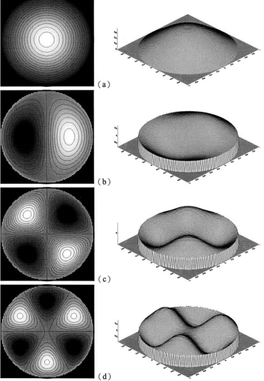
The results for the cutoff wavelengths are also obtained for e ⫽ 0.9 using N⫽ 20 and 25 for the MFS method. A comparison of our results with those of Jiang et al. [8] for two different meshes is shown in Table 3. The vibrating eigenmodes phenomenon of TM mode is described in Figure 4. Although results closer to the analytical solutions [4] were achieved using only N⫽ 20 for the case of e ⫽ 0.1, a slightly finer mesh (N ⫽ 25) is required for obtaining results closer to the analytical solution for the case of e⫽ 0.9. But again the number of points used in the MFS method is much less compared to the number of points used by Jiang et al. [7]. It can be observed from Table 3 that even with N⫽ 171, the method used by the above authors could not predict the cutoff wavelengths closer to the analytical solution [4]. This proves that the MFS is capable of predicting the TM-mode cutoff wavelengths more accurately than other numerical methods and also that it requires a lower number of grid points to achieve results closer to the analytical solutions [4].

4.4 Cutoff Wavelengths of TE Mode for e⫽ 0.9

The cutoff wavelengths for the case of the TE mode with e⫽ 0.9 are obtained by using the MFS method. These results are shown in Table 4 along with the results of Jiang et al. [7] for different values of grid points. The tabulated results indicate that the present results obtained using N⫽ 25 are almost the same as that of the analytical solution [4]. Even with N⫽ 20, our results are very close to the analytical results. However, the results obtained using RBF method [7] with N ⫽ 171 are quite far from the analytical solutions. We have observed from the above results that the MFS can predict the cutoff wavelengths accurately almost indepen-dently of the mesh sizes, whether N⫽ 20 or N ⫽ 25 for small as well as larger values of eccentricity, but the RBF method is found to be very sensitive for the value of eccentricity.

5. CONCLUSION

The 2D homogeneous Helmholtz equation governing the cutoff wavelengths of elliptical waveguides behavior has been solved using the MFS along with the SVD technique. The ability of the MFS to compute the eigenvalues and eigenmodes of TM and TE modes for an elliptical waveguide has been tested successfully. The cutoff wavelengths calculated for the TM and TE modes of the elliptical waveguide with e ⫽ 0.1 and 0.9 show very good agreement with the analytical results. A significant saving in computational effort and time can be achieved by using the MFS to solve the Helmholtz equation, since the MFS does not require the interior grid points. The MFS can predict the cutoff wave-lengths more accurately, even with a coarse mesh, as compared to those of the RBF method obtained with a relatively finer mesh.

TABLE 3 Normalized Cutoff Wavelengths of TM Waves for

eⴝ 0.9 Analytical (Ref. [4]) MFS RBF (Ref. [8]) N ⫽ 20 N⫽ 25 N⫽ 49 N⫽ 171 1 1.4906 1.4908 1.4906 1.4915 1.4906 2 1.1607 1.1607 1.1607 1.1693 1.1609 3 0.9375 0.9375 0.9375 0.9403 0.9382 4 0.8093 0.8093 0.8093 0.8449 0.8093 5 0.7803 0.7799 0.7803 0.8099 0.7781 6 0.7083 0.7071 0.7083 0.7070 0.7084 7 0.6651 0.6642 0.6651 0.7052 0.6643 8 0.6262 0.6260 0.6262 0.6686 0.6248 9 0.5780 0.5761 0.5780 0.6402 0.5748

TABLE 2 Normalized Cutoff Wavelengths of TE Modes for

eⴝ 0.1 Analytical (Ref. [4]) MFS RBF (Ref. [8]) N ⫽ 20 N⫽ 25 N⫽ 49 N⫽ 171 1 3.4119 3.4119 3.4119 3.3854 3.4039 2 3.3962 3.3962 3.3962 3.3700 3.3936 3 2.0521 2.0521 2.0521 2.0479 2.0516 4 2.0520 2.0520 2.0520 2.0749 2.0515 5 1.6356 1.6356 1.6356 1.6482 1.6372 6 1.4918 1.4918 1.4918 1.5409 1.4943 7 1.4918 1.4918 1.4918 1.5408 1.4943 8 1.1786 1.1786 1.1786 1.2003 1.8687 9 1.1786 1.1786 1.1786 1.2003 1.8687

Also, the stability of the MFS is highly reliable with varying values of eccentricity in the computation of cutoff wavelengths. This demonstrates that the MFS is a potential meshless numerical scheme for solving eigenvalue problems.

REFERENCES

1. L.J. Chu, Electromagnetics in elliptic hollow pipes of metal, J Appl Phys 9 (1938), 583–591.

2. J.P. Kinzer and I.G. Wilson, Some results on cylindrical cavity reso-nators, Bell Syst Tech J (1947), 423– 431.

3. J.G. Kretzschmar, Wave propagation in the hollow conducting ellip-tical waveguide, IEEE Trans Microwave Theory Tech MTT 18 (1970), 547–554.

4. S.J. Zhang and Y.C. Shen, Eigenmode sequence for an elliptical waveguides with arbitrary ellipticity, IEEE Trans Microwave Theory Tech 45 (1995), 1603–1608.

Figure 4 Phenomena of the TM mode for e⫽ 0.9: (a) kc⫽ 4.2; (b) kc⫽ 5.4; (c) kc⫽ 6.7; (d) kc⫽ 7.7

TABLE 4 Normalized Cutoff Wavelengths of TE Waves for

eⴝ 0.9 Analytical (Ref. [4]) MFS RBF (Ref. [8]) N ⫽ 20 N⫽ 25 N⫽ 49 N⫽ 171 1 3.3482 3.3481 3.3482 3.3415 3.3475 2 1.8287 1.8287 1.8287 1.8508 1.8291 3 1.5650 1.5649 1.5650 1.5695 1.5652 4 1.2654 1.2654 1.2654 1.3917 1.2769 5 1.2292 1.2292 1.2292 1.2557 1.2292 6 0.9986 0.9986 0.9986 1.0889 1.0063 7 0.9698 0.9698 0.9698 0.9135 0.9969 8 0.8340 0.8340 0.8340 0.8376 0.8535 9 0.8177 0.8175 0.8177 0.8013 0.8188

5. C. Shu, Analysis of elliptical waveguides by differential quadrature method, IEEE Trans Microwave Theory Tech 48 (2000), 319 –322. 6. D.A. Goldberg, L.J. Laslett, and R.A. Rimmer, Modes of elliptical

waveguides: A correction, IEEE Trans Microwave Theory Tech 38 (1990), 1603–1608.

7. P.L. Jiang, S.Q. Li, and C.H. Chan, Analysis of elliptical waveguides by a meshless collocation method with the wendland radial basis functions, Microwave Opt Technol Lett 32 (2002), 162–165. 8. A. Karageorghis, The method of fundamental solutions for the

calcu-lation of the eigenvalues of the Helmholtz equation, Appl Mathem Lett 14 (2001), 837– 842.

9. C.C. Tsai, D.L. Young, and A.-D. Cheng, Meshless BEM for steady three-dimensional Stokes Flows, Proc Int Conf Computat Engg Sci-ences, 2001.

10. M.A. Golberg, C.S. Chen, H. Bowman, and H. Power, Some com-ments on the use of radial basis functions in the dual reciprocity method, Computat Mechan 21 (1998), 141–148.

11. Y.S. Smyrlis and A. Karageorghis, Some aspects of the method of fundamental solutions for certain harmonic problems, J Scientific Computing 16 (2001), 341–371.

12. J.T. Chen, S.R. Lin, K.H. Chen, I.L. Chen, and S.W. Chyuan, Eigen-nalysis for membranes with stringers using conventional BEM in conjunction with SVD technique, Comput Methods Appl Mechan Engg 192 (2003), 1299 –1322.

13. W.H. Press et al., Numerical recipes in Fortran 77: The art of scientific computing, Cambridge University Press, Cambridge, UK, 1999.

© 2005 Wiley Periodicals, Inc.

THE PMD EFFECT IN OSNR

MONITORING

F. G. Sun, Z. G. Lu, G. Z. Xiao, and C. P. Grover Photonic Systems Group

Institute for National Measurement Standards National Research Council

M-50 Montreal Road Ottawa, Canada K1A OR6

Received 16 August 2004

ABSTRACT: Polarization-mode dispersion (PMD) effect on monitoring

optical signal-to-noise ratio (OSNR) by polarization-nulling technique has been investigated. Without PMD, the maximum and minimum optical power is measured using the polarization-nulling method to provide accurate OSNR. Due to the difference in arrival time for the two component pulses, it is impossible to transfer the pulse to a linear polarization state. The out-put power after the polarizer will depend on both OSNR and differential group delay (DGD). It is shown that the accuracy of the polarization-null-ing method can be reduced significantly by PMD. © 2005 Wiley

Periodi-cals, Inc. Microwave Opt Technol Lett 44: 558 –560, 2005; Published on-line in Wiley InterScience (www.interscience.wiley.com). DOI 10.1002/ mop.20696

Key words: polarization-mode dispersion; polarization-nulling method;

apparent optical signal-to-noise ratio

INTRODUCTION

The polarization-nulling method monitors the optical signal-to-noise ratio (OSNR) by rotating a quarter-wave plate and a linear polarizer [1, 2]. The arbitrarily polarized signal can be changed to a linearly polarized signal by the rotating quarter-wave plate. The rotating linear polarizer placed at the output of the quarter-wave plate generates maximum output whenever the linear polarizer is aligned to the linearly polarized signal. Minimum output occurs whenever the linear polarizer is in the orthogonal state with the

linearly polarized signal. The OSNR is obtained by comparing the maximum and minimum output. This simple relation is no longer valid due to the existence of polarization-mode dispersion (PMD). PMD induces the difference in arrival time for the two component pulses. It is impossible to transfer the pulse to a linear-polarization state by rotating a quarter-wave plate. The output power after the polarizer will depend on both the OSNR and differential group delay (DGD). In this paper, the decreasing accuracy of the polar-ization-nulling method due to the PMD effect is calculated. ANALYSIS

PMD induces a shift in the time domain between the two principal states of the output E-field. The time-varying output electric-field vector Eo(t) from the fiber with PMD has the general form

Eo共t兲 ⫽ c⫹␧ˆ⫹Ein共t ⫹␶⫹兲 ⫹ c⫺␧ˆ⫺Ein共t ⫹␶⫺兲, (1)

where Ein(t) is the time-varying input field, c⫹ and c⫺ are

complex weighting coefficients, and␧ˆ_⫹and␧ˆ_⫺are unit vectors of the output principal states. Figure 1 shows the output principal states with a differential delay due to PMD. It is impossible to transfer the whole pulse to a linearly polarized pulse. This PMD-induced depolarization effect results in the increase (decrease) minimum (maximum) of optical power measured after polariza-tion. Obviously, the ratio between the maximum and minimum R depends on OSNR, accumulated DGD⌬␶, bit rate, and the power-splitting ratio of the input signal light along the two principal states of polarization (PSP)␥ as follows:

R⫽ f共OSNR, B⌬␶, ␥兲, (2)

where B is the bit rate. If the linear-polarizer transmission azimuth reaches the angle␪ with the principal polarization state axis, its matrix M_␪can be obtained through the relation:

M␪⫽ R共⫺␪兲MxR共␪兲, (3)

in which the matrix R(␪) is the matrix of the base change between the reference system of the principal polarization state and the polarizer. We eventually obtain

M_␪⫽

冋

2_{␪ sin␪ cos ␪}

sin␪ cos ␪ sin2_␪

册

The input Jones vector to the polarizer is given by Figure 1 Output principal states