路網指派賽局之非合作性質

題目：路網均衡指派之非合作賽局性質

Non-cooperative Game Properties of

Equilibrium Assignment

研 究 生：吳如君

指導教授：卓訓榮 教授

i

路網均衡指派之非合作賽局性質

Non-cooperative Game Properties of Equilibrium Assignment

研 究 生：吳如君 Student：Ju-Chun Wu

指導教授：卓訓榮 Advisor：Hsun-Jung Cho

國 立 交 通 大 學

運輸管理科學系

碩 士 論 文

A Thesis

Submitted to Department of Transportation Technology and Management

College of Management

National Chiao Tung University

in partial of Fulfillment of the Requirements

for the Degree of

Master

in

Transportation Technology and Management

January 2010

Hsinchu, Taiwan, Republic of China

ii

路網均衡指派之非合作賽局性質

研究生：吳如君

指導教授：卓訓榮

國立交通大學運輸科技與管理學系碩士班

摘要

交通指派是運輸規劃過程中重要的一環，透過指派模式所預測出的路網流 量，對於運輸管理的決策是重要的參考指標。目前交通指派模式的發展已趨於成 熟，透過 Wardrop 的道路行為準則，交通指派模式利用各種數學理論被寫成各種 問題，包括數學規劃問題、非線性互補問題、變分不等式問題、不動點問題等均 衡指派模式。近年來由於賽局理論的發展，交通問題開始以賽局的觀點來討論， 透過兩人賽局的概念，更有雙層規劃模式的產生。 本研究利用使用者均衡的行為準則，以賽局理論的視角與定義，構建一 n 人的非合作凹性賽局，證明其唯一性與存在性，並推導其與傳統的靜態均衡指派 變分不等式模型之間的關聯性。最後利用 Zukhovitsky 對賽局的假設，證明此 n 人路網賽局的解，相當於解一兩人零和賽局的解。此一概念對於雙層規劃模式在 路網指派的運用為一重要的根據。 關鍵字：交通指派；非合作賽局;變分不等式

iii

Non-cooperative Game Properties of Equilibrium Assignment

Student：Ju-Chun Wu Advisor：Hsun-Jung Cho

National Chiao Tung University

Institute of Transportation Technology and Management

Abstract

Traffic assignment is one of the important part of transportation planning procedure. Though assignment model, we can predict the network flow which is the vital norm for decision-making of transportation management. Traffic assignment model already tends to be mature at present. Based on the principle proposed by Wardrop, traffic assignment problem are formulated in different formulation by several mathematical theory, includes Mathematical Programming problem, Nonlinear Complementarity Problem, Fixed-Point Problem, and Variational Inequality Problem.

This research based on the concept of user equilibrium, construct a n-person non-cooperative concave game, and demonstrate the relation with the static

equilibrium assignment model through the variation inequality form. In the latest part of the paper use the assumption proposed by Zukhovitsky to prove the equivalent between n-person concave game and two-person zero-sum game. The demonstration process help us analysis the assignment problem in different view and the proof of equivalent simplify the problem and help us solve problem in easily way.

Key words：Traffic Assignment, Non-cooperative Game,Variational Inequality Problem

iv

誌謝

感謝眾人的支持與協助，得以完成本文。 首先感謝恩師 卓訓榮教授兩年來的指導及訓練，不管是在邏輯的建立或是 思考的方法上，卓老師都給予很大的啟發，使得學生能夠完成本篇論文。論文口 試之際，感謝韓復華教授與黃家耀教授在百忙之中抽空細審，提出許多建議和指 導，讓學生能夠再予思考並修改論文不足的地方，在此甚表謝意。 感謝劉文豪學長，在論文上給予的幫助，不甚其煩的指導我，讓我理解所需 用到的數學理論。感謝實驗室的所有成員，感謝昱光學長、健綸學長兩年來在研 究的指導以及在人生觀上的指導與分享；謝謝黃恆學長總是不厭其煩的聆聽我們 在課業上或是生活上問題，感謝日錦學長和嘉駿學長，有你們在的實驗室總是充 滿笑聲；謝謝亦晴陪伴我渡過研究所的所有時光，不管是一起做報告、趕計劃， 或是一起到北京交換學生的時光，妳都給予我非常多的幫助。謝謝同學老總，一 起做計劃案時，多虧有你幫忙；謝謝猴給、建嘉，在課業上你們總是不吝分享； 感謝學弟志霖、學妹怡婷和瑋宏，讓我在最後待在實驗室的這一段時間每天都過 的很開心。感謝已畢業的學長姐：宜珊、之音和小捲，相處的一年裡，受到你們 許多的幫助。 感謝我的朋友們，佳玥、宛伶、磊中、怡文、山胞、阿崧、腦吉，你們讓剛 開始不習慣新竹的我感受到朋友的陪伴。 最後要感謝我的父母，在我情緒低落的時候給我鼓勵，總是支持我的決定， 給我信心與動力，讓我能堅持完成學業。也要感謝我親愛的弟弟，雖然你嘴巴很 毒，但是往往很中肯，感謝你包容我這不成熟的姐姐，雖然你的關心總是表現的 很含蓄，不過我都有感受到。 謹此獻給我的家人，因為你們對我的全力支持而完成此論文。衷尚感謝! 吳如君 謹誌 中華民國九十九年一月 于新竹

v

Table of Contents

中文摘要 ... ii 英文摘要 ... iii 誌謝 ... iv Table of Contents ... v

List of Figures ... viii

List of Tables ... viii

1. Introduction ... 1

1.1 Background ... 1

1.2 Research Objective ... 3

1.3 Research Procedure ... 4

2. Network equilibrium model ... 6

2.1Principle of User behavior ... 7

2.2 Mathematic model ... 9

2.2.1 Mathematical Programming... 9

2.2.2 Nonlinear Complementarity Problem ... 12

2.2.3 Variational Inequality Problem ... 13

vi

2.3 Summary ... 14

3. Game theory ... 15

3.1 Development of Game theory ... 15

3.2 The application of game theory in transport field ... 16

3.3 The Non-cooperative Game ... 18

3.4 summary ... 19

4. Model Construction and Demonstration ... 20

4.1Network Game Definition... 20

4.1.1 Problem region ... 21

4.1.2 Payoff function and some basic theorem ... 22

4.1.3 The VIP network model ... 31

4.2 The existence and uniqueness of network game ... 33

4.2.1 Existence of equilibrium point ... 34

4.2.2 Uniqueness of equilibrium point ... 44

4.2.3 Summary ... 49

4.3 The equivalence of an n-person game to a Zero-Sum game ... 53

4.4 Summary ... 56

vii

viii

List of Tables

ix

List of Figures

Figure 1.3-1 The research flow chart ... 4

Figure. 4.1-1 The flowchart of the demonstration process ... 20

Figure 4.1-3 The region of the game ... 22

Fig 4.1-3 Geometric interpretation of Definition 4.1-3 ... 25

Figure 4.1-4 Convex and concave functions... 26

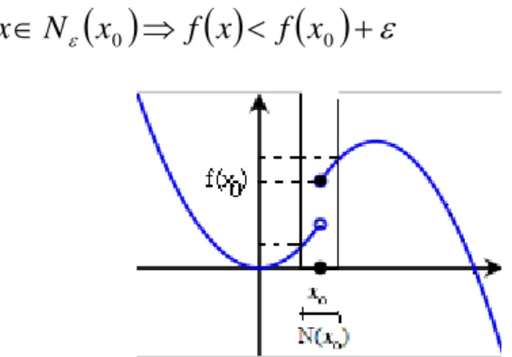
Figure 4.2-1 Best strategy curve for a game with continuous action space . 33 Figure 4.2-2 The -neighborhoods ... 34

Figure 4.2-3 An upper-semi continuous function ... 36

Figure 4.2-4 One dimensional case(fixed point)... 37

Figure 4.2-5 Fixed point for set-valued function ... 37

1

1. Introduction

1.1 Background

Within the rational planning framework, transportation forecasting is important to transportation management. It followed the sequential four-step model or urban transportation planning (UTP) procedure. The four steps of the classical urban planning system model includes Trip Generation, Trip Distribution, Modal Split process, and Traffic Assignment.

Traffic Assignment Problem(TAP) is a multicommodity flow problem which arises when users (or commodities) must share a common resource, the street network. It is to assign flows by various modes in given link to paths in transportation networks. It describe how road-users to choose the optimal route between an origin-destination (OD) pairs, and can be used for analyzing and forecasting traffic flows on every link or route furthermore. However, each user’s choice is dependent upon other users’ choices as well, because the travel time on each street depends on the total number of cars on that street: more congestion means longer travel times. Meyer and Miller (2001) introduced several traffic assignment techniques as follows:

(1) Static assignment model

Network flows will not vary with time in the above approaches. In static assignment techniques, these procedures assume that each vehicle is

simultaneously located on every link on its chosen path and assign all flow simultaneously to all links on the chosen paths. The commonly static assignment technique as follows:

2

 All-or-nothing assignment: It is the simplest approach involving the selection and loading between each origin and destination. It makes a previous assumption that road capacity is unlimited, and link cost is fixed. For each OD pair, find the shortest path and assign all the travel demand into it. The method ignores the limitations imposed by restriction on the capacity of the network. Links may be allocated far greater flows than they are capable of carrying.

 Equilibrium assignment: The idea of equilibrium in the analysis of

transportation networks arises from the dependence of the link travel time on the link flows. Travelers will strive to find the shortest path (least resistance) path from origin to destination, and network equilibrium occurs when no traveler can decrease travel effort by shifting to a new path. In this situation, no user can changing travel path unilaterally to reduce the travel cost or time.

 Stochastic assignment: The second assignment technique is also called deterministic user equilibrium, because it assumes all travelers obtain perfect information on travel costs on any given path are perfect, resulting in making rational route choices. However, in real world, traveler cannot always obtain the whole network information. This leads to development of stochastic assignment, in which link travel time function is viewed as random variables varying with users’ preferences, perception and experience.

3

In real world, the static representation of network performance is not sufficiently accurate. A dynamic representation of route choice behavior and resulting network performance is required in which the movements of vehicles along their chosen paths is explicitly simulated through time. Dynamic assignment models may be either probabilistic in terms of the simulation of users’ route choices and/or determination of vehicles’ travel times along given links, or they can be deterministic.

It is unrealistic assumption obviously, but for many regional transportation

planning applications, static assignment assumption is acceptable and can yield useful results. The research use the game theory to analyze the equilibrium assignment which is classified in static assignment.

1.2 Research Objective

Game theory aims to help people understand situations in which decision-makers interact. It had been applied in transportation in many different aspects. Fisk (1983) discuss some transportation problem as the game theory models, include Nash non-cooperative and Stackelberg games. The discussion serves to underline differences between two categories of transportation problems and introduces the game theory literature as a potential source of solution algorithms. The purpose of research is to demonstrate why the n-person assignment problem can be regard as a two-person game. The research construct a n-person non-cooperation game, use the technique of game theory to consider the assignment problem. Then prove the equivalent between the constructed n-person concave game to a two-person zero sum

4

game. The research use the idea proposed by Zukhovitshii et al. (1973), demonstrate the theory step by step.

1.3 Research Procedure

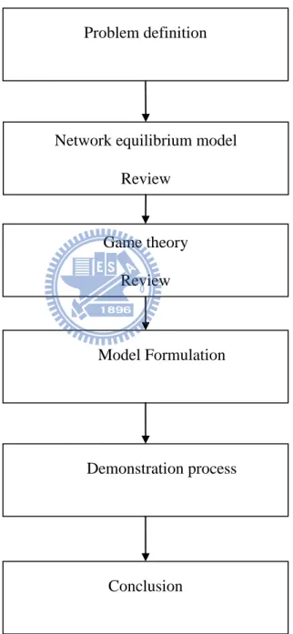
Figure 1.3-1 is the procedure of the research

Figure 1.3-1 The research flow chart

Network equilibrium model Review Game theory Review Model Formulation Demonstration process Conclusion Problem definition

5

The research was divided in following part: (1) Problem definition:

This paper tends to make a completely proof that the network traffic assignment problem can be represented in a n-person concave game, which is equivalent to a two-person zero-sum game. It can help us analyze the problem in different way.

(2) Review:

Before we start to discuss the traffic assignment game, we first review the existed assignment model. Chapter 2 review the article about network

equilibrium, include the development of the equilibrium model and their foundation concept. Because of changing our view to the game based side, Chapter 3 reviews the basic theory of game, and introduces the application of game theory to the traffic side.

(3) Model Construction and Demonstration:

In Chapter 4, we first construct a network game, and use several mathematic theorems to demonstrate the element of the game, include the existence and uniqueness to the equilibrium point. Then make the demonstration to prove the equivalent to the n-person game with two person game.

(4) Conclusion and contribution

Finally, this paper presented some conclusions of this literature and the contribution for the traffic field.

6

2. Network equilibrium model

This section reviews principle of the equilibrium in network, and the development of mathematic model of traffic equilibrium network.

Notation definition: N : Node set A: Arc(link) set P: Path set j i, : Node i,node j, i, jN : a Arc (link)a, aA p: Path p, pP ij

P : The set of all path between node iand node j, i,jN

a c : Arc cost p c : Path cost a f :Flow on arc a

f : The set of all arc flow , f 



f₁, f₂,..., f_a,...



p

h : Flows on path p

7 ij

u : The minimum cost between node iand node j, i,jN

u: The set of all O/D pair, u 



u₁₁,...,u_ij,...



ij

T : Demand of the origin i to destination j

T: The set of all demand of different OD pairs, T 



T11,...,Tij,...



ap

 : Indicator variable, _ap 1 if arc a path  p; _ap 0, otherwise

: Arc/ Path incidence matrix.

: O/D path incidence matrix

2.1Principle of User behavior

The network equilibrium is a nonnegative flow pattern occurring on a given network which is consistent with marketing clearing (i.e. with supply equals demand in either the transportation market or in the underlying commodity market) or flow conservation (Friesz, 1985). It is the main concept of the traffic assignment model. To find the network equilibrium, the first thing is to introduce several concepts

presented by Wardrop(1952).

Wardrop(1952) assume that users have full information , and give the conclusion to the principle of user behaviors as below:

(1). The journey times on all the routes actually used are equal, and less than those which would be experienced by a single vehicle on any unused route (2). The average journey time is a minimum value.

8

In Wardrop’s first Principle, each user non-cooperatively seeks to minimize his cost of transportation. The traffic flows that satisfy this principle are usually referred to as "user equilibrium" (UE) flows, since each user chooses the route that is the best. Specifically, a user-optimized equilibrium is reached when no user can lower his transportation cost through unilateral action.

To define the user equilibrium, the flow pattern satisfying the following conditions: h_p



Cp

 

h u



0, 



i, j,pPij



(2.1-1)

 

 ij 0 p h u C , 



i, j,pPij



(2.1-2)

 

0 



 u T h ij P p p ij , 

 

i,j (2.1-3)



  p p ap a h f  0 a (2.1-4) 0  h (2.1-5) 0  u _(2.1-6) Expressions (2.1-1) and (2.1-2) above are readily recognized as equivalent to Wardrop’s first principle, which require that for utilized paths between a given origin - destination pair, path cost equals the minimum path cost; paths whose costs exceed that minimum are not utilized. This principle conform the actual user behavior, can be applied on the assignment issue on roadway network.

The second principle is implies that each user behaves cooperatively in choosing his own route to ensure the most efficient use of the whole system. Traffic flow satisfying Wardrop's second principle is generally deemed "system optimal" (SO). Economists argue this can be achieved with marginal cost road

9

pricing. The system optimal equilibrium only attach when all user cooperate to choosing route, therefore, it’s not adapted in the real urban network. The most application of system optimal is in the other system, like railroad, marine transportation and air transportation field.

2.2 Mathematic model

This part introduces the manly mathematical model development of the traffic assignment problem.

2.2.1 Mathematical Programming

Beckmann et al. (1956) formulate a Mathematical Programming (MP) model to find the Wardrop’s equilibrium. The model assumes that the cost-flow function of link can be separable. In other word, the link cost only influenced by the object link flow. The model successfully show that original network equilibrium problem could be transformed into an equivalent optimization problem: if the cost on any link is a function of the flow and of no other flows, then the flows satisfying user equilibrium principle are unique and are the same as the following minimize a specified objective function. ) ( min Z f f (2.2-1) =



a f a f a dx x C 0 ( ) min (2.2-2)   f t s .. (2.2-3) } 0 , , {       f f h h T h (2.2-4)

10

By the K-K-T condition of the above non-linear programming, we can find the necessary condition of this mathematic programming model, the following function are K-K-T condition 0 ) (cp uij hp  pPij i,j (2.2-5) 0   ij p u c (2.2-6)

The above model follows the Wadrop’s first principle. Equation (2.2-5) and equation (2.2-6) plus the constraint equation (2.2.1) and equation (2.2-4) equal to the equation (2.1-1) to (2.1-4). Therefore we can transfer the original network equilibrium assignment problem to mathematic programming model as above form. We can also transfer equation (2.2-5) and equation (2.2-6) to following formulation:

If h_p 0c_p u_ij pP_ij i,j (2.2-7)

If c_p u_ij h_p 0 pP_ij i,j (2.2-8) Equation (2.2-7) describe that if the path pfrom origin node i to destination

node jis already be used ( i.e. flow on path h_p 0 ) , the travel cost is equal to the minimum travel cost from origin node i to destination node j. Equation (2.2-8) describe that if the travel cost on path p more than the minimum travel cost from origin node i to destination node j, then the user would not use the path p (i.e. flow on path hp 0) .

Beckmann (1956) assumes that link travel cost is separable. In fact, if we consider different direction on crossroad, the link travel cost will be affected by the

11

other links’ flow, and each link has different weight effect to another. Therefore, the assumption which assumes the dividable link cost is unreasonable. Dafermos (1972) assumes that the Jacobian matrix of link travel cost is symmetrical. This assumption allows the link cost function contain the influence of flow on other links.

Take A and the B two link sections as the example, the influence on B which is affected by the unit increase (or reduction) flow on link A, must be equal to that the influence on A which is affected by the unit increase (or reduction) flow on link B. The following equation can explain the situation:

a b b a f f C f f C      ( ) ( ) (2.2-9) However, a speaking of intersection, if the links nearby the objective link have different link width, the level of influence will be different. Even if the links nearby the objective link all have the same link width, if the marginal cost function which is affected by the other impact factor of the cost function is different, that is, the marginal effect cause by the increase unit are different. Thus, the assumption that equation (2.2-9) express will be unreasonable.

Dafermos (1980) relax the assumption that link travel cost is separable, transfer the network equilibrium model into following linear integral form:



a a h f C x dx f ) ( 0 min , (2.2-10)

In equation (2.13), the impact factor to link cost, not only include the current flow on itself, but also affected by the flow on the other related links. The equation (2.2-10) is formulated to vector integral form, therefore, we must define its integral path first,

12

and different definition of integral path will be different resolve. Hence, the equation (2.2-10) is not a complete definition mathematical model. The model which has objective function (2.2-10) is unable to solve.

2.2.2 Nonlinear Complementarity Problem

Aashtiani (1979) drop the assumption that link travel cost is separable, proposed that the assumption to take the path as variable to formulate mathematical model, which is called the Nonlinear Complementarity Problem (NCP). This model ignores the assumption of link cost function assumed by Beckmann and Defermos. The main assumption of NCP problem which is assumed that path as variable, however, in the real world, the network problems have great amount of paths, it will make the model become too complex to solve. Thus, NCP problem is not adapted to solve the large scale network problem. Li (1987) also proposed that NCP model can’t be convergence to great accuracy in some network type. The model formulation is as following:



cpuij



hp 0 pPij i,j (2.2-11) 0   ij p u c (2.2-12)   h (2.2-13) } 0 , {      h h T h (2.2-14) By above equations we can find that the resolution from NCP problem is also satisfied the network equilibrium K-K-T condition. So that we can use NCP formulation to describe the network traffic assignment problem. Though the above

13

equations are similar with equation (2.2-5) and equation (2.2-6), it cost function have less assumption than mathematic programming model which 2.2-1 mention.

2.2.3 Variational Inequality Problem

Smith (1979) and Dafermos (1980) proposed another model which is called Variational Inequality Problem (VIP). The model also relaxes the assumption that link travel cost is separable proposed in Beckmann’s model. Take link (Smith) and path (Dafermos) as variables to construct the VIP model. Tobin (1986, 1987, 1988) Friesz (1990), and Kyparisis (1987) all make the sensitivity analysis to this model. The model can express as following:

find the solution f*, which is satisfied the following equation

0 ) )( (f* f  f*  c for all f  (2.2-15) which } 0 , , {       f f h h T h

2.2.4 Fixed Point Problem

Kuhn (1968) proposed the Fixed Point problem (FPP). All model mention above (MPP, NCP, VIP) can be transfer to a FPP problem as following equations:

)) ( ( p p ij p h c u h    pPij i,j (2.2-16) 0 ) (cpuij  pPij i,j (2.2-17)



   ij P p ij p T h 0 pP_ij i,j (2.2-18)

14

The equation(h_p (c_p u_ij))Max(0,h_p (c_p u_ij))

i.e. h_p 0

2.3 Summary

In this chapter, we first introduce the Wardorp’s principle of the user behavior, which is the important basic concept in our model. In the second section, we list the several mathematic program models in the traffic assignment field, which formulate the model in diverse ways: as a nonlinear complementarity problem, a fixed-point problem, a system of nonlinear equations, and as variational inequality.

15

3. Game theory

Game theory is the important tool when people face the competition. It can help people to analyze the situation to decide the strategy which he/ she should take when he/ she need to make a decision to compete with his/her competitors. Situations modeled as games typically involve several parties having different interests, who need to decide how to behave. The level of benefit that each party gains depends not only on its own actions, but also on the choices of the other parties. The mathematical formulation of all games is similar, either explicitly or implicitly, to an optimization problem that includes more than one objective, and the decision variables are shared by the different objectives. Defining a game requires identification of the players, their alternative strategies and their objectives. Formulating a problem as a game is worthwhile if the solution, such as Nash equilibrium or Stackelberg equilibrium, leads to new insights on the analyzed problem.

3.1 Development of Game theory

The first known discussion of game theory occurred by James Waldegrave in 1713. Cournot (1838) publicated a general game theoretic analysis, considers a duopoly and presents a solution that is a restricted version of Nash equilibrium. But the major development of the theory began in the 1920s with the work of the mathematician Emile Borel and the polymath John von Neumann (1928). A decisive event in the development of the theory was the book public by Von Neumann and Morgenstern (1944), which established the foundations of the field. In the early 1950s, Nash’s (1950) Ph.D. thesis, 28 pages in length, introduces the equilibrium notion now known as “Nash equilibrium” as the following equation

16



 

*



1 * 1 * * , , : , ,   _  _ i xi Si xi xi fi xi x fi xi x

Nash equilibrium is a solution concept of a game involving two or more players, in which each player is assumed to know the equilibrium strategies of the other players, and no player has anything to gain by changing only his or her own strategy unilaterally. If each player has chosen a strategy and no player can benefit by

changing his or her strategy while the other players keep their unchanged, then the current set of strategy choices and the corresponding payoffs constitute a Nash equilibrium.

Game theory is the most popularity tool when people tend to make the decision in competition. The next section will introduce the application of the game theory in the transportation field.

3.2 The application of game theory in transport field

This part introduces the application of game theory in the transport application. Colony(1970) formulates a route choice problem as a zero-sum game. One of the players is a driver that chooses whether to use an arterial road, the other is an imaginary entity which chooses the level of service on the road, and tries to disturb the driver’s journey. Rosenthal (1973) and James(1998) formulates a general game between n- individuals who choose the road segment out of a given set, where the cost of each road segment increases if more individuals choose it. The former formulated a programming problem, which solution is always a pure-strategies Nash equilibrium of the game, and shown that a solution always exists. Fisk(1984) mentions that the user equilibrium principle, introduced by Wardrop(1952), is in fact a game since it meets the conditions of Nash equilibrium. Van Vugt et al. (1995) present a two-player

17

strategic form game, where each player chooses either car or public transport. The conclusion is that the selfish way travelers make their choices is bad for everyone, that is , the

prisoner's dilemma in game theory.

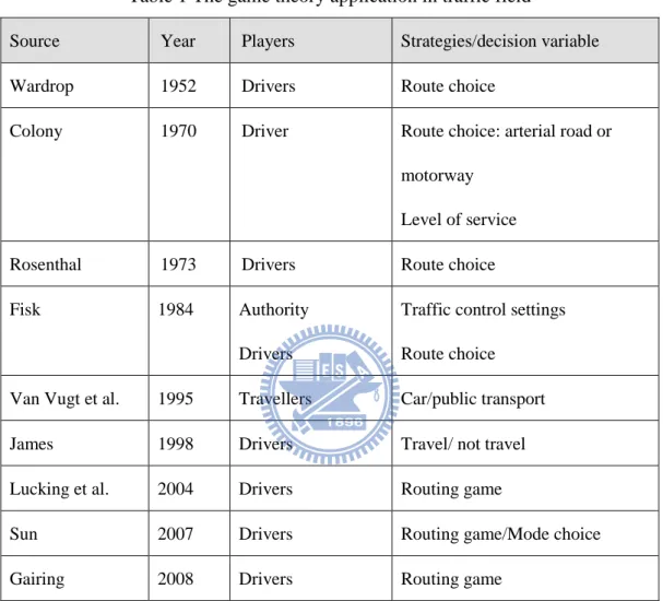
Table 1 The game theory application in traffic field

Source Year Players Strategies/decision variable

Wardrop 1952 Drivers Route choice

Colony 1970 Driver Route choice: arterial road or motorway

Level of service Rosenthal 1973 Drivers Route choice

Fisk 1984 Authority

Drivers

Traffic control settings Route choice

Van Vugt et al. 1995 Travellers Car/public transport

James 1998 Drivers Travel/ not travel

Lucking et al. 2004 Drivers Routing game

Sun 2007 Drivers Routing game/Mode choice

Gairing 2008 Drivers Routing game

In the recent paper, Sun(2007) construct a urban transit non-cooperative static game, and assume the prefect information, to find the generalized Nash equilibrium, which is to describe both the competitions among different transit operators and the interactive influences among passengers. Lucking et al. (2008) use the concept of Nash equilibrium to construct a self routing non-cooperative network model. In the hybrid model which consist of KP model and Worst-cast model, each of n users is using a mixed strategy to ship it unsplittalbe traffic over a network consisting of m

18

parallel links. Gairing et.al (2008) use the simaliar concept to discuss a discrete routing game.

3.3 The Non-cooperative Game

From the Wardrop’s principle, the concept of user equilibrium, every user

pursuit one’s maximum utility (we can also said, minimum travel cost). We know that users all non-cooperative to pursuit one’s maximum utility. That is, the character of the route choice game is non-cooperative game. By this reason, the application of game theory in transportation field almost non-cooperative game.

Game theory is divided into two branches, co-operative and non-cooperative game theory. The distinction can be fuzzy at time but, essentially, in non-cooperative game theory the unit of analysis is the individual participant in the game who is concerned with doing as well for himself as possible subject to clearly defined rules and possibilities. In comparison, in co-operative game theory the unit of analysis is most often the group or, in the standard jargon, the coalition; when a game is specified, part of the specification is what each group or coalition of players can achieve, without reference to how the coalition would effect a particular outcome or result.

N.N. Vorb’ev(1977) give this kind of game a briefly definition:

   

Si i I Hi i I I _{ }   , , (3.3-1) i

S represent the situation

S is the situation set, and



  I i i S S .

19

 

s

H_i is the payoff function of player i in the situation s.

i

H represent the payoff function of player i.

Iis the player set.

Definition 3.3-1: Let a constantc, for sS, we define constant-sum game if the following game exist

 

S c H I i i 



 _(3.3-2) If c0, We called this type of game zero-sum game.

3.4 summary

We aim to use the view of game theory to analyze the network assignment process. First we have to understand the basis concept of the game theory. In this chapter briefly reviews the game theory, and introduces the history of the game theory. The second part of the chapter review the application of game theory in the issue relate to traffic assignment problem. Most of them is a concept game assume a entity which aims to reduce the user’s utility. The last part of the chapter introduces several important definition of game. We define the Nash equilibrium, the non-cooperative game, and the zero-sum game, which are the special cases in constant game.

20

4. Model Construction and Demonstration

In this Chapter, we start to consider the traffic assignment problem by the game theory. The flowchart of demonstration process is below

Figure. 4.1-1 The flowchart of the demonstration process

4.1Network Game Definition

In this section define some foundation concept and the definition to the demonstration process.

Because of the concept of the user equilibrium which is introduced by Wardrop, the network equilibrium is a concave n-person non-cooperative game that every user tends to gain their maximum utility.

Equal to two-person zero sum game Saddle Point

“=“ of VIP

Uniqueness of equilibrium point Existence of equilibrium point

compact set

Pay –off function can be formulated as VIP form pay-off function of N-person Game is pseudo concave

21

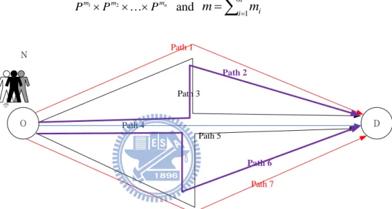
4.1.1 Problem region

The network concave n-person game to be considered is described in terms of the individual strategy vector for each of the n players. The strategy of the ith player is represented by x which chose from the path set _{i P}mi_{, i}_1,...,n

,which is the path in the target Network. The vector m

P

x then denotes the simultaneous strategies of all players, where Pm is the product space.

n m m m P P P 1 2 _and



  n i mi m 1 O D Path 1 Path 2 Path 3 Path 4 Path 5 Path 7 Path 6 N 人 事

Figure 4.1-2 The graph of network game

Players choose the paths pj which they use to gain the maximum utility, so the

strategy set of the ith player is x_iX_i 



p₁,p₂,...,p_m



,i1,...,m is the number of path in the same OD. Let K be the user/path instance matrix, we have

p h x K  f h 

22

The allowed strategies will be limited by the requirement that the selected x_,

which can transfer to the link flow f by the above process, satisfied the convex, closed, and bounded set

} 0 , , {       f f h h T h

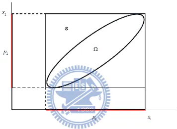
Denote the path pj of ,then we have a bounded product set S , n

x x

x

S ₁ ₂ . The figure 4.1-3 illustrate for n2.

Figure 4.1-3 The region of the game

4.1.2 Payoff function and some basic theorem

The payoff function for the ith player depends on the strategies of all the other players as well as on his own strategy, and is given by the function

 

i



i n



i x  x1,...,x,...,x

 

23

If we know the link cost function c

 

f , we can use the instance matrix  to find the path cost function Tc

 

f C_p, then we can know the cost function C_p

By the hypothetic of the network game, users tend to gain their maximum utility is equal to find the minimum cost path of the OD pair, so we can say that

 

x MinC

 

x Max i p i  

 

x Max



C

 

x



Max i p i   

Now we consider the definition of equilibrium of network game.

Definition 4.1-1: Assumed that xS,_i

 

x is continuous in x and is concave in

i

x for each fixed value of



x₁,...,x_i1,x_i1,..,x_n



, that is , the i-th player under selection by the other players’ strategies . With this formulation an equilibrium point of the n-person concave game is given by a pointx*, such that

 







 

* *







1 * * 1 * ,..., ,..., | ,..., ,..., max _{i i n i n} y i x x y x x y x i   i1,...,n (4.1-1)

At such a point no player can increase his payoff by a unilateral change in his strategy. The idea of the equilibrium point for the concave n-person game was first presented in Nash (1961).

Definition 4.1-2: Assumed that the function 

 

x,y defined for

 

x,y  by

 

_





   n i n i i x y x y x 1 1,..., ,..., ,  (4.1-2)

24

Observe that for

 

x,y  have



x₁,...,y_i,...,x_n



S, i 1,...,n, so that

 

x,y

 is continuous in x and yand is concave in y for every fixed x. The point *

x , for which











 





 x*,x* max x*,y |y

Which is call a normalized equilibrium point ( NEP) for the game that mention by Rosen (1965). It is easy to see that every NEP is also an ordinary EP. However, equilibrium points exist which are not normalized.

NEP helps people consider the problem in the general way. They can have different weight factor with the same payoff function. Then the equation (4.1-2) can be formulated as below

 

_





   n i n i i i x y x r y x 1 1,..., ,..., ,  (4.1-3) The concept can be applied in the network game, the people in the network game who choose the same path may have different effect to the network system. For example, the truck user brings more influence then the car user.

By the definition of the payoff function, _i

 

x is concave with respect to the fixed pointx. Combined with the definition of function 

 

x,y , we know that

 

x,y

 is also concave with the fixed pointx.

Now we define the gradient function g

 

x of 

 

x . Consider the vector function below:

25

 

 

 

 

 

_                n nm n n n m x x x x x x x x x g  ,...,  ,...,  ,...,  1 1 1 11 1 1 _(4.1-4)

Assume that all the derivatives exist and are continuous. Obviously,

 

x y

 

x y y x

g   , 

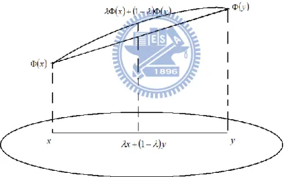
Definition 4.1-3: Let g:Em, where  is a nonempty convex set in En_{. The}

function  is said to be concave on  if x,y, 





 

0,1, we have







x  y



 

  

x  

  

 y





1





1



(4.1-5)

Fig 4.1-3 Geometric interpretation of Definition 4.1-3

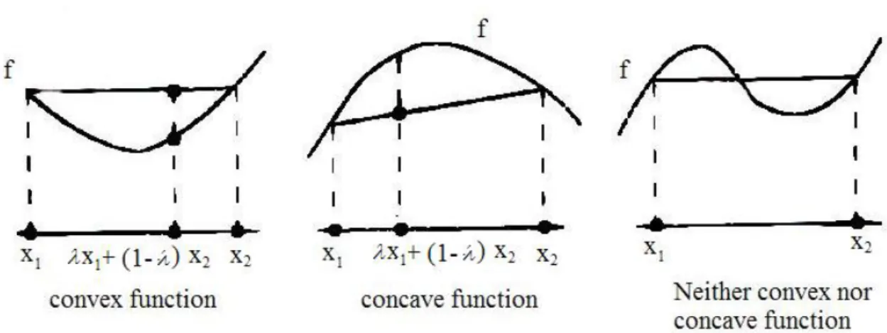
The above graphic is the geometric interpretation to the Theorem. Then the following figure briefly show the different type function relate to the theorem.

26

Figure 4.1-4 Convex and concave functions (graph from Bazaraa et.al(2006))

Theorem 4.1-4：Set  be a nonempty convex open set inEn, and let



:





E

m. Andg is said to be differentiable on . Then  is concave if and only if for any

  y x, , we have

 

y 

 

x 





 

x

 

T yx



 _(4.1-6) Similarly,is strictly concave if and only if for anyx,y, we have

 

y 

 

x 





 

x

 

T yx



 _(4.1-7) Proof:

(Necessary)

Suppose that  is concave, let





 

0,1 x,y, and we set that ) ,..., , (x₁ x₂ x_n x ) ,..., , (y₁ y₂ y_n y

27

So we can get the gradient function

 

_                  n x x x x x x x ( ), ( ),..., ( ) 2 1

 

_                      ) ( )( ), ( )( ),..., ( )( ) ( 2 2 2 1 1 1 n n n x y x x x y x x x y x x x x y (4.1-8)

by Definition 4.1-3, we have equation (4.1-5)







y  s



 

  

y  

  

x 



1





1



Then we get







x yx



 x   y  

 

x 



( )



( )



(4.1-9)

is differentiable, then we can get the gradient function:









 







n n



n n n n x y x y x y x x x y x x x x y x                           ( )( _{1 1}) ... ( )( ) _{1 1 1} ... 1 (4.1-10) Let ₁,...,_n 0(when 0), then take (4.1-10) into (4.1-9), we have



y x





y x



y

 

x x y x x x y x x n n n n n n                    _{     } ) ( ... ) ( ) ( ... ) ( ) ( 1 1 1 1 1 1 (4.1-118) Set 0, and let (4.1-11) divided by , and set 0, then we get

 

x y x y x x x y x x n n n               ) ( ) ( ) ( ... ) ( ) ( 1 1 1 (4.1-12)

28

Observe the left hand side of equation (4.1-12), it is equal to (4.2-8), then we get



yx

  

x (y)

 

x

 

x y x



x y      ( ) ( )

The proof of necessary is complete.

In above equation, if we take the equality away, we can get the proof of strictly concave function.

(Sufficiency)

Let x,y,





 

0,1 , we set that







   x y z



1



(4.1-13)

 

z 





x









y



 1 (4.1-14)

And By the hypothesis of the theorem, we have

   

x  z 

 

z xz



 (4.1-15)

   

y  z 

 

z yz



 (4.1-16)

Let (4.1-15) multiplied by , and (4.1-16) multiplied by



1





, then we get

 

x  

 

z  

 

z xz









29



1



   

 y  1



   

z  1



  

 z yz



(4.1-18)

Plus equation (4.1-17) to equation (4.1-18), we can get

  

x  1

  

 y  

  

z  1

  

 z  

 

z xz

 

 1

  

 z (yz)















(4.1-19) Consider the right hand side of equation (4.1-19)

  

z 1

  

 z  

 

z xz

 

 1

  

 z (yz) 









 

z 

 

z



x







yz



 



1



 

z 

 

z zz



 

 

z 





x









y



  1

Then consider the equation 4.1-19, we have

  

x 1



  

y





x



1





y



)



      

By Definition 4.1-3, 

 

x is concave. The proof of sufficient is completed. Q.E.D.

Theorem 4.1-5: when 

 

x _{function is (strictly) concave, the gradient function}

 

x

30

   



g x g y,yx



0,

 

x,y ,x y _(4.1-20)

Proof:

i. If strictly is untenable, that is, proof



g

   

x g y

 

T yx



0

Set 

 

x _{be a concave function, let} x,y_{, by Theorem 4.1-4, we know that}

the following relation:

 

y 

 

x 





 

x

 

T yx



 _(4.1-21)

 

x 

 

y 





 

y

 

T xy



 _(4.1-22) Plus equation (4.1-21) and equation (4.1-22), we can get

 

x 

 

y 

 

x 

 

y 





 

x 

 

y

 

T yx



 _(4.1-23)

Then

 

 



 x  y

 

T yx



0

By the definition of g

 

x _{(equation 4.1-4)}

   



g x g y

 

T yx



0

Q.E.D.

ii. If strictly hold, that is, proof



g

   

x g y ,yx



0

 

y 

 

x 

  

xT yx



31

 

x 

 

y 

  

y T xy



 (4.1-25) Plus the above equation (4.1-24) and equation (4.1-25), finally we can get

 

 



 x  y

 

T yx



0 Then

   



g x g y

 

T yx



0 _(4.1-26) Q.E.D.

4.1.3 The VIP network model

From the chapter 2, we have the foundation Variation Inequality network model, to find the solution f*, which is satisfied the following equation

0 ) )( (f* f  f*  c for all f  } 0 , , {       f f h h T h

 

f

c is strictly monotone function. It can be represent in the following type

  

,  )



0



 x y T y x

The above equation can be transfer in following equation

 

 



 x  y

 

T yx



0

32

We take the path flow as variable to construct the network game. Now, let x y, because c

 

h is strictly monotone function, The equality of above equation will be refused. We have 0 ) )( (h* hh*  c _(4.1-29) The above equation matches the character of strictly concave and can be represented as below:

  

,  )



0



 x y T y x

It can easily find that the equation of network model match the gradient of the network concave game we assume.

Now we face the problem that the amount of path is a large number that is too hard to solve. Smith (1979) proposed a equivalent to the VIP form which take the path and link as variable. As the following equation :

 

h h Cp

 

hhp c  



 



Ca f ap



hp



 

 









 C_a f _aph_p

 



 C_a f f_a

 

f f c  

By the above theorem, we can also take link flow as variable to consider our network game .

33

4.2 The existence and uniqueness of network game

This section proves the existence and uniqueness of the network assignment model. The method of proof is essentially a rearrangement of Rosen’s (1965) proof for existence and uniqueness of equilibrium point of the concave n-person game.

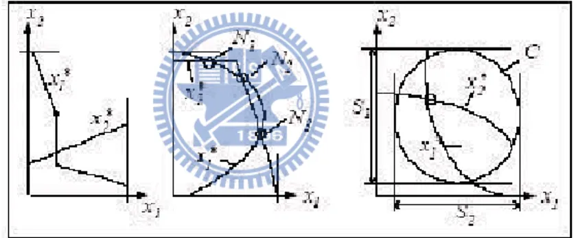
In the former section, we assume that the network game is a concave n-person game, and proof that the variation inequality model matches the assumption of the game. By the preliminary concept of game, the equilibrium point (EP) of the game might have three situations. It is possible to have no equilibrium, several equilibria, or one unique equlibrium. For instance, the figure 4.2-1 show the situation of EP of two person game.

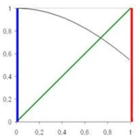
Figure 4.2-1 Best strategy curve for a game with a continuous action space(Krishnan,2006)

We are interested in a subset of continuous games that have a unique equilibrium. It turn out that a set of games that can satisfy this criteria is concave game.

By the reason of above, we want to prove the existence of the equilibrium first, and second, we prove the uniqueness of Nash equilibrium in this network game.

34

4.2.1 Existence of equilibrium point

From section 4.1, we define the payoff function



 

x and the function 

 

x , by the equation 4.1-2, 

 

x,y is continuous in x and yand is concave in y for every fixedx.We now prove the existence theorem for the concave n- person game.

Definition 4.2-1: A single-valued mapping f :X Y sends a point x of X to a point f

 

x of Y. But on some occasions, we need to consider a mapping f that lets correspond to each point x of X a subset f

 

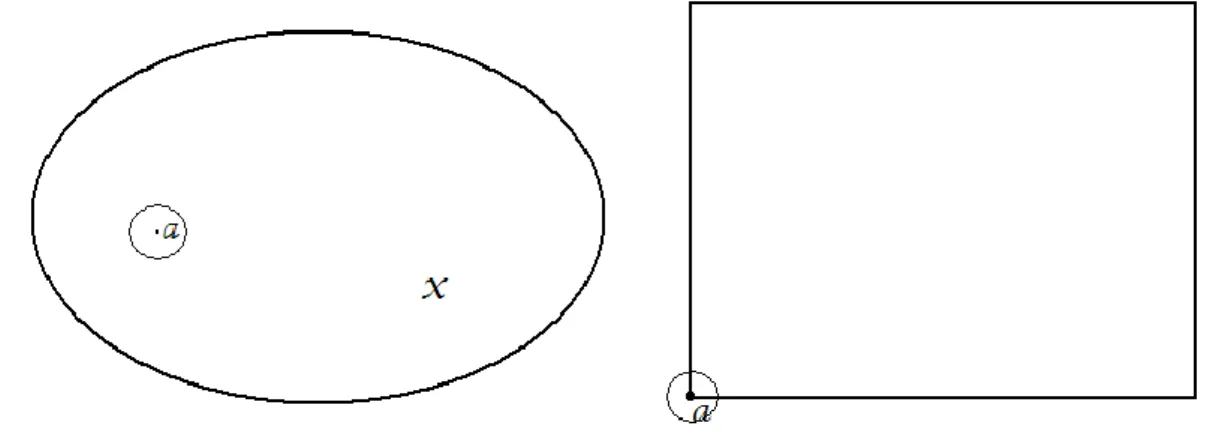
x of Y. Such a mapping is termed a set-valued mapping or a point-to-set mapping.

Definition 4.2-2: An -net of a metric space X is a finite subset



ai |i1,2,...,s



of X such that the family of  -neighborhoods



N

 

ai, |i1,2,...,s



is a covering of X . Here, N

 

a, 



x|dis

 

x,a 



denotes an -neighborhoods inX .

Figure 4.2-2 The -neighborhoods

Definition 4.2-3: A set X is compact if any sequence of its points contains a sub-sequence that converges to a point in X .

35

Corollary 4.2-4: If a metric space X is compact in the sense of definition 4.2-3, it has an -net for any  0.

Proof. Suppose that X had no  -net. Take any one point 1 a .

Since there is no -net, the -neighborhoods N

 

a1, cannot coverX . So that some a2X does not belong to N

 

a1, .

Again, for the same reason, there is some a3 belonging to none of N

 

a1, and

 

a2, N .

Continuing this procedure, we obtain a sequence

 

av such that

 

, 1 1 v v i v a N a



  _ . By construction, the sequence has the property dis



au,av



 for uv. Such a sequence has no convergent sub-sequence, contradicting the compactness of X ,

Q.E.D.

Definition 4.2-5 (convexity): A vector y in Rn is said to be a convex combination if y can be written as



  s i i ix y 1 



  s i i 1 1  , _i 0 , for i1,...,k (4.2-1)

Definition 4.2-6: If X are convex subsets in _i n

R



i 1,2,...,s



, their linear combination



 n i i iX 1  is also convex.

36

Definition 4.2-7: (upper semi-continuous)

(a) Point : A numerical function defined on X is said to be upper semi-continuous at x , if, to each ₀  0, there corresponding exist a neighborhood N_

 

x₀ such that

 

   



   

N x₀ f x f x₀

x (4.2-2)

Figure 4.2-3 An upper-semi continuous function

(b) Mapping: Let  be a mapping of a X Y. Let x be a point of ₀ X . We say

 is upper semi-continuous at x if for each open set G containing ₀ x_o there exists a neighborhood N_

 

x₀ such that

 

x x G

N

x _{ 0}  

Corollary 4.2-8: (Brouwer, 1909,1910). Let X be a nonempty compact convex set in

n

R , and f :X X be a continuous mapping that carries a point x of X _to

37

Figure 4.2-4 One dimensional case(fixed point)

Theorem 4.2-9: (Kakutani, 1941). Let X be a nonempty compact convex set in Rn, and f :X 2X be a set-valued mapping which satisfies

(a) For each xXthe image set f

 

x _{is a nonempty convex subset of} X ;and (b) f _{is a closed mapping}

Then f has a fixed point.

Figure 4.2-5 Fixed point for set-valued function

Proof. Since X is compact, recall the Corollary 4.2-4 on the existence of  -net , for every  0, it has an -net N 



ai |i1,...,s



. Next choose an arbitrary point i

b of f

 

ai . Then, we define the continuous functions _i

 

x on X by

 

max



i ,0



i x x a

  _

38

According to Definition 4.2-2, Since N an _  -net, for each x we have

i a x 

   for some i, so that we have _i 0 for this i. With these function we can obtain the weight functions

 

 

 



        s j j i i x x x w 1



i1,...,s_



(4.2-3)

Using these weight function, we define a single-valued continuous mapping

 

_

 

      s i i i xb w x f 1 X bi



i1,...,s_



 

x 0 w_i ,



w_i 1 (4.2-4) Because of the convexity of X which define in Definition 4.2-5. Then we obtained a single-valued continuous mapping f :X X for every  0. By the Brouwer fixed-point theorem (Theorem 4.2-6), there is a fixed point x,

 

   x f x  _(4.2-5)

Now apply equation 4.2-5 to a sequence

 

_v of positive numbers with limit _v 0. Since X is compact, the correspoinding sequence of fixed point

 

xv ,

 

v v v

x f

x    _{contains a convergent sub-sequence with a limit x}ˆ .

Without loss of generality, assume that we have chosen a sequence

 

_v of positive numbers fulfilling following constraints

39 a. lim 0   v v  b. x v x vlim  ˆ  c. xv  fv

 

xv (4.2-6) We tend to show that xˆ is a desired fixed point of f . Consider the set

 

  f x U O  ˆ 







  u u  U | for a  0

If xˆO_ for any  0, we have dis



xˆ,f

 

xˆ



0, which entails xˆf

 

xˆ because f ˆ is closed in

 

x X . The subsequent discussion will clarify that xˆO_ for any  0.

First note that O is an open set containing _ f ˆ . This can be seen by noting that

 

x









 x U

O  

This union taken over all xf

 

xˆ , and also the openness of U .By the definition _ 4.2-6, we know the convexity of O_

f is upper semi-continuous. Since O is an open set containing _ f ˆ

 

x , there is an

-neighborhood V_ 



x| xxˆ ,xX



of xˆ such that f

 

V_ O_. By ()(),we have

2



40

For these large v, wiv

 

x v 0   implies 2     _{  } v v vi x a , so that x x x a x avi  ˆ  vi  v  v  ˆ <   2 2 .

In summary for large v, we have avi V_ for i with wiv

 

x v 0   , which entails

 



 

   O V f a f b vi  vi   . In view of

 



 v v vi i v b x w x    v

x turns out to be a convex linear combination for only bvi lying in O for large _ v. The convexity of O therefore implies _ xvO for large v. Letting v tend to infinity in view of

 

 , we have in the limit xˆ O 2.

The replacement of  by 2 in the resulting relation is due to the possibility that  xˆ , the limit of

 

xv _{, may lie on the boundary of U . }

However, xˆ O 2 for any  0 is equivalent to xˆO for any  0, whence

 

x

f

xˆ ˆ _{in the light of the preliminary discussion above. This completes the proof,}

Q.E.D.

The following part we use Rosen(1965) method to proof the existence and uniqueness of the Equilibrium point.

41

Proof:

Consider the point-to-set mapping xx, given by

 

 



y x y x z



x R z , max , |      (4.2-1) It follows from the continuity of 

 

x,z and the concavity in z of 

 

x,z

for fixed x that  is an upper semi-continuous mapping that maps each point of the convex , compact set R into a closed convex subset of R. Then by the Theorem

4.2-9, there exists a point x*R such that * * x x  , or



x x



 

x z R z , max , * * *     (4.2-2) The fixed point x* is an equilibrium point satisfying equation (4.1-1), which we rewrite below..

 







 

* *







1 * * 1 * ,..., ,..., | ,..., ,..., max _{i i n i n} y x y x x y x x i   i 1,...,n

If we suppose that x* were not be the equilibrium point. Then, say for il, there would be a point x_l  x_l such that x 



x₁*,...,x_l,...,x_n*



Rand ₁

 

x _l

 

x* . Then we have

 

*



* *



,

,x x x

x 

 , which contradicts (4.2-2). Then the proof is completed.

Recall the network game problem, if we assumed the set

 



| 0





 x h x