Electron hopping conduction in highly disordered carbon coils

(1)

November 26, 2002 11:18 WSPC/155-RPBFMP 00076

Review of Pacific Basin Financial Markets and Policies Vol. 5, No. 3 (2002) 417–438

c

World Scientific Publishing Company

Long-run Stock Performance of Equity-Issuing Firms:

The Case of Private Placements in Singapore

Sheng-Syan Chen Yuan-Ze University Kim Wai Ho

Nanyang Technological University Cheng-Few Lee

Rutgers University Gillian H. H. Yeo

Nanyang Technological University

We find that Singapore listed firms which have conducted private placements subsequently experience long-run stock underperformance. The long-run underper-formance is more severe for small firms and firms with a higher book-to-market ratio. This suggests that small firms and firms with poorer growth prospects are more likely to time the issue when the stock is temporarily overvalued. Further more, we find a positive relation between the long-run stock performance and the change in ownership concentration of the issuing firms, which is consistent with the alignment-of-interests hypothesis. We do not find evidence supporting the earnings-management hypothesis.

Keywords: Long-run stock returns; Equity offerings; Private placements; Emerging markets.

1. Introduction

Previous studies show that equity-issuing firms experience significant long-run stock underperformance. For example, Loughran and Ritter (1995) show

Address for Correspondence: Cheng-Few Lee, Department of Finance, School of Business, Rutgers University, New Brunswick, NJ 08903, USA; E-mail: [email protected] The authors wish to thank Reena Aggarwal, Dosoung Choi, David Ding, Jayant R. Kale, Sie Ting Lau, and seminar participants at the 1997 FMA meetings for helpful comments and suggestions. Any remaining errors are the authors’.

(2)

418• Sheng-Syan Chen et al.

that the average annual return during the five years after issuing is only 5 percent for firms conducting initial public offerings (IPOs), and only seven percent for firms conducting seasoned public equity offerings (SEOs), whereas the corresponding average annual return for comparison firms is 12 percent for IPOs and 15 percent for SEOs.1 _{Affleck-Graves and Page (1995)}

report similar long-run stock underperformance in the case of rights issues using data from the Johannesburg Stock Exchange.

Several researchers suggest that the underperformance phenomenon is consistent with the management-timing hypothesis: issuing firms take ad-vantage of transitory windows of opportunity by issuing equity when they are overvalued.2 Other studies show that the market may have been fooled by management manipulating the firm’s earnings surrounding the time of is-sue (the earnings-management hypothesis).3Affleck-Graves and Page (1995) argue that in the case of rights issues, the management-timing hypothesis does not apply because the new shares are offered to existing shareholders in proportion to their existing ownership. They suggest that the stock un-derperformance may be better explained by market cycles or the inability of issuing firms to generate sufficient internal funds to finance future projects. This study provides further evidence on the long-run stock returns of equity-issuing firms by examining firms that conduct private placements in Singapore.4 Our motivations for studying Singaporean private placements are as follows. First, Singapore listed firms typically raise additional equity capital by way of rights issues or private placements. Unlike in the US, seasoned public equity offerings are seldom used in Singapore.5In this study, we focus on private placements because this form of equity issues receives relatively less attention in the literature.

1_{IPO underperformance is also reported in the United Kingdom (Levis, 1993a), Latin}

America (Aggarwal, Leal, and Hernandez, 1993), and elsewhere (Loughran, Ritter, and Rydqvist, 1994). Other studies reporting long-run stock underperformance of SEOs include Levis (1993b) and Spiess and Affleck-Graves (1995).

2

See Ritter (1991), Loughran and Ritter (1995), and Spiess and Affleck-Graves (1995).

3_{See Teoh, Welch, and Wong (1998a) for IPOs and Teoh, Welch, and Wong (1998b) for}

SEOs.

4

Alli and Thompson (1993) reported a negative 24-month cumulative abnormal return for a sample of 44 US unregistered private common stock placements. However, they did not conduct further analysis.

5_{In Singapore, the seasoned public equity market is not well developed relative to the}

rights issue and private placement markets. The Stock Exchange of Singapore Listing Manual does not provide specific rules on primary seasoned equity offering. To date, there were only a very few public issues including the one issued by Singapore Telecom in 1996.

(3)

Long-run Stock Performance of Equity-Issuing Firms• 419

Second, the institutional characteristics in Singapore make it relatively easier for firms to conduct private placements relative to rights issues. Singapore-listed firms that conduct a rights issue are required to prepare a detailed prospectus while those that conduct a private placement are ex-empted from preparing one. In addition, a firm that conducts a private placement would usually obtain a general mandate to issue shares up to 10 percent of the issued capital at an Annual General Meeting of shareholders held prior to a private placement. The general mandate gives directors the flexibility to issue new shares subject to the 10 percent limit without further approval from the shareholders. Thus, once the mandate is granted by share-holders, the firm has the flexibility to choose the timing of the placement.

Third, regulations on private placements in Singapore are different from those in the US. In particular, Singapore private placements are subjected to a 10 percent cap on the issue size, a five percent cap on the price discount, and a restriction on the sale to insiders and five percent to blockholders.6 Since the placement shares cannot be sold to insiders and blockholders, it is likely that insiders time the placement to maximise their wealth.

Finally, our results also have implications for the investment industry as any abnormal post-issue long-run stock returns would imply that the capital market might not be fully efficient. Since Singapore is an important financial and investment centre in Asia,7 the results in this study should be of particular interest to international investors.

We find that our sample of Singapore firms which have conducted private placements experience long-run stock underperformance similar to those re-ported in previous studies on IPOs, SEOs and rights issues. We also show that the post-issue holding period stock return of an announcing firm is pos-itively related to its firm size and negatively related to its book-to-market ratio. These results are consistent with the management-timing hypothesis because smaller firms and firms with poorer growth prospects have greater incentive to issue shares when they are temporarily overvalued. Further, we find a significant positive relation between the long-run stock performance

6

Ho, Chen, Lee, and Yeo (2000) report that these regulations may explain the negative announcement-period return and the reduction in ownership concentration associated with Singaporean private placements. In contrast, Wruck (1989) finds a positive announcement-period return and an increase in ownership concentration for US private equity placements.

7_{Singapore is the fourth largest foreign exchange trading centre in the world, the fifth}

largest trader in derivatives and the ninth-largest offshore lending centre. There are more than 700 financial institutions in Singapore. (Source: The official website of the Singapore central bank, the Monetary Authority of Singapore: http://www.mas.gov.sg.)

(4)

and the change in ownership concentration.8 This evidence is consistent with Jensen and Meckling’s (1976) alignment-of-interests hypothesis. The result is also consistent with the management-timing hypothesis as managers of overvalued firms may choose to dilute their shareholdings more via a place-ment of shares to outsiders. Finally, our results on discretionary accruals do not provide support for the earnings-management hypothesis.

The rest of the paper is organized as follows. Section 2 describes the data and methodology. Section 3 presents the time series evidence on post-issue stock performance. The analysis of post-post-issue stock performance and the examination of earnings management are discussed in Sec. 4. The last section provides some concluding remarks.

2. Data and Methodology 2.1. Data

The sample of private placements are identified from the Annual Factbooks issued by the Stock Exchange of Singapore (SES) from 1988 to 1993.9 The company’s initial announcement is then obtained from the Daily Financial News which are compilations of corporate announcements received by the SES on the preceding day. Private placements with contemporaneous rights issues of common stock or issues of other securities are excluded. The final sample consists of 53 private placements by 47 firms. Table 1 summarizes the number of placements in each of the years over the sample period.

2.2. Long-run stock returns

In this study, we report long-run stock returns up to three years after the announcement date. However, because of data limitation,10 using a

8

Ownership concentration is defined as the total holdings of managers, directors and non-management holdings greater than 5% (Wruck, 1989).

9_{1988 was the first year in which the SES introduced the rules on private placements.}

Our sample period stopped at 1993 because after 1993, the rules were being relaxed as to the issue size and other issuing characteristics, which may have an impact on the results. While the sample period is not long, our results are not affected by the economic cycle. The GDP growth rates in the sample period from 1988 to 1993 are 11.6%, 9.6%, 9.0%, 7.3%, 6.2%, and 10.4%, respectively. These growth rates are not unusually high or low relative to the growth rate of 9.7% achieved in 1987, the year before the sample period, and the growth rates of 10.1%, 8.8%, and 7.5% in the 1994–1996 period, the three years after the sample period.

10_{We obtain the data from the Stock Exchange of Singapore. The data available at the}

(5)

Long-run Stock Performance of Equity-Issuing Firms• 421 Table 1. Distribution of Private Placements by Year of Placement

Year of Private Placement Number of Observations % of Total

1988 2 3.8 1989 10 18.9 1990 12 22.6 1991 4 7.5 1992 5 9.4 1993 20 37.8 Total 53 100.0

Note: This table summarizes the number of private placements in each of the years from 1988 to 1993. There are 53 placements by 47 firms in the sample. The sample is obtained from the annual Factbooks and the daily Financial News issued by the Stock Exchange of Singapore.

three-year window requires some degree of truncation towards the end of the three-year window period.11 Thus, for our detailed analysis, we fo-cus on the two-year holding period returns. As can be seen later, there is no further significant change in stock returns in the third year after the announcement date.

We use three measures of long-run stock performance in this study: cumulative abnormal returns (CARs), holding period returns, and wealth relatives. We compute abnormal returns, CARs and the associated test statistics as in Ritter (1991) and others, and holding period returns as in Ritter (1991), Loughran and Ritter (1995) and Spiess and Affleck-Graves (1995). The holding period return from months 1 to T for each issuing firm i is defined as HP RiT =

QT

t=1(1 + Rit)− 1. The mean and median portfolio

holding period returns are then computed. The holding period return and the mean and median portfolio holding period returns for the matching firms are computed analogously. If the issuing firm is delisted prior to the end of the holding period or has returns data for less than the holding period, the holding period returns of that firm and its matched firm are truncated on the same day. The significance in the difference between the mean of the issuing firms’ holding period returns and the mean of the matched firms’ holding period returns is tested using the standard comparison of means test. We also compute the median difference and the fraction of the offering firms that underperform their matched counterparts. The Wilcoxon signed rank test is used to determine the statistical significance of the median difference.

11

(6)

The significance of the fraction underperforming is tested using a two-tailed non-parametric test of proportion.

Following Ritter (1991), Loughran and Ritter (1995) and others, we de-fine the wealth relative as the ratio of one plus the average holding period return for the issuing firms to one plus the average holding period return for the matched firms. A wealth relative that is less than one shows that the private placement firms underperform the matched firms.

We use four benchmarks to measure long-run stock performance: (i) a size-matched portfolio; (ii) a book-to-market (BM) matched portfolio; (iii) industry indices; and (iv) the value-weighted Stock Exchange of Singapore All-Share Index.12 The size-matched benchmark portfolio is constructed based on the approach adopted in Loughran and Ritter (1995). For each issue, all listed firms are ranked on the basis of market capitalization at December 31 prior to the date of announcement of the private placement. The matching firm is then chosen as the firm with the market capitaliza-tion closest to but higher than that of the issuing firm and does not have a private placement within five years prior to the announcement date of the issuing firm.13If a matching firm is delisted or privately places equity during the holding period, a second (and, if necessary, third, fourth, etc.) matching firm is spliced in after the delisting date or the private placement date of the first matching firm. The replacement firm is the non-issuing firm with the market capitalization on the original ranking date immediately higher than the original matching firm. Five of the sample firms require two matched firms and none require three matched firms.

The BM matched portfolio is constructed using an approach similar to Spiess and Affleck-Graves (1995). The BM ratio is computed as the firm’s book value of equity divided by its market value of equity, measured at the fiscal year end prior to the equity offerings. The matched firm is selected as the non-issuing firm having a BM ratio closest to the issuing firm. If the matched firm delists or has a private placement during the aftermarket period, it is replaced by the next closest matched firm. Six of the sample firms require two matched firms and none require three matched firms.

12

In Singapore, the size effect is documented in Wong (1989) and Wong and Lye (1990) while the book-to-market effect is reported in Wong and Tan (1992). The sector indices are used to show that industry effects do not drive the results. Because of the small size of the stock exchange, there is no suitable simultaneous matching on the basis of size and industry.

13_{The procedure of choosing a matching firm that is larger than the sample firm is also}

(7)

3. Time-Series Evidence of Post-Issue Stock Performance

Figure 1 displays the cumulative average raw returns and the CARs for the 36 months post-issue period. The cumulative average raw returns show a declining trend for the first two years followed by a partial recovery in the third year. All the CARs exhibit substantial decline (approximately −15 percent) in the second year. Thereafter, except for the industry-adjusted returns, all the CARs fluctuate around −20 percent. The industry-adjusted returns show some recovery in the third year but the CARs are still negative.

Fig. 1. Average Long-run Cumulative Returns Following Private Placements During 1988–1993 -25% -20% -15% -10% -5% 0% 5% 10% 1 2 3 4 5 6 7 8 9 10 11 12 13 14 15 16 17 18 19 20 21 22 23 24 25 26 27 28 29 30 31 32 33 34 35 36

Months Following Private Placement

Returns

Raw Ret urns Size Adjust ed BM Adjust ed Market Adjusted Industry Adjusted

Note:

The plot includes raw and adjusted returns based on four benchmarks. Raw returns are the average monthly cumulative returns for the private placement firms. Average monthly adjusted returns (ARt) are computed as the arithmetic average of the amounts by which

the private placement firms exceed the returns for the matched firm returns (for size adjusted and the book-to-market (BM) adjusted returns) or the SES All Share Index returns (for the market adjusted returns) or the industry sector returns (for the industry adjusted returns) for event month t. The industry sector comparison is undertaken because the size of the Stock Exchange of Singapore precludes effective simultaneous matching on the basis of size and industry. Cumulative average adjusted returns (CARt) are reported

as the sum of the average monthly adjusted returns to month t.

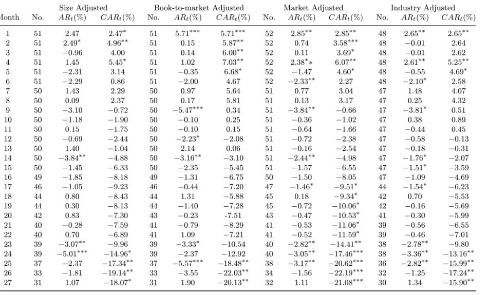
Table 2 presents the size-, BM-, market-, and industry-adjusted aver-age returns and CARs over the 36 months following the placements. The benchmark-adjusted returns are positive in the first few months after the is-sue. For the size-adjusted and the market-adjusted returns series, the CARs

(8)

No v em b er 26, 2002 11:18 WS P C /155-R P BFMP 00076 424 • She ng -Sy a n C h e n e t a l.

Table 2. Long-run Abnormal Returns Following Private Placements

Size Adjusted Book-to-market Adjusted Market Adjusted Industry Adjusted Month No. ARt(%) CARt(%) No. ARt(%) CARt(%) No. ARt(%) CARt(%) No. ARt(%) CARt(%)

1 51 2.47 2.47∗ 51 5.71∗∗∗ 5.71∗∗∗ 52 2.85∗∗ 2.85∗∗ 48 2.65∗∗ 2.65∗∗ 2 51 2.49∗ 4.96∗∗ 51 0.15 5.87∗∗ 52 0.74 3.58∗∗∗ 48 −0.01 2.64 3 51 −0.96 4.00 51 0.14 6.00∗∗ 52 0.11 3.69∗ 48 −0.01 2.62 4 51 1.45 5.45∗ 51 1.02 7.03∗∗ 52 2.38∗∗ 6.07∗∗ 48 2.61∗∗ 5.25∗∗ 5 51 −2.31 3.14 51 −0.35 6.68∗ 52 −1.47 4.60∗ 48 −0.55 4.69∗ 6 51 −2.29 0.86 51 −2.00 4.67 52 −2.33∗∗ 2.27 48 −2.10∗ 2.58 7 50 1.43 2.29 50 0.97 5.64 51 0.77 3.04 47 1.48 4.07 8 50 0.09 2.37 50 0.17 5.81 51 0.13 3.17 47 0.25 4.32 9 50 −3.10 −0.72 50 −5.47∗∗∗ 0.34 51 −3.84∗∗ −0.66 47 −3.81∗ 0.51 10 50 −1.18 −1.90 50 −0.10 0.25 51 −0.36 −1.02 47 0.38 0.89 11 50 0.15 −1.75 50 −0.10 0.15 51 −0.64 −1.66 47 −0.44 0.45 12 50 −0.69 −2.44 50 −2.23∗ −2.08 51 −0.72 −2.38 47 −0.58 −0.13 13 50 1.40 −1.04 50 2.14 0.06 51 −0.16 −2.54 47 −0.18 −0.31 14 50 −3.84∗∗ −4.88 50 −3.16∗∗ −3.10 51 −2.44∗∗ −4.98 47 −1.76∗ −2.07 15 50 −1.45 −6.33 50 −2.35 −5.45 51 −1.57 −6.55 47 −1.51∗ −3.59 16 49 −1.85 −8.18 49 −1.31 −6.75 50 −1.50 −8.05 47 −1.09 −4.69 17 46 −1.05 −9.23 46 −0.44 −7.20 47 −1.46∗ −9.51∗ 44 −1.54∗ −6.23 18 44 0.80 −8.43 44 1.31 −5.88 45 0.18 −9.34∗ 42 0.70 −5.53 19 44 0.30 −8.13 44 −1.40 −7.28 45 −0.72 −10.06∗ 42 −0.16 −5.69 20 42 0.83 −7.30 43 −0.23 -7.51 43 −0.47 −10.53∗ 41 −0.30 −5.99 21 40 −0.28 −7.59 41 −0.79 −8.29 41 −0.53 −11.06∗ 39 −0.56 −6.55 22 40 0.70 −6.89 41 1.09 −7.21 41 −0.52 −11.59∗ 39 −0.46 −7.01 23 39 −3.07∗∗ −9.96 39 −3.33∗ −10.54 40 −2.82∗∗ −14.41∗∗ 38 −2.78∗∗ −9.80 24 39 −5.01∗∗∗ −14.96∗ 39 −2.37 −12.92 40 −3.05∗∗ −17.46∗∗∗ 38 −3.36∗∗ −13.16∗∗ 25 37 −2.37 −17.34∗∗ 37 −5.57∗∗∗ −18.48∗∗ 38 −3.17∗∗ −20.62∗∗∗ 36 −2.82∗∗ −15.99∗∗ 26 33 −1.81 −19.14∗∗ 33 −3.55 −22.03∗∗ 34 −1.56 −22.19∗∗∗ 32 −1.25 −17.24∗∗ 27 31 1.07 −18.07∗ 31 1.90 −20.13∗∗ 32 1.11 −21.08∗∗∗ 30 1.34 −15.90∗∗

(9)

No v em b er 26, 2002 11:18 WS P C /155-R P BFMP 00076 Lo ng-r un Sto c k P erf o rmance o f E q u ity-I ssuing F irms • 425

Table 2. (continued) Long-run Abnormal Returns Following Private Placements

Size Adjusted Book-to-market Adjusted Market Adjusted Industry Adjusted Month No. ARt(%) CARt(%) No. ARt(%) CARt(%) No. ARt(%) CARt(%) No. ARt(%) CARt(%)

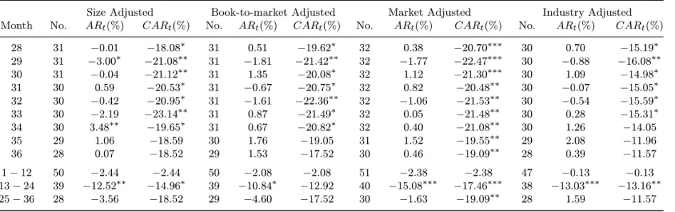
28 31 −0.01 −18.08∗ 31 0.51 −19.62∗ 32 0.38 −20.70∗∗∗ 30 0.70 −15.19∗ 29 31 −3.00∗ −21.08∗∗ 31 −1.81 −21.42∗∗ 32 −1.77 −22.47∗∗∗ 30 −0.88 −16.08∗∗ 30 31 −0.04 −21.12∗∗ 31 1.35 −20.08∗ 32 1.12 −21.30∗∗∗ 30 1.09 −14.98∗ 31 30 0.59 −20.53∗ 31 −0.67 −20.75∗ 32 0.82 −20.48∗∗ 30 −0.07 −15.05∗ 32 30 −0.42 −20.95∗ 31 −1.61 −22.36∗∗ 32 −1.06 −21.53∗∗ 30 −0.54 −15.59∗ 33 30 −2.19 −23.14∗∗ 31 0.87 −21.49∗ 32 0.05 −21.48∗∗ 30 0.28 −15.31∗ 34 30 3.48∗∗ −19.65∗ 31 0.67 −20.82∗ 32 0.40 −21.08∗∗ 30 1.26 −14.05 35 29 1.06 −18.59 30 1.76 −19.05 31 1.52 −19.55∗∗ 29 2.08 −11.96 36 28 0.07 −18.52 29 1.53 −17.52 30 0.46 −19.09∗∗ 28 0.39 −11.57 1− 12 50 −2.44 −2.44 50 −2.08 −2.08 51 −2.38 −2.38 47 −0.13 −0.13 13− 24 39 −12.52∗∗ −14.96∗ 39 −10.84∗ −12.92 40 −15.08∗∗∗ −17.46∗∗∗ 38 −13.03∗∗∗ −13.16∗∗ 25− 36 28 −3.56 −18.52 29 −4.60 −17.52 30 −1.63 −19.09∗∗ 28 1.59 −11.57 Note:

This table presents the average monthly adjusted returns (ARt) and cumulative average adjusted returns (CARt) expressed as percentages

for the 36 months following the private placement. ARtis computed as the arithmetic average of the amounts by which the issuing firm’s

returns exceed the matched firm’s returns (for the size-adjusted returns and the book-to-market adjusted returns) or the SES All Share Index returns (for the market adjusted returns) or the industry sector returns (for the industry adjusted returns). The industry sector comparison is undertaken because the size of the Stock Exchange of Singapore precludes effective simultaneous matching on the basis of size and industry. The t-statistic for the average adjusted return is computed each month as ARt√nt/sdt where nt is the number

of observations in month t and sdtis the cross-sectional standard deviation of the adjusted returns for month t. The t-statistic for the

cumulative average adjusted return to month t is computed as CARt√nt/csdt where csdt = [t· var + 2 · (t − 1) · cov]1/2, var is the

average (over 36 months) cross-sectional variance, and cov is the first order autocovariance of the ARtseries. The var values for the size-,

book-to-market-, market-, and industry-adjusted returns are 0.01102, 0.00116, 0.00661, and 0.00641 respectively. The cov values for the size-, book-to-market-, market-, and industry-adjusted returns are 6.03× 10−5, 4.39× 10−5, 6.28× 10−5, and 6.01× 10−5 respectively. “∗∗∗”, “∗∗”, and “∗” denote two-tailed significance at the 1%, 5%, and 10% levels, respectively.

(10)

are negative in each month after month nine for the remaining 27 months. For the BM-adjusted and industry-adjusted returns series, the CARs are negative from around month 12.14

The results on the yearly average adjusted returns show that the un-derperformance occurs mainly in the second year. The two-year post-issue CARs range from−12.9 percent to −17.5 percent depending on the bench-mark used, while the three-year post-issue CARs range from−11.6 percent to −19.1 percent. Because of data limitation, the three-year stock returns are seriously truncated, and hence the sample size for the three-year returns is small. Hence, we focus on the two-year returns in our subsequent analysis. Table 3 shows the distribution of the two-year holding period returns for the sample firms and control firms.15 The underperformance of the issuing firms is evident in almost all quartiles. The issuing firms underperform the control firms by between 15.5 percent and 18.5 percent on average. Both the mean and median difference in holding period returns between sample firms and control firms are statistically significant at conventional levels. The wealth relatives are all below one and the fractions underperforming are statistically different from 0.5 at conventional levels.

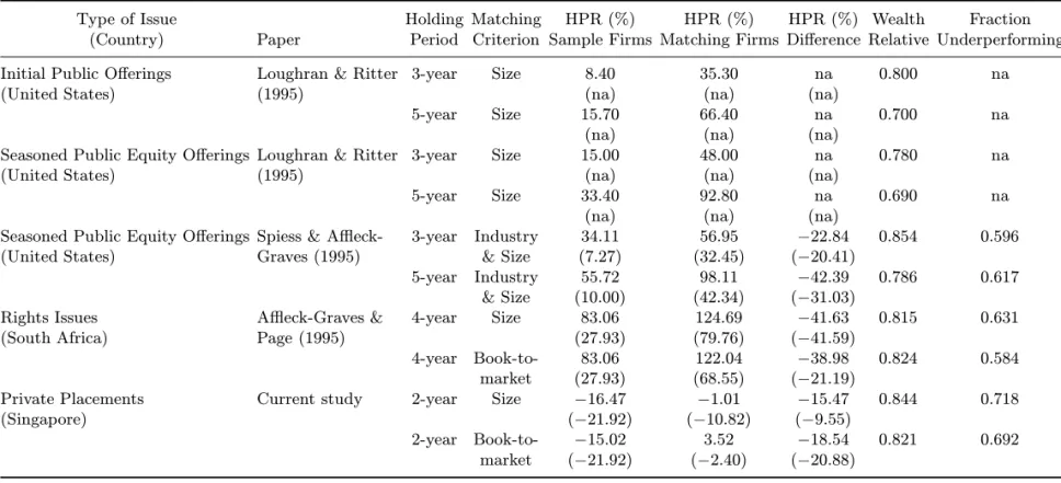
Table 4 shows a comparison of our results with those in previous studies on long-run stock underperformance of equity-issuing firms. For ease of pre-sentation, only the results of selected benchmarks are presented. Note that the average holding period return for the sample firms is negative, whereas those for existing studies are positive. The wealth relatives for the Singapore sample firms are similar to those found in other studies on IPOs, SEOs, and rights issues.

4. Analysis of Post-Issue Stock Performance

This section presents the results of our univariate and cross-sectional analysis of the post-issue performance of the sample firms, as well as the examination of earnings management surrounding the year of issue. Table 5 presents the univariate results using size-adjusted returns. Though not reported, results based on book-to-market adjusted returns are qualitatively similar.

14

One possible reason for the underperformance to start several months after the private placements is that the purchasers may have given some undertaking not to immediately resell the placement shares. However, this undertaking, if any, is not publicly observable.

15_{For brevity, Table 3 shows only the results using the size and the book-to-market}

(11)

Long-run Stock Performance of Equity-Issuing Firms• 427 Table 3. Two-year Holding Period Returns, Wealth Relative, and Fraction Underper-forming Following Private Placements

Two-year Holding Period Returns (%)

Fraction

Sample Wealth

Under-Firms Benchmark Difference Relative Performing Panel A: Size Adjusted

Minimum −75.31 −55.22 −96.54 First Quartile −33.93 −23.94 −29.33 Median −21.92 −10.82 −9.55∗∗ Third Quartile 11.06 13.23 2.26 Maximum 68.56 81.78 57.22 Mean −16.47 −1.01 −15.47∗∗ 0.844 0.718∗∗

Panel B: Book-to-market Adjusted

Minimum −75.31 −46.89 −163.41 First Quartile −33.93 −19.46 −39.82 Median −21.92 −2.40 −20.88∗∗ Third Quartile 11.06 17.85 11.20 Maximum 69.69 181.83 89.37 Mean −15.02 3.52 −18.54∗ 0.821 0.692∗ Note:

Average holding period returns are computed as_N1 PN_i=1hQT_t=1(1 + rit)− 1

i

, where N = 39 (the number of firms); Rit is the return on stock i for month t following private

placement; and Ti= 24 (the number of months from the placement announcement date).

If the original matched firm delists or itself has a private placement, a second and possibly third matched firm is spliced into the matched firm return series. The wealth relative is defined as the ratio of one plus the average holding period return for the issue firms to one plus the average holding period return for the matched firms. The significance of the mean and median difference in holding period returns are tested using the standard t-test and the Wilcoxon signed rank test, respectively. The significance of the fraction underperforming is tested using the non-parametric test of proportion, zcalc = (p− π)/(π(1 − π)/N)0.5,

where p = the proportion of times the matched firm return exceeds the issue firm return, and π = 0.5. “∗∗” and “∗” denote significance at the 1% and 5% level respectively, using two-tailed tests.

Panel A, Table 5, shows the results by partitioning the sample into small and large firms. Small firms are those with market capitalization less than the sample median while large firms are those with market capitalization greater than the sample median. While both small and large issuing firms underperform the comparison firms, small firms show a greater degree of un-derperformance than large firms. The results are consistent with the notion that smaller firms, which have a greater degree of information asymmetry, are more likely to take advantage of windows of opportunity to issue equity

(12)

No v em b er 26, 2002 11:18 WS P C /155-R P BFMP 00076

Table 4. A Comparison of Long-run Stock Performance of Firms Conducting Equity Issues

Type of Issue Holding Matching HPR (%) HPR (%) HPR (%) Wealth Fraction (Country) Paper Period Criterion Sample Firms Matching Firms Difference Relative Underperforming Initial Public Offerings Loughran & Ritter 3-year Size 8.40 35.30 na 0.800 na

(United States) (1995) (na) (na) (na)

5-year Size 15.70 66.40 na 0.700 na (na) (na) (na)

Seasoned Public Equity Offerings Loughran & Ritter 3-year Size 15.00 48.00 na 0.780 na

(United States) (1995) (na) (na) (na)

5-year Size 33.40 92.80 na 0.690 na (na) (na) (na)

Seasoned Public Equity Offerings Spiess & Affleck- 3-year Industry 34.11 56.95 −22.84 0.854 0.596 (United States) Graves (1995) & Size (7.27) (32.45) (−20.41)

5-year Industry 55.72 98.11 −42.39 0.786 0.617 & Size (10.00) (42.34) (−31.03)

Rights Issues Affleck-Graves & 4-year Size 83.06 124.69 −41.63 0.815 0.631 (South Africa) Page (1995) (27.93) (79.76) (−41.59)

4-year Book-to- 83.06 122.04 −38.98 0.824 0.584 market (27.93) (68.55) (−21.19)

Private Placements Current study 2-year Size −16.47 −1.01 −15.47 0.844 0.718

(Singapore) (−21.92) (−10.82) (−9.55)

2-year Book-to- −15.02 3.52 −18.54 0.821 0.692 market (−21.92) (−2.40) (−20.88)

Notes:

This table presents a comparison of long-run stock underperformance of equity issues based on selected results in recent papers and the present study. Median values are shown in parentheses below mean values. na denotes “not available”.

(13)

Long-run Stock Performance of Equity-Issuing Firms• 429 Table 5. Univariate Analysis of Two-year Holding Period Returns, Wealth Relative, and Fraction Underperforming

HPR (%) Fraction

HPR (%) Size-matched Wealth

Under-No. Sample Firms Benchmark Relative performing Panel A: Analysis by Firm Size

Small Firms 19 −33.16 −9.10 0.735 0.882∗∗

(−30.25) (−10.82)

Large Firms 20 −3.58 5.25 0.916 0.591

(−17.10) (−10.11) Panel B: Analysis by Book-to-market

Low BM Firms 19 −7.51 0.31 0.922 0.714∗

(−19.00) (−15.89)

High BM Firms 20 −26.93 −2.54 0.750 0.722

(−26.79) (−6.86)

Panel C: Analysis by Years Since Listing

≤ 5 9 −9.06 −7.59 0.984 0.556

(−15.54) (−17.80)

> 5 30 −18.70 0.97 0.805 0.767∗∗

(−24.53) (−5.12) Note:

Average holding period returns are computed as _N1 PN_i=1hQt_t=1(1 + Rit)− 1

i , where N = 39 (the number of firms); Ritis the return on stock i for month t following private

placement; and Ti= 24 (the number of months from the placement announcement date).

If the original matched firm delists or itself has a private placement, a second and possibly third matched firm is spliced into the matched firm return series. The wealth relative is defined as the ratio of one plus the average holding period return for the issue firms to one plus the average holding period return for the matched firms. Small firms are those with market capitalization less than the sample median while large firms are those with market capitalization greater than the sample median. Market capitalization is measured as at December 31 prior to the private placement. Low BM firms are those with book-to-market ratio less than the sample median while high BM firms are those with BM ratio greater than the sample median. BM ratio is computed as the firm’s book value of equity divided by its market value of equity at the fiscal year end prior to the private placement. Median values are in parentheses below mean values. The significance of the fraction underperforming is tested using the non-parametric test of proportion, zcalc =

(p− π)/(π(1 − π)/N)0.5, where p = the proportion of times the matched firm return exceeds the issue firm return, and π = 0.5. “∗∗” and “∗” denote significance at the 1% and 5% level respectively, using two-tailed tests. na denotes “not available”.

when they are overvalued (Affleck-Graves and Page, 1995; Loughran and Ritter, 1995; and Spiess and Affleck-Graves, 1995).

In Panel B, Table 5, the sample is partitioned by the BM ratio. Low-BM firms are those with BM less than the sample median while high-BM firms are those with BM greater than the sample median. The underperformance

(14)

is evident in both groups. The results show that low-BM firms tend to under-perform less than high-BM firms. Since the BM ratio is a proxy for growth opportunities,16 _{our evidence supports the notion that firms with poorer}

growth opportunities are more likely to time to issue equity when they are overvalued.

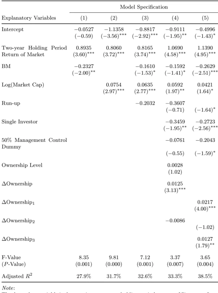
In Panel C, Table 5, the sample is sub-divided into firms that have been listed for less than or equal to five years prior to the placement and those which have been listed for longer than five years. This partitioning is similar to that used in Loughran and Ritter (1995). The results show that there is no clear evidence that younger firms underperform more than older firms.17 In the cross-sectional regressions of the two-year holding period returns, we include the explanatory variables as described in Table 6. The specifica-tion models and results are reported in Table 7.18 The matching two-year holding period return of the market index is included in all regression mod-els to control for market-wide effects. T -values are computed using White (1980)-corrected standard errors.

As shown in Table 7, the explanatory power of book-to-market and firm size is tested separately in Models 1 and 2, respectively, and jointly in Model 3. In Model 4, ownership and other variables are included. Runup, as mea-sured by the cumulative abnormal returns from days −59 to −2 using the market model estimated from days −200 to −60, is included to control for any mean reversion in returns. The single investor dummy, which equals one if placement shares are sold to one buyer and zero elsewhere, is to assess the monitoring effect of a single investor.19 The 50 percent management control dummy, which equals 1 if management holdings fall below 50 percent after the issue and zero elsewhere, is included to check whether a dilution by insid-ers to below 50 percent have any long-run negative impact on stock prices.20

16

See, for example, Hertzel and Smith (1993) and Barclay and Smith (1995a and 1995b). High-BM stocks are sometimes called value stocks while low-BM stocks are called glamour stock. Fama and French (1992) and Lakonishok, Shleifer, and Vishny (1994) find that value stocks outperform glamour stocks in the US after controlling for differences in size. Results in this study suggest that the glamour stocks outperform the value stocks. Desai and Jain (1997) find similar results in their stock splits sample.

17_{We have also examined the stock performance by year of placements and find no evidence}

suggesting that the long-run underperformance is concentrated in a particular year.

18

Our results are similar when we use two-year market-adjusted holding period returns as the dependent variable.

19

See Shleifer and Vishny (1986) and others.

20_{Holderness and Sheehan (1988) find a negative announcement-period return in the case}

of a majority-block trade. A placement in which management reduce their holding to below 50% (for example, from 55% to 45%) is, to a certain extent, the reverse of a majority-block trade, which would suggest a negative market reaction. Also, the fact that management

(15)

Long-run Stock Performance of Equity-Issuing Firms• 431 Table 6. Description of Explanatory Variables

Explanatory Variables Description Two-year Holding Period

Return of Market

Holding period return of the value-weighted Stock Exchange of Singapore All-Share Index for the 24 months from the announcement date.

BM Book-to-market ratio as measured by the firm’s book value of equity divided by its market value of equity at the fiscal year end prior to the placement.

Log(Market Cap) Log of market capitalization at December 31 prior to the announcement date.

Run-up Cumulative abnormal returns from days−59 to −2 using market model estimated from days−200 to −60.

Single Investor A dummy variable that equals 1 if placement shares are sold to a single buyer and 0 elsewhere.

50% Management Control Dummy

A dummy variable that equals 1 if management holdings fall below 50% after the issue and 0 elsewhere.

Ownership Level Ownership concentration level (total holdings of directors and 5% blockholders).

∆Ownership Changes in total holdings of directors and 5blockholders (total holdings after minus total holdings before the place-ment).

∆Ownership1, ∆Ownership2, ∆Ownership3

Piecewise regression variables for ?Ownership whereby the total change in ownership is split into the portion mov-ing the ownership level between 0% and 50%, 50% and 75%, and 75% and greater, respectively (see Wruck, 1989, for a description of piecewise regression using ownership concentration).

Ownership level and ∆ownership, defined as total holdings and changes in total holdings of directors and blockholders respectively, are included to assess the impact of ownership variables on the long-run returns.21 Model 5 is a piecewise regression where the ∆ownership variable splits the total

are willing to lose 50% control is a signal that they are “cashing out”.

21

These definitions are the same as those in Wruck (1989). We have also tested the signifi-cance of issue price discount, fraction placed and a dummy variable that equals 1 if the year of placement is 1993, the year in which there was the highest number of private placements in our sample, and zero otherwise. None of these variables is significant. Further, we have tested the capital expenditure variables in Cheng (1994) and Loughran and Ritter (1997) and find that the variables have no explanatory power. Cheng’s (1994) capital expendi-ture variable is measured as CHGCAP Xt= (CAP Xt+CAP Xt+1_{2P RCDS})−(CAP X_t t−1+CAP Xt−2),

where t is the fiscal year in which the issue is done; CAP X is capital expenditures; and PRCDS is the issue size. Loughran and Ritter’s (1997) capital expenditure measure is the change in capital expenditures from fiscal year−1 to 0 expressed as a percentage of assets at the end of year−1.

(16)

Table 7. Cross-sectional Regressions of the Two-year Holding Period Returns

Model Specification

Explanatory Variables (1) (2) (3) (4) (5)

Intercept −0.0527 −1.1358 −0.8817 −0.9111 −0.4996

(−0.59) (−3.56)∗∗∗ _(−2.92)∗∗∗ _(−1.95)∗∗ _(−1.43)∗

Two-year Holding Period Return of Market 0.8935 0.8060 0.8165 1.0690 1.1390 (3.60)∗∗∗ (3.72)∗∗∗ (3.74)∗∗∗ (4.58)∗∗∗ (4.95)∗∗∗ BM −0.2327 −0.1610 −0.1592 −0.2629 (−2.00)∗∗ (−1.53)∗ (−1.41)∗ (−2.51)∗∗∗ Log(Market Cap) 0.0754 0.0635 0.0592 0.0421 (2.97)∗∗∗ (2.77)∗∗∗ (1.97)∗∗ (1.64)∗ Run-up −0.2032 −0.3607 (−0.71) (−1.64)∗ Single Investor −0.3459 −0.2723 (−1.95)∗∗ (−2.56)∗∗∗ 50% Management Control Dummy −0.0761 −0.2043 (−0.55) (−1.59)∗ Ownership Level 0.0028 (1.02) ∆Ownership 0.0125 (3.13)∗∗∗ ∆Ownership1 0.0217 (4.00)∗∗∗ ∆Ownership2 −0.0086 (−1.02) ∆Ownership3 0.0127 (1.79)∗∗ F-Value 8.35 9.81 7.12 3.37 3.65 (P -Value) (0.001) (0.000) (0.001) (0.007) (0.004) Adjusted R2 27.9% 31.7% 32.6% 33.3% 38.5% Note:

The dependent variable is the post-issue two-year holding period returns of Singapore firms that have conducted private placements from 1988–1993. See Table 6 for description of the explanatory variables. The number of observations is 39. T -values based on White (1980)-corrected standard errors are in parentheses. “∗∗∗”, “∗∗” and “∗” denote significance (using a one-tailed test) at the 1% , 5% , and 10% levels, respectively.

(17)

change in ownership into the portion moving the ownership level between zero percent and 50 percent, 50 percent and 75 percent, and 75 percent and greater.22

The results show that the coefficient on BM is negative and significant at conventional levels. Thus, firms with higher BM perform poorer than firms with lower BM. The coefficient on the firm size variable is positive and significant, suggesting that smaller firms underperform more. The results on BM and firm size are consistent with those in the univariate analysis.

The coefficient on the run-up variable is negative but it is significant at the 10 percent level only in Model 5. The coefficient on the single investor dummy is negative and is significant, suggesting that any positive monitoring effect of a single investor is not evident in the long run. The coefficient on the 50 percent management control dummy is negative but it is significant only at 10 percent level in Model 5. Nevertheless, the negative sign indicates that firms in which management dilute their holdings to below 50 percent perform poorly in the long run.

In Model 4, the coefficient on the ownership level variable is not signifi-cant whereas the coefficient on ∆ownership is signifisignifi-cantly positive. This sug-gests that the greater the reduction in ownership concentration the poorer the long-run stock performance. This evidence is consistent with Jensen and Meckling’s (1976) alignment-of-interests hypothesis.23The result is also consistent with the management-timing hypothesis as managers are likely to place out more shares to outsiders when their firm’s equity is overval-ued. The piecewise regression in Model 5 shows that the positive relation between ownership concentration and holding period return of sample firms is significant only for an ownership concentration level below 50 percent and above 75 percent, suggesting that the relation may be nonlinear.

Previous studies also show that the long-run stock underperformance may be due to the market’s inability to fully incorporate the effects of earnings management surrounding equity issues. To check whether there is

22_{This study cannot use the same turning points (5% and 25%) as in Wruck (1989) because}

there are only two firms in the sample with ownership concentration less than 25%. We have also tried different combinations of turning points [(45%, 70%), (45%, 75%), (50%, 70%), (50%, 80%), and (60qualitatively similar results. The first quartile, median and third quartile of the ownership concentration in the sample are 46.4%, 60.5%, and 72.9%, respectively.

23

Traditionally, Jensen and Meckling’s alignment-of-interests hypothesis is tested using announcement-period returns. However, it is possible that the alignment-of-interests effect may take some time to be fully reflected in the stock price.

(18)

significant earnings management surrounding the year of placement in our sample firms, we use the modified Jones (1991) model of expected accruals as follows:24

T Ait/Ait−1= αi[1/Ait−1] + β1i[(∆REVit− ∆RECit)/Ait−1]

+ β2i[P P Eit−1/Ait−1] + εit,

where T Ait= total accruals in year t for firm i;25∆REVit= revenuetminus

revenuet−1 for firm i; ∆RECit = receivablestminus receivablest−1 for firm i;

P P Eit−1 = gross property, plant, and equipment at the end of year t− 1 for

firm i; Ait−1 = total assets at the end of year t− 1 for firm i; and εit= an

error term. This study uses as many years as are available excluding years −1, 0, and +1 as the estimation period.26 _{Discretionary accruals for years}

−1, 0, and +1 are calculated as:

Uip= T Aip/Aip−1− {ai[1/Aip−1] + b1i[(∆REVip− ∆RECip)/Aip−1]

+ b2i[P P Eip−1/Aip−1]} ,

where Uip= discretionary accruals for firm i in year p(p =−1, 0, and + 1);

ai, b1i, and b2i= estimated coefficients for expected accruals for firm i.

Following Jones (1991) and others, the standardized prediction errors are computed as Vip = Uip/ˆσ(uip), where Uip is the discretionary accrual

for firm i in prediction year p as defined above, and ˆσ(uip) is the estimated

standard deviation of the abnormal accruals in the prediction periods. The Vips are aggregated across the firms into a Z-statistic, ZVp=

ΣNi=1Vip

h ΣN

i=1(Ti−3)_(Ti−5)

i1/2,

where Ti is the number of observations in the estimation period for firm i. 24

Dechow, Sloan, and Sweeney (1995) find that the modified Jones (1991) model has more power in detecting earnings management than the Healy (1985) model, the DeAngelo (1986) model, the Jones (1991) model, and the industry model. Teoh, Welch, and Wong (1998b) use the industry model. There is no similar study in Singapore to test the relative power of various accruals-based models for detecting earnings management. We use the modified Jones (1991) model because it incorporates the economic activities of the firm during the test period.

25

Following Healy (1985), Jones (1991) and others, we measure total accruals as T At=

(∆CAt− ∆Casht)− (∆CLt− ∆ST Dt)− Depnt, where ∆CA = change in current

as-sets; ∆Cash = change in cash and cash equivalents; ∆CL = change in current liabilities; ∆ST D = change in debt included in current liabilities; and Depnt = depreciation and

amortization expense.

26

The number of observations for each firm in the regression ranges from 4 to 19 (with a mean of 10.4 and a median of 9 years). Firms with fewer than four observations are excluded. The final sample of firms for the test for earnings management is 51.

(19)

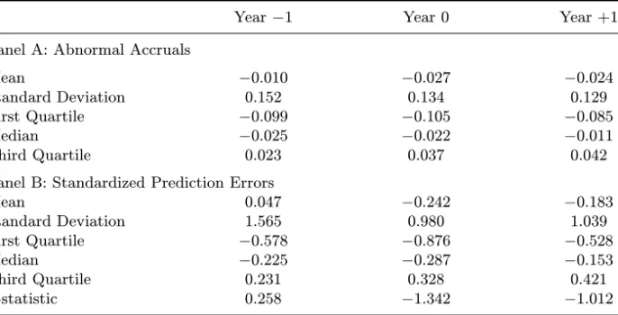
Long-run Stock Performance of Equity-Issuing Firms• 435 Table 8. Abnormal Accruals and Standardized Prediction Errors for Firms Conducting Private Placements During 1988–1993

Year−1 Year 0 Year +1

Panel A: Abnormal Accruals

Mean −0.010 −0.027 −0.024

Standard Deviation 0.152 0.134 0.129

First Quartile −0.099 −0.105 −0.085

Median −0.025 −0.022 −0.011

Third Quartile 0.023 0.037 0.042

Panel B: Standardized Prediction Errors

Mean 0.047 −0.242 −0.183 Standard Deviation 1.565 0.980 1.039 First Quartile −0.578 −0.876 −0.528 Median −0.225 −0.287 −0.153 Third Quartile 0.231 0.328 0.421 Z-statistic 0.258 −1.342 −1.012 Note:

Abnormal accruals are defined as the difference between the actual and expected ac-cruals. The expected accruals model is: T Ait/Ait−1 = αi[1/Ait−1] + β1i[(∆REVit−

∆RECit)/Ait₋₁] + β2i[P P Eit₋₁/Ait₋₁] + εit, where T Ait is the total accruals in year

t for firm i; ∆REVitis the annual change in revenue for firm i; ∆RECit is the annual

change in receivables for firm i; P P Eit₋₁ is the gross property, plant, and equipment at

the end of year t− 1 for firm i; Ait−1 is the total assets at the end of year t− 1 for

firm i; and εit is an error term. Coefficients for each of the sample firms are estimated

over all years excluding years −1, 0, and 1 for which data are available. Year 0 is the year of announcement. Because of data limitation, the sample consists of 51 private place-ments during the 1988-1993 period. Standardized prediction errors (Vip’s) are defined as:

Vip= AAip/σ(AAip), where AAipis the abnormal accrual for firm i in prediction year p as

defined above; and σ(AAip) is the estimated standard deviation of the abnormal accruals

in the prediction periods. The Z-statistic aggregates the 51 standardized prediction errors (Vip0s) in each period using the central limit theorem: Z = ΣVip/[Σ(Ti− 3)/(Ti− 5)]0.5.

Tiis the number of observations in the estimation period for firm i.

Table 8 shows the discretionary accruals, standardized prediction errors, and the Z-statistics. The Z-statistics are not significant at conventional lev-els. Thus, we find no evidence of significant earnings management surround-ing the year of issue. This may be explained by the fact that nine out of 10 firms in the sample are audited by reputable international accounting firms, which may provide effective monitoring on managerial behavior with respect to discretionary accruals, especially those that would increase reported earn-ings. Further, DeFond and Park (1997) show that when current earnings are good and expected future earnings are poor,27 managers have incentive to

27

(20)

make income-decreasing discretionary accruals. This incentive may cancel out the incentive to make income-increasing discretionary accruals to ob-tain a better placement price. Finally, our insignificant results may be due to the small sample size available for our study.

5. Concluding Remarks

We find that Singapore listed firms which have conducted private placements exhibit long-run stock underperformance similar to those reported for IPOs, SEOs and rights issues. We find that the stock underperformance is posi-tively related to firm size and negaposi-tively related to book-to-market ratio. Our evidence is consistent with the timing hypothesis because smaller firms and firms with poorer growth opportunities may have greater incentive to issue shares when they are overvalued. We also find a significant positive relation between long-run stock performance and change in ownership concentration. This is consistent with the alignment-of-interests hypothesis. Finally, we do not find evidence supporting the earnings-management hypothesis.

References

Affleck-Graves, J. and M. J. Page (1995), “The Timing and Subsequent Performance of Seasoned Offerings: The Case of Rights Issues”, Working Paper, University of Notre Dame and University of Cape Town.

Aggarwal, R., R. Leal, and L. Hernandez (1993), “The Aftermarket Performance of Initial Public Offerings in Latin America”, Financial Management 22, 42–53. Alli, K. L. and D.J. Thompson (1993), “The Wealth Effects of Private Stock

Place-ments Under Regulation D”, Financial Review 28, 329–350.

Barclay, M. J. and C. W. Smith, Jr. (1995a), “The Maturity Structure of Corporate Debt”, Journal of Finance 50, 609–631.

Barclay, M. J. and C. W. Smith, Jr. (1995b), “The Priority Structure of Corporate Liabilities”, Journal of Finance 50, 899–917.

Cheng, L. -L. (1994), “Equity Issue Underperformance and the Timing of Security Issues”, Working Paper, Massachusetts Institute of Technology.

DeAngelo, L. (1986), “Accounting Numbers as Market Valuation Substitutes: A Study of Management Buyouts of Public Stockholders”, The Accounting Review 41, 400–420.

Dechow, P. M., R. G. Sloan, and A. P. Sweeney (1995), “Detecting Earnings Man-agement”, The Accounting Review 70, 193–225.

DeFond, M. L. and C. W. Park (1997), “Smoothing Income in Anticipation of Future Earnings”, Journal of Accounting and Economics 23, 115–139.

Desai, H. and P. C. Jain (1997), “Long-run Common Stock Returns Following Stock Splits and Reverse Splits”, Journal of Business 70, 409–433.

Fama, E. F. and K. R. French (1992), “The Cross-section of Expected Stock Re-turns”, Journal of Finance 47, 427–465.

(21)

Long-run Stock Performance of Equity-Issuing Firms• 437 Healy, P. M. (1985), “The Effect of Bonus Schemes on Accounting Decisions”,

Journal of Accounting and Economics 7, 85–107.

Hertzel, M. and R. L. Smith (1993), “Market Discounts and Shareholder Gains for Placing Equity Privately”, Journal of Finance 48, 459–485.

Ho, K. W., S. S. Chen, C. F. Lee, and G. H. H. Yeo (2000), “Wealth Effects of Private Equity Placements: Evidence from Singapore”, Working Paper, Rutgers University.

Holderness, C. G. and D. P. Sheehan (1988), “The Role of Majority Shareholders in Publicly Held Corporations”, Journal of Financial Economics 20, 317–346. Jensen, M. C. and W. H. Meckling (1976), “Theory of the Firm: Managerial

Be-havior, Agency Costs, and Capital Structure”, Journal of Financial Economics 3, 305–360.

Jones, J. (1991), “Earnings Management During Import Relief Investigations”, Journal of Accounting Research 29, 193–228.

Lakonishok, J., A. Shleifer, and R. W. Vishny (1994), “Contrarian Investing, Ex-trapolation and Risk”, Journal of Finance 49, 1541–1578.

Levis, M. (1993a), “The Long-run Performance of Initial Public Offerings: The UK Experience 1980–1988”, Financial Management 22, 28–41.

Levis, M (1993b), “Initial Public Offerings, Subsequent Rights Issues and Long-run Performance”, Working Paper, City University, London.

Loughran, T. and J. R. Ritter (1995), “The New Issue Puzzle”, Journal of Finance 50, 23–51.

Loughran, T. and J. R. Ritter (1997), “The Operating Performance of Firms Con-ducting Seasoned Equity Offerings”, Journal of Finance 52, 1823–1850. Loughran, T., J. R. Ritter, and K. Rydqvist (1994), “Initial Public Offerings:

In-ternational Insights”, Pacific-Basin Finance Journal 2, 165–199.

Ritter, J. R. (1991), “The Long-run Performance of Initial Public Offerings”, Jour-nal of Finance, 46, 3–27.

Shleifer, A. and R. W. Vishny (1986), “Large Shareholders and Corporate Control”, Journal of Political Economy 94, 461–488.

Spiess, D. K. and J. Affleck-Graves (1995), “Underperformance in Long-run Stock Returns Following Seasoned Equity Offerings”, Journal of Financial Economics 38, 243–267.

Teoh, S. H., I. Welch, and T. J. Wong (1998a), “Earnings Management and the Long-run Market Performance of Initial Public Offerings”, Journal of Finance 53, 1935–1974.

Teoh, S. H., I. Welch, and T. J. Wong (1998b), “Earnings Management and the Un-derperformance of Seasoned Equity Offerings”, Journal of Financial Economics 50, 63–99.

White, H. (1980), “A Heteroskedasticity-consistent Covariance Matrix Estimator and a Direct Test for Heteroskedasticity”, Econometrica 48, 817–838.

Wong, K. A. (1989), “The Firm Size Effect on Stock Returns in a Developing Stock Market”, Economics Letters 30, 61–65.

Wong, K. A. and M. S. Lye (1990), “Market Values, Earnings’ Yields and Stock Returns”, Journal of Banking and Finance 14, 311–326.

(22)

Wong, K. A. and C. L. Tan (1992), “The Price to Book Value Effect on Stock Returns in Singapore”, Securities Industry Review 18, 15–22.

Wruck, K. H. (1989), “Equity Ownership Concentration and Firm Value: Evidence from Private Equity Financings”, Journal of Financial Economics 23, 3–28.