藉由粒線體相關疾病之基因型及表徵型的網路分析來預測疾病基因
32
0
0
全文
(2) 藉由粒線體相關疾病之基因型及表徵型的網路 分析來預測疾病基因. Predict Candidate Genes by Network Analysis of Genotypes and Phenotypes for Mitochondrion Diseases. 研 究 生:陳俊睿. Student:Chun-Jui Chen. 指導教授:盧鴻興. Advisor: Henry Horng-Shing Lu. 國 立 交 通 大 學 統計學研究所 碩 士 論 文 A Thesis Submitted to Institute of Statistics College of Science National Chiao Tung University in Partial Fulfillment of the Requirements for the Degree of Master in Statistics June 2007. Hsinchu, Taiwan, Republic of China 中華民國九十六年六月.
(3) 藉由粒線體相關疾病之基因型及表徵型的網路 分析來預測疾病基因. 研究生:陳俊睿. 指導教授:盧鴻興 博士. 國立交通大學統計學研究所. 摘要 在遺傳疾病的研究上,基因與疾病之間的關係是我們感興趣的。 其中我們更感興趣的是,是否仍有一些基因與特定疾病的關係被隱藏 起來而未被發現或驗證。然而盲目的透過生物實驗的方法一一檢驗證 其他的基因與疾病關連性,不僅曠日耗時,更需大量的金錢。根據文 獻的回報,我們建立網路來連結各個基因與疾病。而從文獻裡,我們 亦可估算出兩者之間的機率,藉以完成一個基因與疾病的網路,並建 構演算法選出可能的致病基因。最後再利用交叉比對,決定模型的把 關條件並且證明這個模型對於選取致病基因的可行性。. i.
(4) Predict Candidate Genes by Network Analysis of Genotypes and Phenotypes for Mitochondrion Diseases. Student:Chun-Jui Chen. Advisor:Dr. Henry Horng-Shing Lu. Institute of Statistic National Chiao Tung University. ABSTRACT In the study of heritable diseases, we are interested in the relationship between genes and diseases. What we are more concerned about is if there are some hidden relationships which were not validated in literature reports. However, it costs time and money to clarify them one by one through biologic experiments. According to literature reports, we can not only build a network to connect genes and diseases, but also estimate the probability of this network. By this network, we can predict candidate genes which also cause diseases and are not observed. Finally, cross validation studies are carried out to decide thresholds of models and evaluate the performance of our methods proposed in the article. The results show that these new methods are promising. Key words: Disease Genotype-Phenotype Network, Bayesian Network, Noisy OR Model, Candidate Genes, Leave-one-out Cross Validation, Mitochondrion Diseases. ii.
(5) 誌謝 首先感謝盧老師這兩年多來的照顧,沒有老師的耐心的指導,我沒有辦法順 利的完成這篇文章;並且讓我在碩士班期間有機會到芝加哥大學交流,一探更高 的學問殿堂。也要感謝應數系的許元春教授,沒有他在我徬徨時給予我幫助,就 沒有現在的我。感謝統計所所長陳鄰安教授,在我出國前還替我張羅補助,跟相 關的事項。最後感謝所有統計所老師的教導,跟所辦郭小姐及溫先生的幫忙,讓 我在統計所期間能有一個充實、美好的學習環境。 再來感謝我的女朋友,佳蕊,謝謝妳這六年來的陪伴。沒有妳的支持我沒有 力量走下去,我知道今後妳不會在我的生命中缺席,妳的體貼、溫柔都是我得以 有所成就的助力。還有我的父母、姐姐、弟弟,雖然我一個人隻身在外,但你們 對我的關心讓我不論身在何處都不會感到孤單。 我會永遠記得408,409的午餐時間,記得和永在、阿Q、阿淳、益銘、建威、 柯董在午後的球場,和小米互相吐嘈,和侑峻分享心事,和益通睡前的話家常, 和泰賓學長的暢飲,409眾美女的廚藝,408眾美女的牌技,打game的夜晚,男人 幫的燒烤……,有太多美好的回憶了。隻字片語道不盡我心中對大家的不捨,離 別在即,還是得說再見,希望大家各奔前程之後都能在各自的領域嶄露頭角。期 待他日共剪西窗燭,再話交大夜雨時。 在此,僅以此篇論文獻給所有關心我的人。. 陳俊睿 謹誌于 國立交通大學統計研究所 中華民國九十六年六月. iii.
(6) Content Chapter 1. Introduction ........................................................................................1 1.1 Motivation. ................................................................................................................1. 1.2 Data format. ..............................................................................................................2. Chapter 2. Bayesian networks. .......................................................................3. 2.1 Definition of Bayesian networks ......................................................................3 2.2 Constructing Bayesian networks ......................................................................3 2.3 Noisy OR ....................................................................................................................5. Chapter 3. Algorithms for candidate gene prediction ..................7 3.1 Constructing disease genotype-phenotype network ..................................7 3.2 Quickscore. ...............................................................................................................8. 3.3 Algorithms for prediction of candidate genes. .........................................10. Chapter 4. Leave-one-out Cross Validation .......................................15 4.1 Steps for leave-one-out cross validation ......................................................15 4.2 Evaluating performances of two algorithms ..............................................16 4.3 Threshold. ................................................................................................................19. Chapter 5. Conclusion and Discussion References. .................................................25. ....................................................................................................................26. iv.
(7) Chapter 1. Introduction. 1.1 Motivation We all know that there are strong relationships between genotypes and phenotypes. The diseases we are interested in are resulted from several genes mutate or express abnormally. But exploring these appearances is depending on tremendous biologic experiments which cost lots of money and time. However, we want to develop a cheaper and easier method through a great deal of literature reports. Using Bayesian network has several advantages. First of all, it can represent how we infer from this data by graphic structure. The network structure is built through the causality determined by domain knowledge. In our case, we believe that variety of genotypes caused different phenotypes. Furthermore, Bayesian network is a well tool to predict unknown events by new evidences. For example, once we obtain information about patients’ heritable diseases, it is possible to predict candidate genes which might cause the patients get those diseases. In our case, there are eleven diseases, deficiencies, about mitochondrion. According to reported literatures, we have the associations between genes and diseases, including those deficiencies. Besides, we further wonder if there are still other genes which are relating with deficiencies, but not reported in these literatures. We will use these data to construct a network, and then design algorithms for detecting those hidden genes. Finally, we do leave-one-out cross validation that we will take one relationship each time to predict the relationship took out. Through this study, we can decide thresholds and evaluate the performances of algorithms.. 1.
(8) 1.2 Data format GENE. FEATURE. PMID/GENE-FEATURE. PMID-GENE. DLD. AKDH-deficiency. 6. 16. DLST. AKDH-deficiency. 3. 4. OGDH. AKDH-deficiency. 2. 3. AASS. Dehydration. 1. 5. Our data format looks like above table. There are 9407 relationships in this format. GENE: there are total 174 genes in our file. FEATURE: there are 502 features including 11 special features associating with mitochondrion. PMID/GENE: PMID is an acronym for PubMed Identifier which is a unique number assigned to each PubMed citation. And PMID/GENE means the number of articles associating with a specific gene. PMID/GENE-FEATURE: This means the number of articles associating with a specific relationship between genes and features. There are two files with the same format. One File-ALL is about all genes and features; another File-PD is about only the deficiency genes and features (The data files are collected by Dr. Curt Scharfe at Stanford University.). 2.
(9) Chapter 2. Bayesian networks. 2.1 Definition of Bayesian networks Not every network belongs to Bayesian network. There should be some properties which Bayesian networks are composed of (Finn V. Jensen, 2001). Definition 1.1 Bayesian networks should consist of the followings: 1. A set of random variables and a set of directed edges between variables. 2. Each variable has a finite set of mutually exclusive states. 3. The variables with directed edges form a directed acyclic graph, what we call DAG. (“Acyclic” means there is no directed path A1 → A2 → ... → An in which A1 = An ) 4. To each variable A with parent, B1 , B2 ,... , Bn , there is a attached conditional probability P( A | B1 ,... , Bn ) , which means a strength of A given B1 , B2 ,... , Bn .. 2.2 Constructing Bayesian networks Constructing a Bayesian network should follow some rules concerned with the structures and parameters. Those rules are also the typical characters of Bayesian networks (Finn V. Jensen, 2001). Intuitively, we construct networks by causalities which mean the procedures of inferring events. We can represent the procedures of inferences in Bayesian networks by using structures of d-separation. For example, we want to construct the relationship between pregnancy, hormonal state and urine test. Generally, pregnancy will affect the hormonal state, and then hormonal state further has a impact on the urine test. Once we know the hormonal state, condition of pregnancy won’t influence the result of urine test any more. So the network representing the relationship 3.
(10) is:. Pregnancy. Hormonal State. Urine Test. Definition 2.1(d-separation) Two distinct variables A and B in a directed network are d-separated if all paths between A and B have an intermediate variable V such that either: 1. The connection is serial or diverging and V has received evidences.. V. A. V. B. Serial connections. A. B. C. Diverging connections. 2. The connection is converging, and neither V nor any of V’s descendants have received evidences.. A. B. C. V Converging connections According to this definition, if A and B are d-separated, then changing the certainty of A can’t affect the certainty of B. Combining d-separated with conditional independence, we can reduce the parameters in Bayesian network. For example,. A. B. C. A :{a1 , a2 } , B :{b1 , b2 } and C :{c1 , c2 } . If we don’t use d-separated, then P (C | A, B ) 4.
(11) includes 8 situations. Through involving d-separated, P (C | A, B ) = P (C | B ) , it will only include 4 situations. Furthermore, we can apply this character to calculate the joint probability by Theorem 3.2.. Theorem 2.2 (chain rule) Let a Bayesian network be over U = { A1 , A2 ,... , An } . Then, we can get the joint probability P (U ) which is the product of all probabilities specified in this Bayesian network. P(U ) = ∏ P( Ai | pa ( Ai )) i. Where pa ( Ai ) is the parent set of A.. 2.3 Noisy OR Bayesian networks require conditional probabilities as their parameters. If each variable has two values, and one variable has m parents, then this variable requires a 2m conditional probability. The larger m is, the more difficult computation becomes. Moreover, even m is small, information about the conditional probability in which one variable is given m variables is difficult to obtain. It is much easier to get the conditional probability in which one variable is just given other one. So, noisy OR model can not only reduce the computational complexity, but need information which is much easier to get (Richard E. Neapolitan, 2004). There are three assumptions in noisy OR model: 1. Causal inhibition: The assumption indicates that there are some inhibitive mechanisms which can inhibit a cause to affect their descendants when the cause is active. Only when cause is active and the inhibitive mechanism is turned off at the same time, the cause has impacts on his descendant. 2. Exception independence: The assumption mentions that the mechanism which inhibits one 5.
(12) cause is independent of others which inhibit other causes. 3. Accountability: The assumption points that an effect is valid if at least one of its parents (courses) is present and its inhibitive mechanism is turned off. So, all causes that are not observed but have impacts on effects should be gathered into a cause which is called “unknown” or “leak”.. For example: G: gene, I: inhibitor, N: intermedium, F: feature, leak: leakage.. In above model, I means inhibitors, G means genes and F means features. P ( N 1 = o n | I 1 = o ff , G 1 = o n ) = 1 P ( N 1 = o n | I 1 = o ff , G 1 = o ff ) = 0 P ( N 1 = o n | I1 = o n , G1 = o n ) = 0 P ( N 1 = o n | I1 = o n , G 1 = o ff ) = 0 According to assumption 1, the feature will be present when any N is present. So , we have:. P ( F1 = off | N j = on for some j) = 0 By accountability, we also have: P ( F1 = off | N j = off for all j) = 1. 6.
(13) Chapter 3. Algorithms for candidate gene prediction. 3.1 Constructing disease genotype-phenotype network We construct a mitochondria disease network by the noisy-OR model, which is widely applied for the construction of quick medical reference (QMR) networks for diagnostic assistance (Miller et al., 1986, Shwe et al., 1991, Middleton et al., 1991). QMR networks were constructed by the relationship between diseases and phenotypes in literature. As the information of genotypes become available in this study, we can investigate the relationships between genotypes and phenotypes directly. The noisy-OR model is a bi-partite graphical model as illustrated in the following figure. The top level of the graph contains hidden nodes (like gene deficiencies in this study) and the bottom level contains finding nodes (like phenotype features in this study).. The dependences between three gene deficiencies and 5 phenotype features are modeled via a noisy-OR model. For example, the deficiencies of G1 are associated with feature F1 and F3. The feature F3 is associated with the deficiencies in G1 or G3. The association is modeled by the modeling probabilities to describe the noisy patterns.. In order to construct the noisy-OR model for this study, we will use the following estimates with the Bayesian network toolbox in Matlab that is available at http://bnt.sourceforge.net/. We also need some parameters to complete this model as follows: 7.
(14) 1. inhibit(i,j) = inhibition probability on the Gi->Fj arc and it is estimated by inhibit(i,j) = 1 – ratio(i,j), where ratio(i,j)=. no. of PMIDs for G i → Fj. ∑ no. of PMIDs for G. i. → Fj. j. 2. leak(j) = inhibition probability on the leak->Fj arc and it is estimated by leak(j) = 1 for every j. That is, the feature Fj is only associated with genes considered in this study and there is no leak. 3. prior(i) = prior probability for the existence of gene deficiency in Gi and it is estimated by prior(i)=. no. of PMIDs for G i ∑ no. of PMIDs for G i i. 3.2 Quickscore When we have constructed this model, we also need methods to infer the posterior probabilities. Generally, most algorithms for inferring probability of one gene given a set of observed diseases are exponential time-complexity, Ο(2n ) where n is the number of genes. However, our total number of genes is 174. So, most algorithms are infeasible in our model. Instead of those algorithms, we use quickscore which can reduce the time-complexity to +. Ο(nm− 2m ) where m − means number of diseases without represent and m + means number of diseases with present (Heckerman, David. 1989). Suppose that there are n genes which can cause feature Fj to be present. We can get that: inhibit(i,j)=P(Fj − | only G i + )=q ij P(Fj+ | only G i + )=1-q ij. (1). Where q ij denotes the inhibit probability of the feature Fj given gene G i , Fj+ and Fj− denote the presence and absence of feature Fj , G i + denotes the presence of gene G i . Besides the genes we have known, there are still some other genes or other factors causing the 8.
(15) features. We lump them into one unknown cause that we named leak and assume that the leak is always presence (prior probability of leak equal to 1). The inhibit probability of leak is: leak (j)= P (F j − | leak )= q 0 j P (F j + | leak )= 1 -q 0 j By the noisy OR model’s assumptions, we can get the probabilities of feature given multi-genes easily. n. P(Fj− |G1+ ,G 2 + , ...,G n + ,leak)=∏ P(Fj− |G i + )=q1j ⋅ q 2j ⋅,... ⋅ q nj ⋅ q 0j i=1. +. +. P(Fj |G ,G 2 , ...,G n ,leak)=1-P(Fj− |G1+ ,G 2 + , ...,G n + ,leak) + 1. +. Let H be a set of genes and H+ be the set of present genes in H. Calculating the probability of. P(Fj− |H)= ∏ P(Fj− |G+ ) = Gi ∈H+. ∏ inhibit(i , j) = ∏ q. ij. Gi ∈H+. Gi ∈H+. P(Fj+ |H)=1-P(Fj− |H) Also considering the “leak”,. P(Fj− |H ∪ leak)=P(Fj− |leak) ∏ P(Fj− |Gi + ) = qoj +. Gi ∈H. ∏q. ij. Gi ∈H+. (2). If we want to know the posterior probability, we can compute that by the result of quickscore algorithm.. ⎧⎪ ⎫ − + + − ⎪ ( 1) K [ P(F |G )]P(G )+P(G ) − ⎨ ∑F ( j)+ ∏ ∏− i i i ⎬ i = 1 ⎪ ⎪⎭ F F F j ∈ ' ∪ ( ) ⎩ F '∈2 P(Gi+ ,F(j)+ ,F(j)− ) + + − P(Gi |F(j) ,F(j) )= P(F(j)+ ,F(j)− ) +. −. P(F(j) ,F(j) )=. |F '|. n. (3). Where F(j)+ and F(j)- denotes a set of presences features and a set of absences features for +. similar features of deficiency feature Fj, P(G i + ) denote the prior(i), 2F(j) is a power set of F(j) + .. without leak ⎧⎪1 − K= ⎨([ ∏ P(F | leak)]) with leak ⎪⎩ F∈F' ∪F− 9.
(16) And we can get the probability of P(G i + ,F(j) + ,F(j) − ) by setting P(G i + )=1 in equation (3), then. P (G i + ,F (j) + ,F (j) − )=. ∑ F '∈ 2 F (. j )+. F ∈ F '∪ F ( j )−. ⎧⎪. ∏ ⎨[ ∏ i' ≠ i. ∏. ( − 1) | F '| K. ⎪⎩. F ∈ F '∪ F ( j ) −. P (F − |G i + ) ×. ⎫⎪ P (F − |G i ' + )]P (G i ' + )+ P (G i ' − ) ⎬ ⎪⎭. 3.3 Algorithms for prediction of candidate genes. In File-PD, there are specific gene deficiencies associated with the features of protein deficiencies. Using the association relationship in File-PD, we can search similar features and candidate genes in File-ALL that are associated with every protein deficiency Fj in File-PD as follows.. Algorithm 1 for candidate genes:. Step 1. Find the parent set of known gene deficiencies associated with one protein deficiency Fj in File-PD: H(j) = {Gi in File-PD that is the parent of protein deficiency Fj}. For example:. H(1)={ G1 ,G3 }. Step 2. Find the set of similar features in File-ALL whose parents include H(j): F(j) = {Fm in File-ALL and the parents of Fm include H(j)}. 10.
(17) For example:. F(1)={ F1 , F3 }. Setp 3. Find the set of associated genes for every similar feature, Fk in F(j), in File-ALL that are associated with every protein deficiency Fj in File-PD as follows: A(j,k) = {Gl in File-ALL such that Gl is the parent of Fk in F(j)}. For example:. A(1,2)={ G1, G2, G3}. Step 4. Find the set of all associated genes as the union of all sets of associated genes for all similar features as follows: A(j)=. U. A(j,k) , where the union is over all similar feature. {k:Fk in F(j)}. Fk in F(j). For example:. 11.
(18) A(1)={ G1, G2, G3}. Step 5. Calculate the hit rate of every associated gene as follows: r(Gl) =S(Gl)/|F(j)|, where S(G1 ) =. ∑. F ∈F ( j ). I{G1 ∈ Par(F)} (G1 ∈ A( j ), and | F( j ) |= number of the set F( j )) .. For example: S(G1)=1, S(G2)=1/2=0.5, S(G3)=1. Step 6. Find the set of candidate genes that include the associated genes with hit rates that are no less than a threshold, like threshold = 0.6 as follows: C(j) = {Gl such that r(Gl) >= threshold and Gl ∈ A(j)}. For example: Let threshold be 0.6. Then C(1)={ G1, G2}.. We also provide another algorithm by modifying some detail. It will add the probability of feature given genes, and focus on the strength of relationships between genes and futures.. Algorithm 2 for candidate genes:. Step 1. Find the parent set of known gene deficiencies associated with one protein deficiency Fj in File-PD: H(j) = {Gi in File-PD that is the parent of protein deficiency Fj}. Example: Fj ={AKDH-deficiency} and H(j) = {DLD, DLST, OGDH}.. Step 2. Compute the conditional probability (P(Fm|H(j)) computed by (2)) of all features in File-ALL. Example:. If. we. want. to. compute. P(TCA-intermediates-elevated| 12. DLD,. DLST,.
(19) OGDH)=1-inhibit(DLD, TCA-intermediates-elevated)*inhibit(DLST,TCA-intermediateselevated)*inhibit(DLST, TCA-intermediates-elevated).. Step 3. Find the set (F(j)) of similar features, F(j)={Fm | P(feature| H(j)) ≥ P(Fj|H(j)) and Fm≠Fj }.. Step 4. Find the set of associated genes for every similar feature, Fk in F(j), in File-ALL that are associated with every protein deficiency Fj in File-PD as follows: A(j,k) = {Gl in File-ALL such that Gl is the parent of Fk in F(j)}. Example: Fk = {TCA-intermediates-elevated} and A(j,k) = {*DLD, FH, *DLST, *OGDH, BCS1L,……, SCO1}, where those three genes in H(j) = {DLD, DLST, OGDH} are marked with * in the front of gene names. Thus, those genes are associated genes after excluding those three genes in H(j) from A(j,k). Those associated genes are ordered in a decreasing order of P (G i | Fj ) (computed by (3)).. Step 5. Find the set of all associated genes as the union of all sets of associated genes for all similar features as follows: A(j)=. U. A( j, k ) , where the union is over all similar feature. {k :Fk in F ( j )}. Fk in F(j). Example: A(1,1) = {HADHA, PDHA1, OAT, ..., UQCRB PARL }, A(1,2) = {DMPK, HD, ATP7B, …, HTRA2, ME2}, …, A(1,7) = {*DLD, *DLST, *OGDH }. And the A(1) = { *OGDH, *DLST, *DLD, SURF1, SLC25A19, …}. The set of A(1) is the union of A(1,1), A(1,2), …, A(1,7).. Step 6. Calculate the hit rate of every associated gene as follows: r(Gl) =S(Gl)/|F(j)|, where 13.
(20) S(G1 ) =. ∑. F ∈F ( j ). I{G1 ∈ Par(F)} (G1 ∈ A( j ), and | F( j ) |= number of the set F( j )) .. Example: S(GCDH ∈ A(1))=5, and |F(1)|=6. The hit rate is r(GCDH) = 0.833333333.. Step 7. Find the set of candidate genes that include the associated genes with hit rates that are no less than a threshold, like threshold = 0.6 as follows: C(j) = {Gl such that r(Gl) >= threshold and Gl ∈ A(j)}. Example: C(1)={ SURF1, SLC25A19, SLC25A15, …, AASS}.. 14.
(21) Chapter 4. Leave-one-out Cross Validation. Cross-validation (CV) studies are performed to determine the threshold and empirical hit rates in prediction of candidate genes. Beside this, we also can compare the performance for those two methods in above chapters by ROC method and other strategies.. 4.1 Steps for leave-one-out cross validation. In this section, we will show the procedures of how to do cross validation and their results.. Steps for cross-validation:. Step 1. One association relationship between Gi and Fj in File-PD is removed from File-ALL each time. We thus generate new data sets, data1, data2, …, dateN, where N is the number of total relationship rows existing in File-PD. Example 1: The file of data1 is the File-ALL removing the relationship about DLD and AKDH-deficiency.. Step 2. We apply the steps for finding candidate genes in Algorithm 1&2 using the file that has removed the relationship of Gi and Fj. Then, we obtain the hit rate for a relationship between Fj and Gi. Example 1 (continued): From the file of data1, we obtain the hit rate of r(DLD)= 1.. 15.
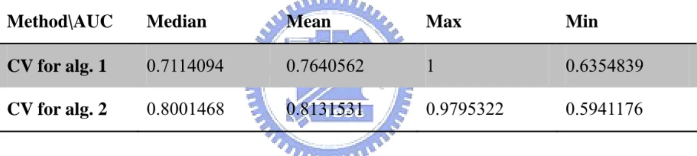
(22) From the CV results, most cases have hit rates that are at least 0.6 except a few of cases. Then, the overall average of all hit rates in algorithm 1 is 0.8912 and the overall average of all hit rates in algorithm 2 is 0.9279. We also try other strategies to further compare these two results of leave-one-out cross validation.. 4.2 Evaluating performances of two algorithms. There are 109 relationships in File-PD. So we have 109 results of cross validation in each cross validation. First, we compare two methods’ AUC (area under ROC curve, let y be power and x be type I error). There are 109 AUC in each method.. Table 1. Information about AUC of two algorithms under 109 cross validations Method\AUC. Median. Mean. Max. Min. CV for alg. 1. 0.7114094. 0.7640562. 1. 0.6354839. CV for alg. 2. 0.8001468. 0.8131531. 0.9795322. 0.5941176. 16.
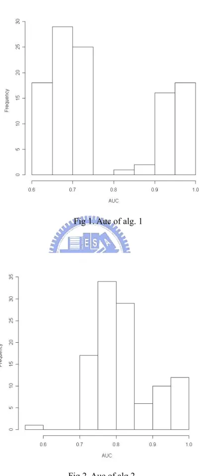
(23) Fig 1. Auc of alg. 1. Fig 2. Auc of alg.2. 17.
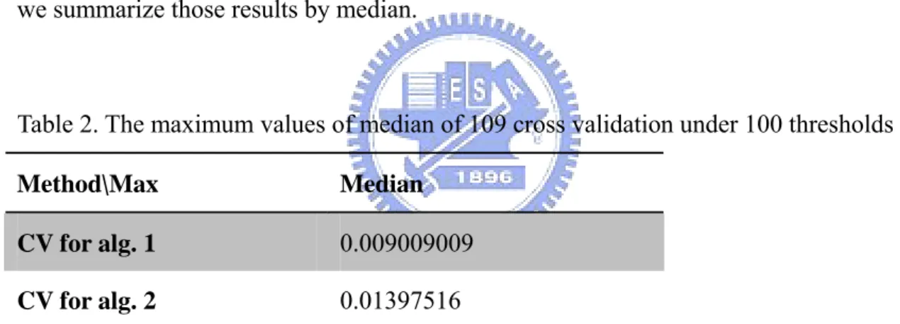
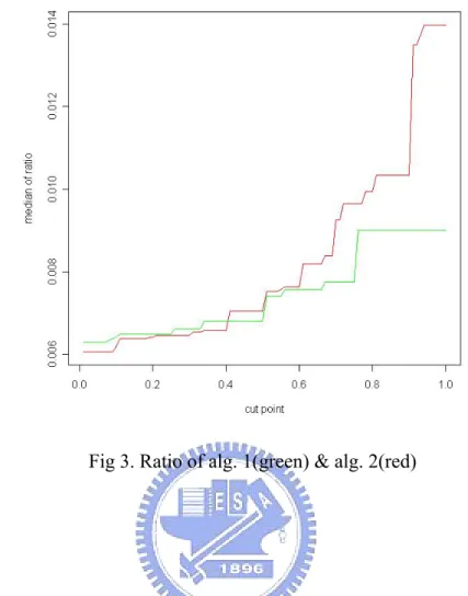
(24) From table 1, we can find that the performance of algorithm 2 is better than algorithm 1. But there is one questionable point that why we can decide type I and type II error without the knowledge about which gene truly associates with deficiencies. Furthermore, we are going to compare the ratio that we define as: covering ratio =. covering rate of known genes associated with a deficency the number of candidate genes. Each protein deficiency contains some gene deficiencies. The numerator of ratio indicates that gene deficiencies predicted by different thresholds divides the total number of gene deficiencies associated with this protein deficiency. By this definition, the larger ratio is, the better performance is. Because we hope the model can have a high covering rate and select less number of genes. Let cut points from 0.01 to 1. In each cut point, we have 109 ratios and we summarize those results by median.. Table 2. The maximum values of median of 109 cross validation under 100 thresholds Method\Max. Median. CV for alg. 1. 0.009009009. CV for alg. 2. 0.01397516. From table 2, the performance of algorithm 2 is still better than algorithm 1 in ratio. The conclusion of comparison algorithm 1 and 2 should be that algorithm 2 has a better performance than algorithm 1.. 18.
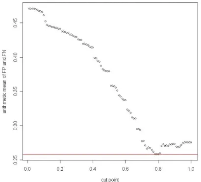
(25) Fig 3. Ratio of alg. 1(green) & alg. 2(red). 4.3 Threshold. In section 4.3, we talk about that we need to decide thresholds for those two algorithms. Here, we have three strategies to choose thresholds. First is controlling type I and type II error by arithmetic mean, second is finding the shortest distance by geometric mean and final is through observing the jump of the covering rate. First, let us control the type I and type II error by their arithmetic mean. There are 100 cut points from 0.01 to 1. Each point also contains 109 arithmetic means and we summarize information by taking average.. 19.
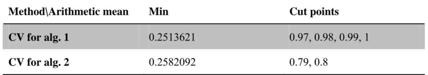
(26) Table 3. Thresholds and their corresponding arithmetic means in each algorithm Method\Arithmetic mean. Min. Cut points. CV for alg. 1. 0.2513621. 0.97, 0.98, 0.99, 1. CV for alg. 2. 0.2582092. 0.79, 0.8. Fig 4. Arithmetic mean of type I and type II error VS. cut point for alg. 1. 20.
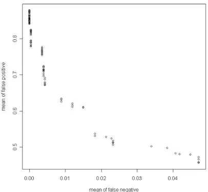
(27) Fig 5. Arithmetic mean of type I and type II error VS. cut point for alg. 2. Second, we find the shortest distance calculated by geometric mean of false positive and false negative.. Table 4. Thresholds and their corresponding geometric means in each algorithm Method\Distance. Min. Cut point. CV for alg. 1. 0.4580215. 0.97, 0.98, 0.99, 1. CV for alg. 2. 0.3869187. 0.89, 0.9. 21.
(28) Fig 6. Geometric mean of type I and type II errors VS. cut point for alg. 1. Fig 7. Geometric mean of type I and type II errors VS. cut point for alg. 2. 22.
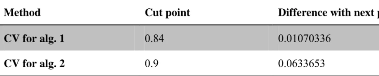
(29) Finally, we try to observe the change of covering rate, and find out the cut point which will make the covering rate change rapidly. This will mean that using the point might attain a lower number of candidate genes and an appropriate covering rate.. Table 5. Thresholds and their corresponding jumping ranges in each algorithm Method. Cut point. Difference with next point. CV for alg. 1. 0.84. 0.01070336. CV for alg. 2. 0.9. 0.0633653. Fig 8. Covering rate vs. cut point for alg. 1. 23.
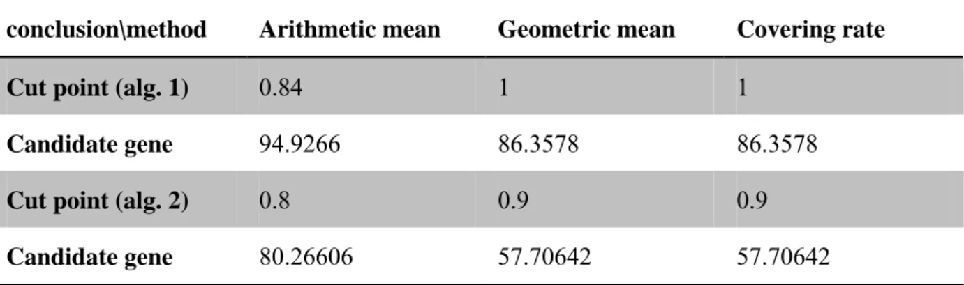
(30) Fig 9. Covering rate vs. cut point for alg. 2. Table 6. Information about thresholds and corresponding number of candidate genes in two alg. conclusion\method. Arithmetic mean. Geometric mean. Covering rate. Cut point (alg. 1). 0.84. 1. 1. Candidate gene. 94.9266. 86.3578. 86.3578. Cut point (alg. 2). 0.8. 0.9. 0.9. Candidate gene. 80.26606. 57.70642. 57.70642. 24.
(31) Chapter 5. Conclusion and Discussion. First, after deciding the threshold, we can construct a gene-disease deficiency qmr-like model. But it still lacks information to estimate model parameter. Maybe we can gather more data, but it is not easy because our data are depending on literature reports. New data need new PubMed publishes. So the next research orientation should be working on new method for tuning parameters of predicted models. Second, in our noisy-OR model, we ignore the “leak” and assume its inhibiting probabilities 1. But this assumption seems questionable, because this indicates that there are no any factors which will affect the diseases, excluding those genes we have known from literature reports. In order to complement this model, estimation of “leak” is a subject which we can keep working on. Although we have tried some statistic methods, the results are still so unconvincing. Furthermore, no matter which genes we choose, the most important thing is that we need a golden standard to compare with the results of our algorithms. If there are biological and experimental validations, then our results will be more persuasive.. 25.
(32) References. [1] Jensen FV. Bayesian Networks and Decision Graphs. Springer. 2001.. [2] Heckerman D. A tractable inference algorithm for diagnosing multiple diseases. Proceedings of UAI. 1989:174–181.. [3] Miller R, Masarie FE, Myers JD. Quick medical reference (QMR) for diagnostic assistance. MD Comput. 1986 Sep-Oct;3(5):34-48.. [4] Middleton B, Shwe MA, Heckerman DE, Henrion M, Horvitz EJ, Lehmann HP, Cooper GF. Probabilistic diagnosis using a reformulation of the INTERNIST-1/QMR knowledge base. II. Evaluation of diagnostic performance. Methods Inf Med. 1991 Oct;30(4):256-67.. [5] Neapolitan RE. Learning Bayesian Networks. Prentice Hall. 2004.. [6] Shwe MA, Middleton B, Heckerman DE, Henrion M, Horvitz EJ, Lehmann HP, Cooper GF. Probabilistic diagnosis using a reformulation of the INTERNIST-1/QMR knowledge base. I. The probabilistic model and inference algorithms. Methods Inf Med. 1991 Oct;30(4):241-55.. 26.
(33)
數據
+6
相關文件
甲型禽流感 H7N9 H7N9 H7N9 H7N9 H7N9 H7N9 H7N9 H7N9 - - 疾病的三角模式 疾病的三角模式 疾病的三角模式 疾病的三角模式 疾病的三角模式
存放檔案的 inode 資訊, inode 一旦滿了也一樣會 無法儲存新檔案, inode 會告知檔案所使用的 data block 位置。. Q :如何知道那些 inode 和
Unless prior permission in writing is given by the Commissioner of Police, you may not use the materials other than for your personal learning and in the course of your official
Place the code elements in order so that the resulting Java source file will compile correctly, resulting in a class called “com.sun.cert.AddressBook”。..
(D) It mounts all file systems listed in
In this project, we discovered a way to make a triangle similar to a target triangle that can be inscribed in any given triangle. Then we found that every triangle we’ve made in a
[r]
All the elements, including (i) movement of people and goods, are carefully studied and planned in advance to ensure that every visitor is delighted and satisfied with their visit,
