隨影像內容調整之移動估測加速技術

國 立 交 通 大 學

電 機 與 控 制 工 程 研 究 所

碩 士 論 文

隨影像內容調整之移動估測加速技術

A Content-Oriented Motion Estimation Speed-Up

Technique for Quasi-Stationary Video Compression

指導教授：董蘭榮 博士

研究生：陳泰佑

A Content-Oriented Motion Estimation Speed-Up

Technique for Quasi-Stationary Video Compression

Advisor: Dr. Lan-Rong Dung

Graduate Student: Tai-You Chen

July 2006

Graduate Institute of Electrical and Control

Engineering

National Chiao Tung University

Hsinchu, Taiwan, ROC

A Content-Oriented Motion Estimation Speed-Up Technique for

Quasi-Stationary Video Compression

Graduate Student: Tai-You Chen

Advisor: Dr. Lan-Rong Dung

Department of Electrical and Control Engineering

National Chiao Tung University

Abstract

In numbers of video compression standard, such as MPEG-1, MPEG-2, MPEG-4 and H.264/MPEG-4 AVC, motion estimation requires the most computational time and hence dominates main power requirement in video compression. Lots of published papers have presented efficient algorithms for simplifying motion estimation. But they don’t consider the influence of the video content. In our observation, the video content affects on the performance of motion estimation. So we base on the video content to select the suitable motion estimation in order to achieve a stable quality for most of video content. In this thesis, we develop an adaptive motion estimation algorithm with variable subsample ratios and this proposed algorithm can adaptively select the suitable subsample ratio for each current frame. The proposed algorithm also has been successfully implemented in the encoder model of H.264/MPEG-4 AVC reference software JM9.2. Experimental results has shown the proposed algorithm can not only adaptively select the suitable subsample ratio to various video sequences but also maintain ΔPSNRY of 0.5dB at most to save about 60.75% time for CIF sequences and 32.13% for D1 sequences of motion estimation in a fixed bit rate control on average.

隨影像內容調整之移動估測加速技術

學生：陳泰佑 指導教授：董蘭榮 博士

國立交通大學

電機與控制工程學系研究所

摘要

最新的影像壓縮規格中，如MPEG-1，MPEG-2，MPEG-4 and H.264/MPEG-4 AVC，移動估測需要龐大的移動估測時間與能量消耗。因此，移動估測主導了在 影像壓縮中的計算量與能量需求。針對移動估測，很多論文已經提出了不同的快 速演算法，可是他們並沒有考慮到影像內容的影響。在我們的觀察之下，影像內 容是會對移動估測的品質有所影響的。所以，我們根據影像內容來選擇適當的移 估測演算法，在大多數的影像內容都可以達到畫質穩定的效果。在此篇論文裡， 我們發展出一種利用變動取樣率可動態調整的移動估測演算法，並且此演算法可 針對每一張畫面內容的變動而動態選擇不同的取樣率。我們提出的這個演算法已 經成功的實現在H.264/MPEG-4 AVC的軟體模型JM9.2中，實驗結果顯示這個演算 法不只可以動態的依照不同的影像內容來選擇適合的取樣率，而且可以維持最多 0.5 dB的畫質衰退，在固定的傳輸頻率下，對於CIF解析度的影片平均可以節省 60.75％的移動估測時間,而對於D1解析度的影片則平均可以節省32.13％的移動 估測時間。

誌　 謝

首先，我要感謝董蘭榮老師在這兩年研究生涯中給予我的指導，

當我遇到困難時給予我適時的指點，讓我可以突破難關，順利完成此

論文。在生活上也受到董老師的關心與照顧，在此，獻上至高的謝意。

承蒙口試委員林進燈老師、陳宏銘老師、蔣迪豪老師，感謝您們

在百忙之中撥冗參與並給予我精闢的建議，謝謝你們寶貴的意見，使

我論文更加的完善。

感謝系統晶片實驗室的學長、同學以及學弟們，在我研究生涯裡

有你們的陪伴，是我努力向上的最大動力。感謝學長盟淳、松樹、芳

彥，同學岳璋、智偉、耕興、文豪，學弟信丞等，給我在課業與生活

上的幫助，有你們的陪伴，讓我有個充實的研究生活。

最後，我要深深的感謝養育我二十幾年的父母，讓我在求學過程

中無後顧之憂，並給予我鼓勵與支持，謝謝您們！

僅將本篇論文獻給所有愛我及我愛的人，再次獻上我由衷的感

謝，謝謝大家！

陳泰佑 謹誌

國立交通大學　系統晶片實驗室

民國九十五年七月

Contents

CHAPTER 1 INTRODUCTION ...1

CHAPTER 2 BACKGROUND ...6

2.1H.264/MPEG-4AVCVIDEO CODING SYSTEM...6

2.2BLOCK-BASED MOTION ESTIMATION...9

2.3SUBSAMPLE TECHNOLOGY... 11

2.3.1THE SUBSAMPLE ALGORITHM USING FIXED PATTERN...12

2.3.2THE SUBSAMPLE ALGORITHM USING ADAPTIVE PATTERN...16

2.3.3 GENERIC SUBSAMPLE ALGORITHM...21

2.4 HIGH-FREQUENCY ALIASING PROBLEM...24

2.5GOP-LEVELADAPTIVE MOTION ESTIMATION WITH VARIABLE SUBSAMPLE RATIOS... .26

CHAPTER 3 ADAPTIVE MOTION ESTIMATION WITH VARIABLE SUBSAMPLE RATIOS AT FRAME LEVEL...31

3.1PROPOSED ALGORITHM DEVELOPMENT...31 T 3.2 DEFINE TWO INDICES ZMBC IN TEMPORAL DOMAIN AND EC IN SPATIAL DOMAIN...34

3.3 ANALYZE VISUAL QUALITY DEGRADATION WITH SPATIOTEMPORAL CONDITION...36

3.4THRESHOLD DECISION FOR VARIABLE SUBSAMPLE RATIOS...44

CHAPTER 4 EXPERIMENTAL RESULT...52

CHAPTER 5 CONCLUSION...65

List of Figures

Fig 1.1: The proposed system diagram in H.264/MPEG-4 AVC encoder ...4 Fig 2.1: Rate-distortion curve comparison of H.264/MPEG-4 AVC with previous

standards (Excerpted from [21]) ...8 Fig 2.2: Subjective view comparison of MPEG-4 ASP (left) and H.264/MPEG-4 AVC

baseline (right) at bit-rate 112Kbps (Excerpted from [21])...9 Fig 2.3: Block diagram of H.264/MPEG-4 AVC encoder ...9 Fig 2.4: Block-based motion estimation ...10 Fig 2.5: Pixel patterns for decimation. (a) Full pattern with N×N pixels selected. (b)

Quarter pattern uses 4:1 subsample ratio. (c) Four-queen pattern is tiled with four identical patterns. (d) Eight-queen pattern. (c) and (d) are derived from the N-queen approach with N = 4 and N = 8, respectively (Excerpted from [14]) .13 Fig 2.6: (a) Patterns of pixels used for computing the matching criterion with a 4 to 1

subsample ratio. (b) Alternating schedule of the four pixel subsample patterns over the search area (Excerpted from [12]) ...14 Fig 2.7: Adaptive pixel selection (a) nine selected pixels. (b) The selected pixels in (a)

are considered as the central pixel for each region, the dotted lines indicate the neighbor pixels of respective central pixels in each region (Excerpted from [16])

...17 Fig 2.8: An edge in a 16×16 block for tested the subsample algorithm [17]...18 Fig 2.9: (a) 1-D Hilbert sequence converted from Fig.2.8. (b) Edge pixels detected

from 1-D Hilbert sequence. (c) 1-D row sequence converted from Fig.2.8. (d) Edge pixels detected from 1-D row sequence (Excerpted from [17]) ...20 Fig 2.10: The subsample patterns with 16:16, 16:8, 16:4 and 16:2 respectively...23

Fig 2.11: The results ΔPSNRY of the CIF tested video sequences ...23

Fig 2.12: The results ΔPSNRY of the D1 tested video sequences ...24

Fig 2.13: Frequency-domain illustration of down-sampling (Excerpted from [18])...25

Fig 2.14: The proposed system diagram for H.264/AVC encoder ...28

Fig 2.15: The diagram of ΔQ with 16:8, 16:4, 16:2 subsample ratios for the “Table” sequence (Excerpted from [26])...28

Fig 2.16: The ZMVC of the first P-frame in each GOP for the “Table” sequence (Excerpted from [26]) ...29

Fig 2.17: The statistical distribution of ΔGOPs versus ZMVC (Excerpted from [26]) ...30

Fig 3.1: The flowchart of the proposed algorithm ...34

Fig 3.2: (a) The ZMBC of “Table” (CIF) clip (b) The ZMBC of “Foreman” (CIF) clip………...…..….39

Fig 3.3: The ZMBC of “Football” (D1) clip………...….39

Fig 3.4: The RD curve of four subsample ratios at the 132th frame in “Table”...40

Fig 3.5: Logarithm scale curve fitting of the four RD curve ...40

Fig 3.6: The scene change occurrence (a)the 131st frame of “Table” sequence (b) the 132nd frame of “Table” sequence...41

Fig 3.7: The diagram of ΔQ with 16:8, 16:4 and 16:2 subsample ratios for “Table” sequence with rate control disable ...41

Fig 3.8: The ZMBC of the “Table” sequence...42

Fig 3.9: The EC of the “Table” sequence...42

Fig 3.10: The diagram of ΔQ with 16:8, 16:4 and 16:2 subsample ratios for “Foreman” sequence with rate control disable ...43

Fig 3.11: The ZMBC of the “Froeman” sequence...43

Fig 3.12: The EC of the “Foreman” sequence ...44

Fig 3.14: The five tested video sequences in D1 (720×480) resolution ...46

Fig 3.15: EC-ZMBC sample space of ten CIF clips ...47

Fig 3.16: Data and thresholds of subsample ratio 16:16...48

Fig 3.17: Data and thresholds of subsample ratio 16:8...48

Fig 3.18: Data and thresholds of subsample ratio 16:4...49

Fig 3.19: Data and thresholds of subsample ratio 16:2...49

Fig 3.20: The 80% threshold range for the four subsample ratios...50

Fig 4.1: The quality degradation of the proposed algorithm and generic subsample ratio for the CIF tested video sequence “Table” ...55

Fig 4.2: The quality degradation of the proposed algorithm and generic subsample ratio for the CIF tested video sequence “Foreman” ...55

Fig 4.3: The results ΔPSNRY of CIF tested video sequences and the proposed algorithm results location...63

Fig 4.4: The results ΔPSNRY of D1 tested video sequences and the proposed algorithm results location ...63

List of Tables

Table 2.1 Comparison of the sampling lattices an 8×8 block in measuring the directional coverage, four orientation described in Fig 2.5 (d) are used for horizontal, vertical and diagonal directions, there are eight, eight, and 15 possible edges, respectively, while for the diagonal directions, there are 15 possible edges (Excerpted from [14]) ...16 Table 2.2 Threshold setting for different condition under the 0.3 dB of visual quality

degradation (Excerpted from [26]) ...29 Table 3.1 Threshold Setting of the adaptive subsample ratio threshold decision for CIF

sequences ...50 Table 3.2 Threshold Setting of the adaptive subsample ratio threshold decision for D1

sequences ...51 Table 4.1 Tested video sequences and simulation conditions ...53 Table 4.2 Analysis of quality using adaptive subsample ratio decision for CIF tested

video sequences ...57 Table 4.3 Analysis of quality degradation using adaptive subsample ratio decision for

CIF tested video sequences...57 Table 4.4 The simulation results of average subsample ratio and overall average

subsample ratio for CIF tested sequences...58 Table 4.5 Analysis of quality using adaptive subsample ratio decision for D1 tested

video sequences ...58 Table 4.6 Analysis of quality degradation using adaptive subsample ratio decision for D1 tested video sequences ...59 Table 4.7 The simulation results of average subsample ratio and overall average

subsample ratio for D1 tested sequences ...59 Table 4.8 The PSNRY of the proposed algorithm and generic subsample ratio

algorithm for CIF tested video sequences...61 Table 4.9 The ΔPSNRY of the proposed algorithm and generic subsample ratio

algorithm for CIF tested video sequences...61 Table 4.10 The PSNRY of the proposed algorithm and generic subsample ratio

algorithm for D1 tested video sequences ...62 Table 4.11 The ΔPSNRY of the proposed algorithm and generic subsample ratio

Chapter 1 Introduction

In numbers of video compression standard, such as MPEG-1 [1], MPEG-2 [2], MPEG-4 [3] and H.264/MPEG-4 AVC [4], motion estimation requires the most computational time and hence dominates main power requirement in video compression. Lots of published papers [5] ~ [17] and [27] ~ [35] have presented efficient algorithms for simplifying motion estimation. But they don’t consider the influence of the video content. In other words, they can not keep the quality stable for different video sequence. In our observation, the video content affects on the performance of motion estimation. So we base on the video content to select the suitable motion estimation in order to achieve a stable quality for most of video content. We think that we must use the different motion estimation in the different video content. By the way, we can keep quality stable and save the motion estimation time simultaneously. Among many fast algorithms [5] ~ [17], the subsample algorithms [11] ~ [17] and [27] ~ [35] can not only easily combine with other approaches mentioned above but also reduce numbers of matching points with flexibly changing subsample ratio.

The subsample algorithm, also called the pixel decimation algorithm, in general, classified into two categories. One is fixed patterns [11] ~ [15], and the other is adaptive patterns [16] [17]. Bierling used an orthogonal sampling lattice with a 4:1 subsample [11]. Liu and Zaccarin implemented pixel decimation that is similar to Bierling’s approach with four alternating subsample patterns selected for each step so that all the pixels in the current block are visited [12]. T.Chiang et al presented an

N-queen decimation approach to address the spatial homogeneity and directional

luminance variation within a picture [16] [17]. The content-based subsample algorithm is proposed in [27] ~ [35]. Adaptive techniques can achieve better coding efficiency as compared to the uniform subsample schemes with an overhead in deciding which pattern is more representative. These presented subsample algorithms can successfully reduce the computational complexity of motion estimation to save much motion estimation time.

The reason why we choose the adaptive subsample ratios is because we believe that the subsample ratios should be varying with the video content. These subsample algorithms [11] ~ [15] are fixed patterns and they all don’t mention the spatial luminance variation within a picture. They result in serious aliasing problems in high frequency band to degrade the visual quality without considering the spatial variation. The spatial variation in the video means the degree of edge complexity. The degree of edge complexity is larger, and the spatial variation is stronger. Although the high subsample ratio cause aliasing in high frequency band, the degree of spatial variation will affect the degree of quality degradation. If the spatial variation is strong, aliasing problems will degrade the validity of motion estimation and result in visual quality degradation to video sequences obviously. On the contrary, if the spatial variation is weak, aliasing problems will not degrade the validity of motion estimation although the high subsample ratio still cause aliasing in high frequency band. That is because we do not need the high frequency band information to find the motion vector when the degree of object-moving is slow. Hence, using lower subsample ratio to reduce the prediction residual is necessary when spatial variation is stronger.

Although the subsample algorithms [16] [17] use the adaptive subsample patterns based on the spatial luminance variation within a picture, they don’t mention the temporal variation. They result in a serious problem to degrade the visual quality, because the motion estimation error would be propagated. If the temporal variation is

strong, the motion estimation results more residual. So, the encoder would let the quantization parameter larger to make the bit rate stable in fixed bit-rate control. In video compression, the big quantization parameter will result in visual quality degradation to video sequences obviously. On the contrary, if the temporal variation is weak, the visual quality degradation to video sequences is not obviously. Hence, using lower subsample ratio to reduce the prediction residual is necessary when temporal variation is stronger. In addition, scene change is a serious problem in the video compression. It will result a lot of residual when scene change occurs, and let quantization parameter rising immediately to bring out visual quality degradation obviously. The sudden degradation of visual quality will make the user uncomfortable, so we must detect the scene change phenomenon before encode one frame. We will propose a simple and effective method embedded in our algorithm.

In DSP theory [18] the subsample process will induce the aliasing in high frequency band. The aliasing problem affects the variance of the prediction residual under a fixed bit-rate constraint. The variance of the prediction residual affects the compression quality. The quality degradation of 0.5 dB is empirically reasonable for the perceptual tolerance of decompressed visual quality in video coding community. Therefore, in order to efficiently alleviate the aliasing problem to satisfy the visual quality under the quality threshold of 0.5 dB for general video sequences, adaptively selecting the suitable subsample ratio according to the degree of spatial and temporal variation in the content is imperative.

Current frame Reference frame Zero motion block counter Edge counter Subsample ME MC Choose intra prediction Intra prediction Filter T Q Q-1 T-1 Reorder Entropy encoder Inter Intra + + + -Coded bistream

Fig.1.1 The proposed system diagram in H.264/MPEG-4 AVC encoder

In this thesis, we develop an adaptive motion estimation algorithm with variable subsample ratios and this proposed algorithm can adaptively select the suitable subsample ratio for each current frame. Before this, there has been developed a group of picture (GOP) layer adaptive motion estimation algorithm with variable subsample ratios [26]. But it is not fine enough because it can not monitor video content change frame by frame immediately. The proposed algorithm is first to analyze the degree of the content in the spatial domain and temporal domain between the current frame and previous frame, then we can adaptively select the suitable subsample ratio to the current frame according to analysis results. The proposed algorithm also has been successfully implemented in the encoder model of H.264/MPEG-4 AVC [4] reference software JM9.2 [23] and the proposed system diagram is shown in Fig.1.1. The dash-lined region is the proposed motion estimation algorithm and the proposed algorithm offers four kinds of subsample ratios to switch adaptively. We use the statistics science to analyze the quality degradation of every frame, zero motion block counts (ZMBC) and edge counts (EC). And we get several different threshold values to experiment. The experimental results have been shown that the proposed algorithm

with the optimal threshold values can not only adaptively maintain visual quality under the quality degradation of 0.5 dB in a fixed bit-rate control for general video sequences but also meaningfully achieve the target of saving motion estimation time.

The rest of the thesis is organized as follows. We introduce the study background in chapter 2. In chapter 3, we describe the proposed algorithm. Chapter 4 shows the experimental performance of the proposed algorithm in H.264/MPEG-4 AVC [4] software model JM9.2 [23]. Finally, Chapter 5 concludes our contribution and merits of this work.

Chapter 2 Background

In this chapter, technical overview of H.264/MPEG-4 AVC [4] will be introduced [19] [20]. The feature of H.264/MPEG-4 AVC [4] different from MPEG-4 [3] will be pointed out [19] [20]. About the full-search algorithm, it is particularly attractive to ones who require extremely high quality. However, it requires a huge number of arithmetic operations and results in highly computational load and power dissipation. In order to reduce the computational complexity of the FSBM (full-search block-matching), lots of published papers [5] ~ [17] and [27] ~ [35] have presented efficient algorithms for motion estimation. Among these fast algorithms [5] ~ [17] and [27] ~ [35], the subsample algorithms [11] ~ [17] and [27] ~ [35] can not only easily combine with other approaches mentioned above but also reduce the number of matching points with flexibly changing subsample ratio. In general, the subsample algorithm, also called the pixel decimation algorithm, can be classified into two categories. One is fixed patterns [11] ~ [15], and the other is adaptive patterns [16] [17] and [27] ~ [35]. Adaptive techniques can achieve better coding efficiency as compared to the uniform subsample schemes with an overhead in deciding which pattern is more representative. These presented subsample algorithms [11] ~ [17] and [27] ~ [35] can successfully reduce the computational complexity of motion estimation to save much motion estimation time.

2.1 H.264/MPEG-4 AVC Video Coding System

H.264/MPEG-4 AVC [4] provides ultra high coding efficiency and network friendly functionalities. It has been a hot candidate for future video streaming and

communications. Fig.2.1 [21] shows that rate-distortion curve comparison of H.264/MPEG-4 AVC [4] with previous video coding standards. Under medium bit-rate, its PSNR quality outperforms MPEG-4 [3] simple profile by more than 3 dB. Fig.2.2 shows H.264 baseline subjective view comparison with MPEG-4 advanced simple profile at the specification of QCIF and bit-rate 112Kbps.

H.264/MPEG-4 AVC [4] has such high performance because it adopts several novel coding tools in its algorithm design. For example, variable block size motion estimation, multiple reference frame motion estimation, and intra frame prediction are used in its prediction algorithm. In-loop deblocking filter offers good subjective view. The 6-tap filter is incorporated to do the quarter pixel interpolation. CAVLC (Context-Adaptive Variable Length Coding) and CABAC (Context-Adaptive Binary Arithmetic Coding) are adopted in its entropy coding design. H.264/MPEG-4 AVC [4] is the first video coding standard that adopts the arithmetic coding into its entropy design. The block diagram of H.264/MPEG-4 AVC encoder is shown in Fig.2.3. Video frames are captured into intra prediction and inter prediction parts. If the frame type is intra, the inter prediction part will be disabled. Multiple reference frames and variable block size motion estimation is used for inter prediction. The best mode among these prediction modes is chosen in the mode selection block. The input frame is then subtracted from the prediction and forms the residue block. The residue blocks are transformed by 4×4 integer DCT for luminance and 2×2 transform for chrominance DC coefficient. Scan and quantization procedures are then applied to the coefficients. The entropy coder receives these quantized coefficients and generates codeword. The mode information is also transformed by the mode tables and fed into the entropy coder. The reconstruction loop includes the dequantization, inverse transform and deblocking filter. Finally, the reconstruct frame is written to the frame buffer for motion estimation.

There are three kinds of profile for H.264/MPEG-4 AVC standard [4]: baseline profile is for real-time communication, main profile is for digital storage application, and x-profile is for network streaming application. In the baseline profile, B-frame is not used and CAVLC is adopted in entropy coding. In the main profile, B-frame coding is used and CABAC is adopted for entropy coding. And X-profile has all the features of baseline profile while B-frame coding, SI-frame coding, and SP-frame [22] coding are included. Although the coding performance of H.264 is good, more than four times of the algorithm complexity compared to MPEG-4 simple profile prevents its practical implementation. Several previous papers and documents have addressed the coding complexity of this new state of art video coding algorithm.

Fig.2.1 Rate-distortion curve comparison of H.264/MPEG-4 AVC with previous standards (Excerpted from [21])

Fig.2.2 Subjective view comparison of MPEG-4 ASP (left) and H.264/MPEG-4 AVC baseline (right) at bit-rate 112Kbps (Excerpted from [21])

Fig.2.3 Block diagram of H.264/MPEG-4 AVC encoder

Next section, we will discuss the motion estimation, it is the most important part in the video encoder.

2.2 Block-based Motion Estimation

Motion estimation is the most important component in the video encoder and it directly affects the encoding speed and image quality. According to statistics, it consumes about 70% of the whole encoding time. Therefore, a good motion estimation algorithm can not only reduce the temporal redundancy of video sequence

but also get high quality of the reconstructed images. In the H.264/MPEG-4 AVC standard, motion estimation involves multiple prediction modes, multiple reference frames, and variable block sizes to achieve more accurate prediction and higher compression efficiency. However, the computational load of motion estimation increases greatly in H.264 because of the new features. In the H.264 codec, the motion estimation can consume 60%~80% of the total encoding time. Much higher proportion can be consumed if some optimization tools e.g. rate distortion optimization or a larger search range is used, but it can get higher quality.

Motion estimation of a macroblock involves finding a 16×16-sample region in a reference frame that closely matches the current macroblock. The reference frame is a previously-encoded frame from the sequence and may be before or after the current frame in display order. An area in the reference frame centered on the current macroblock position (the search area) is searched and the 16×16 region within the search area that minimizes a matching criterion is chosen as the ‘best match’.Fig.2.4

In a sequence of frames, the current frame is predicted from a previous frame known as reference frame. The current frame is divided into macroblocks, typically 16×16 pixels in size. This choice of size is a good trade-off between accuracy and computational cost. However, motion estimation techniques may choose different block sizes, and may vary the size of the blocks within a given frame.

Each macroblock is compared to a macroblock in the reference frame using some error measure e.g. MSE (mean square error), MAE (mean absolute error), or SAD (sum of absolute difference) and the best matching macroblock is selected. The search is conducted over a predetermined search area. A vector denoting the displacement of the macroblock in the reference frame with respect to the macroblock in the current frame is determined. This vector is known as ‘motion vector’.

When a previous frame is used as a reference, the prediction is referred to as forward prediction. If the reference frame is a future frame, then the prediction is referred to as backward prediction. Backward prediction is typically used with forward prediction, and this is referred to as bidirectional prediction.

In video compression schemes that rely on interframe coding, motion estimation is typically one of the most computationally intensive tasks. So, the subsample technique can alleviate the motion estimation computational load. We discuss it in the next section.

2.3 Subsample Technology

The subsample algorithm, also called the pixel decimation algorithm, it can not only easily combine with other approaches but also reduce numbers of matching points with flexibly changing subsample ratio. In general, it classified into two categories. One is fixed patterns [11] ~ [15], and the other is adaptive patterns [16]

[17]. For the fixed patterns, we can be sure that the time of the motion estimation will be down by subsample scale. But different patterns will case the different degree of quality degradations. For the adaptive patterns, can achieve better coding efficiency as compared to the uniform subsample schemes with an overhead in deciding which pattern is more representative. In the last, we present a generic subsample algorithm in which the subsample ratio ranges from 16:2 to 16:16. Because we believe that the subsample ratio should be varying with the video content. So we will apply that in the adaptive subsample ratio algorithm.

2.3.1 The Subsample Algorithm Using Fixed Pattern

Bierling used an orthogonal sampling lattice with a 4:1 subsample [11]. The pattern they used is the quarter pattern, shown in Fig.2.5 (b) [14]. The quarter pattern can save the motion estimation time for 75%. And the paper [12] uses four different quarter pattern to the different search area. They are based on motion-field and pixel subsample. They first determine a subsample motion field by estimating the motion vectors for a fraction of the blocks. The motion vectors for these blocks are determined by using only a fraction of the pixels at any searched location and by alternating the pixel subsample patterns with the searched locations. They then interpolate the subsample motion field so that a motion vector is determined for each block of pixels. Fig.2.6 (a) shows a block of 8×8 pixels with each pixel labeled a, b, c, or d in a regular pattern. We call pattern A the subsample pattern that consists of all the “a” pixels, as the quarter pattern. Similarly, patterns B, C, and D are the subsample patterns that consist of all the “b”, “c”, and “d” pixels, respectively. If only the pixels of pattern A are used for block matching, then the computation is reduced by a factor of 4. However, since 3/4 of the pixels do not enter to the matching

computation, the use of this subsample pattern alone can seriously affect the accuracy of the motion vectors. To reduce this drawback, they proposed using all four quarter patterns, but only one at each location of the search area and in a specific alternating manner. Fig.26. (b) shows some pixels forming part of the search region in the previous frame. The pixels are labeled 1, 2, 3, and 4 in a regular pattern. The labeling of the pixels refers to which of the four quarter patterns of Fig.2.6 (a) is to be used for computing the matching at that location. That is, when computing the match at locations labeled 1 (i.e., when the upper-left pixel of the block to match those locations), pattern A is used. Similarly, pattern B, C, or D is used when computing the match at locations labeled 2, 3, or 4.

Fig.2.5 Pixel patterns for decimation. (a) Full pattern with N×N pixels selected. (b) Quarter pattern uses 4:1 subsample ratio. (c) Four-queen pattern is tiled with four identical patterns. (d) Eight-queen pattern. (c) and (d) are derived from the

Fig.2.6 (a) Patterns of pixels used for computing the matching criterion with a 4 to 1 subsample ratio. (b) Alternating schedule of the four pixel subsample patterns

over the search area (Excerpted from [12])

We can analyze the subsample pattern with the spatial homogeneity and directional coverage [14]. The spatial homogeneity is measured by the average and variance of spatial distances from each skipped pixel to its nearest selected pixel where N is the dimension of the block, and indicates the coordinates of the selected pixel nearest to the pixel at the position . K is the number of the selected pixels. Smaller ) , ( yx S ) , ( yx d

μ and indicate a more spatially homogeneous sampling lattice. An edge is defined as a line passing through the sampling grids in any of , ,

and directions in Fig.2.5 (d). The directional coverage is measured as the percentage of edges that at least one of the selected pixels exists on an edge. Table 2.1 shows that the quarter pattern has less spatial homogeneity and lacks half of the coverage in the specified directions. To address the issues of spatial homogeneity and directional coverage, the paper [14] construct a new N-queen sampling lattice Fig.2.5 (c) and (d). 2 d σ ° 0 45° ° 90 135°

(

)

∑

∑

= = = = − − − = − − = N y x d d N y x d y x S y x K N y x S y x K N 1 , 1 2 2 2 1 , 1 2 ) , ( ) , ( ) ( 1 ) , ( ) , ( ) ( 1 μ σ μ (Excerpted from [14])

In the paper [14], to fully represent the spatial information of an N×N block, it is required that at least one pixel should be selected for each row, column, and diagonal. To satisfy such a constraint, the solution is identical to the problem of placing queens on a chessboard, which is referred to as N-queen pattern. For an N×N block, as shown in Fig 2.5 (c) and (d), every pixel of the N-queen pattern occupies a dominant position, which is located at the center. All the other pixels located on the four lines in the vertical, horizontal and diagonal directions are removed from the list of the selected pixels. With such elimination process, there is exactly one pixel selected for each row, column, and (not necessarily main) diagonal of the block. Thus, the N-queen patterns present a subsample lattice that can provide N times of speedup improvement. Despite the randomized lattice, the paper [15] designed compact data storage architecture for efficient memory access and simple hardware implementation for the N-queen patterns.

Table 2.1

Comparison of the sampling lattices an 8×8 block in measuring the directional coverage, four orientation described in Fig 2.5 (d) are used for horizontal, vertical and diagonal directions, there are eight, eight, and 15 possible edges, respectively, while for the diagonal directions, there are 15 possible edges (Excerpted from [14])

Spatial homogeneity Directional coverage (θ) Pattern d μ 2 d σ d d μ σ _{0 ° 45 ° 90 ° 135 °} Full 0 0 8/8 8/8 15/15 15/15 Quarter [11] 1.14 0.04 17.16% 4/8 4/8 7/15 7/15 Hexagonal [13] 1.03 0.11 11.07% 4/8 8/8 12/15 12/15 4-Queen [14] 1 0 8/8 8/8 10/15 10/15 8-Queen [14] 1.32 0.14 28.77% 8/8 8/8 8/15 8/15

2.3.2 The Subsample Algorithm Using Adaptive Pattern

The approach using the fixed patterns could possibly be able to obtain a good estimation of motion when the intensity of the block is nearly uniform. However, in the case of high activity blocks, some details may be neglected. Thus, it probably would introduce excessive prediction error. The paper [16] is based on the fact that high activity in spatial domain such as edges and texture mainly contributes to the MAD criterion. We can vary the number of selected pixels based on the image details. In other words, we can use fewer pixels when the block has uniform intensity. But in the high activity block, more pixels can be employed for the MAD matching criterion. This adaptive approach [16] can reduce the prediction error compared with standard pixel decimation [11] ~ [15]. In the algorithm [16], they used the relationship between

a pixel and its neighbors to select the most representative pixels. For example in 8×8 block size, initially, nine pixels are selected as shown in Fig.2.7 (a). The 8×8 pixel block is divided into nine regions, depicted in Fig.2.7 (b), and each region has its corresponding central pixel. In each region, the difference is defined the difference between central pixel and one of its neighbor pixels. If the difference is greater than threshold, this pixel is selected. We have used block size of 8×8 as an example for the description of the proposed algorithm in the paper [16]; however, the extension of the proposed scheme to a large block size, say 16×16, is straightforward.

k D k D K k k h k I h k I

D ( , )= ( , )− , where (h, k) is the location of the neighbor pixel in

region K, with (h, k) as the displacements from the central pixel . Ik

Fig.2.7 Adaptive pixel selection (a) Nine selected pixels. (b) The selected pixels in (a) are considered as the central pixel for each region, the dotted lines indicate the

neighbor pixels of respective central pixels in each region (Excerpted from [16])

Fig.2.8 An edge in a 16×16 block for tested the subsample algorithm [17]

About the paper [16], their scheme still requires an initial uniform division of a block, and therefore the pattern is locally adaptive. The pixel-decimation algorithm proposed in the paper [17] also utilizes edge information. Compared to Chan’s method [16], it extends the adaptively from local to global. To realize global adaptively, the algorithm [17] looks directly for edge pixels instead of requiring an initial uniform division of a block. This task [17] is made easier in a 1-D space with the help of Hilbert scan [37]. The Hilbert scan was named after the great German mathematician Hilbert, who found the simplest family of curves (Hilbert curves) that pass through all the grid points only once in a 2-D space [37]. The Hilbert scan, defined as a scan of a 2-D image through one of its Hilbert curves, is equivalent to a depth-first scanning of a quad-tree representation of the 2-D image. Some interesting features of this scan method used in previous applications include: 1) it is easier to extract clusters in an image with a Hilbert scan than other scan methods, e.g., row scan, row-prime scan, Morton scan, etc., and 2) it preserves 2-D coherence [38] ~ [43]. In addition, Kamata has shown that edge information in a 2-D image is preserved in its 1-D Hilbert-scan sequence, and has demonstrated an effective compression of 2-D images by compressing their 1-D sequences using the edge information [42]. The compressed images have a similar visual quality to that of the JPEG images at a high

compression rate.

To illustrate how edges are detected in a 1-D Hilbert sequence, Fig.2.8 shows a 2-D block with a closed circular edge, and Fig.2.9 (a) is the 1-D Hilbert sequence converted from the block in Fig.2.8. If edge pixels are defined at where pixel intensity changes the most, 22 edge pixels can be located in Fig.2.9 (a). All of the 22 pixels, when mapped back to 2-D, appear evenly distributed on the circular edge as shown in Fig.2.9 (b). For comparison, Fig.2.9 (c) is the 1-D row sequence converted from the same block in Fig.2.8. Although the row sequence contains 20 edge pixels, they all appear at the left and right vertical portion of the circular edge, and none appear on the upper and lower horizontal edges, as shown in Fig.2.9 (d). In general, the Hilbert scan not only provides edge information with little directional preference, but also preserves pixel coherence more effectively than other scan methods. In contrast, row scan, typical of many other scan methods, may miss edges due to its scan direction. Based on edge information in 1-D Hilbert sequences [37], the algorithm [16] selects pixels at which the matching criterion is evaluated.

Fig.2.9 (a) 1-D Hilbert sequence converted from Fig.2.8. (b) Edge pixels detected from 1-D Hilbert sequence. (c) 1-D row sequence converted from Fig.2.8. (d)

Edge pixels detected from 1-D row sequence (Excerpted from [17])

The paper [27] ~ [35] proposed that the general subsample algorithm has aliasing problem when it is in high subsample rate. The aliasing problem leads to considerable quality degradation because the high frequency band is messed up. To alleviate the problem, he uses edge extraction techniques to separate the edge pixels from a macro-block and then perform subsampling to the remaining pixels.

2.3.3 Generic Subsample Algorithm

We present a generic subsample algorithm in which the subsample ratio ranges from 16-to-2 to 16-to-16. The basic operation of the generic subsample algorithm is to find the best motion estimation with less SAD computation. The generic subsample algorithm uses Eq.2.1 as a matching criterion, called as subsample sum of absolute difference (SSAD), where the macroblock size is N-by-N, R(i,j) is the luminance value at (i,j) of the current macroblock (CMB). The S (i+u,v+j) is the luminance value at (i,j) of the reference macroblock (RMB) which offsets (u,v) from the CMB in the searching area 2p-by-2p. SM16:2m is the subsample mask for the subsample ratio

16-to-2m as shown in Eq.2.2 and the subsample mask SM16:2m is generated from basic

mask as shown in Eq.2.3. When the subsample ratios are fixed at powers of two because of regularly spatial distribution, these ratios are 16:16, 16:8, 16:4 and 16:2 respectively. These subsample masks can be generated in a 16-by-16 macroblock using Eq.2.3 and are shown in Fig.10. From Eq.2.3, given a subsample mask generated, the computational cost of SSAD can be lower than that of SAD calculation; hence, the generic subsample algorithm can achieve the target of saving the motion estimation time with flexibly changing subsample ratio. However, the generic subsample algorithm suffers aliasing problem for high frequency band. The aliasing problem will degrade the validity of motion vector (MV) and obviously result in visual quality degradation for some video sequences.

We use the fixed subsample ratio from 16:2 to 16:16 to experiment the eleven CIF and five D1 video sequences [37] in H.264/MPEG-4 AVC [4] coder with JM9.2 [23]. Here, we define one group of picture (GOP) is fifteen frames, the frame rate is 30 frames/s, the bit rate is 128k bits/s and initial Qp is 34. We can observe the quality degradation of the video sequences in the Fig.2.11 and Fig.2.12. In Fig.2.11 and

( )

( )

(

)

( )

Fig.2.12, the large quality degradation is caused at the higher subsample ratios and the lower subsample ratio cause small quality degradation. Hence, using lower subsample ratio to reduce the prediction residual is necessary when temporal variation or spatial variation is stronger. For those most stationary video sequences, we can use the highest subsample ratio to save the most motion estimation time. That is because the quality degradation is acceptable.

Therefore, we can conclude that we must use the different subsample ratio to keep the quality degradation acceptable. It is not enough to only use the fixed subsample pattern for all video sequences. Next section will describe how the high frequency aliasing problem occurs for subsample algorithm.

( )

16:2 1 1 16:2 0 0 16:2 , , , , , , 1 ( .2.1) , ( 1) ( 5) ( 2) ( 6) ( 7) ( 3) ( 8) ( 4) ( 2) ( 5) ( 1) ( 6) ( 7) ( 3) ( 8) ( 4) m SM N N m i j m SSAD u v SM i j S i u j v R i j p u v p Eq SM i j u m u m u m u m u m u m u m u m u m u m u m u m u m u m u m u m − − = = = ⋅⎡_⎣ + + − ⎤_⎦ − ≤ ≤ − = − − − − ⎡ ⎤ ⎢ _{− − − −} ⎥ ⎢ ⎥ ⎢ − − − − ⎥ ⎢ _{− − − −} ⎥ ⎣ ⎦

∑∑

( .2.2) 1, 0 ( ) ; , ( ) 0, 0 Eq for n where u n is a step function that is u n

for n ≥ ⎧ _{= ⎨} < ⎩

Fig.2.10 The subsample patterns with 16:16, 16:8, 16:4 and 16:2 respectively

Fig.2.12 The results ΔPSNRY of the D1 tested video sequences

2.4 High-frequency Aliasing Problem

The subsample process is like the down-sampling process in DSP theory [18]. In general, the operation of reducing the sampling ratio will be called down-sampling. Down-sampling is illustrated in Fig.2.13 We assume that the Fig.2.13 (a) is the conceptual spectrum of a macroblock in a frame of a video sequence. If this macroblock is down-sampling by 2, then his new conceptual spectrum will be Fig.2.13 (b). Because the original conceptual spectrum is low bandwidth and the down-sampling ratio is low, the aliasing don’t happen in this case. If the down-sampling ratio becomes 3, the aliasing will happen shown in Fig.2.13 (c). The aliasing in the high frequency band will case the motion estimation is no accurate. Aliasing problems affect the variance of the prediction residual under a fixed bit-rate constraint. The variance of the prediction residual affects the compression quality. Therefore, in order to efficiently alleviate aliasing problems to satisfy the visual

quality under the quality threshold of 0.5 dB for general video sequences, adaptively selecting the suitable subsample ratio according to the degree of spatial variation in the content is imperative.

According to sampling theory, the decrease of sampling frequency will result in aliasing problem for high frequency band. On the other hand, when the bandwidth of signal is narrow, lower downsample ratio or lower sampling frequency is allowed without aliasing problem. When applying the generic subsample algorithm for video compression, for high-variation frames, the aliasing problem occurs and leads to considerable quality degradation because the high frequency band is messed up.

The edge count (EC) is a good sign for the frame-level complexity detection because it is feasible for measurement. The large EC means that the spatial complexity is high. Hence, we can set low subsample ratio for large ECand high subsample ratio for small EC. Doing so, the aliasing problem can be alleviated and the quality can be frozen within an acceptable range.

(a) The original conceptual spectrum

(b) Down-sampling by 2

(c) Down-sampling by 3 (with aliasing problem)

2.5 GOP-Level Adaptive Motion Estimation with Variable Subsample

Ratios

The propose algorithm is aware of the motion-level of content and adaptively select the subsample ratio for each group of picture (GOP). Fig.2.14 shows the application of proposed algorithm. The dash-lined region is the proposed motion estimation algorithm and the proposed algorithm switches the subsample ratios according to the zero motion vector count (ZMVC). The larger ZMVC is used the higher subsample ratio. As the result of applying the algorithm for H.264/AVC applications, the proposed algorithm can produce stationary quality at the PSNR of 0.36 dB for a given bitrate while saving about 69.6% motion estimation time for FSBM, and save the PSNR of 0.27 dB and 62.2% motion estimation time for FBMA.

So, to efficiently maintain the visual quality for video sequences with variable motion levels, we propose an adaptive motion estimation algorithm with variable subsample ratios. The proposed algorithm determines the suitable subsample ratio for each GOP based on the ZMVC. The ZMVC is a feasible measure for indicating the motion-level of video. The larger ZMVC is the lower the motion-level. Fig.2.16 shows the ZMVC of the first P-frame in each GOP for the “Table” sequence. Comparing with Fig.2.15, we can see that when ZMVC is large the ΔQ is little for the subsample ratio of 16:2. For the third and seventh GOP, ΔQ becomes high and the ZMVC is relatively small. Thus, the ZMVC is a good reference index to determine the suitable subsample ratio.

In the procedure of the proposed algorithm, we determine the subsample ratio at the beginning of each GOP because the ZMVC of the first inter-frame prediction is the most accurate. Hence, we only calculate the ZMVC of the first P-frame for the subsample ratio and efficiently save the computational load of ZMVC. Note that the

ZMVC of the first P-frame is calculated by using 16:16 subsample ratio. Given the ZMVC of the first P-frame, the motion-level is determined by comparing the ZMVC with pre-estimated threshold values. The threshold values are decided statistically using popular video clips.

To set the threshold values for motion-level detection, we first built up the statistical distribution of ΔQ versus ZMVC for video sequences with subsample ratios of 16:2, 16:4, 16:8 and 16:16. Fig.2.17 illustrates the distribution. Then, we calculated the coverage of given PSNR degradation ΔQ. In this paper, the given ΔQ is 0.3 dB.

Rk,p% indicates the covered range of p% of GOPs having ΔQ less than 0.3 dB for

subsample ratio of 16:k. Accordingly, we set the threshold values for the use of subsample ratios. Table 2.2 finally shows the summary of threshold values for the quality degradation requirement of 0.3 dB.

About-mentioned, that is GOP level adaptive control. But it is not fine enough because it can not monitor video content change frame by frame immediately, and maintain it. If there is a very high motion in a GOP, the video content variance is very strong, and the GOP level technique doesn’t make sense at this time. Furthermore, scene change would not come up between two GOP; it could happen but not always. So, we change the GOP level to frame level adaptive control and consider spatial and temporal condition at the same time. We will propose our algorithm in the next chapter.

Current frame Reference frame Motion-level detection Scalable fast ME MC Choose intra prediction Intra prediction Filter T Q Q-1 T-1 Reorder Entropy encoder Inter Intra + + + -Coded bistream MV

Fig.2.14 The proposed system diagram for H.264/AVC encoder

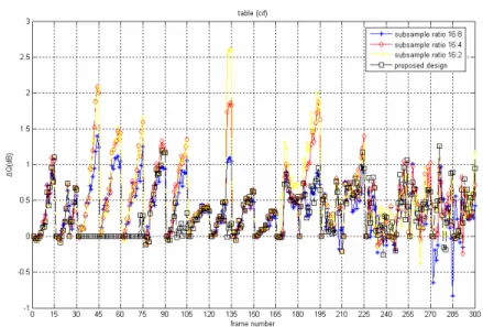
Fig.2.15 The diagram of ΔQ with 16:8, 16:4, 16:2 subsample ratios for the “Table” sequence (Excerpted from [26])

Fig.2.16 The ZMVC of the first P-frame in each GOP for the “Table” sequence (Excerpted from [26])

Table 2.2

Threshold setting for different condition under the 0.3 dB of visual quality degradation (Excerpted from [26])

The condition of percentage 90% 85% 80% 75% 70% 65% 60% Threshold of 16:2 (Th1) 393 387 376 344 305 232 190 Threshold of 16:4 (Th2) 368 356 344 251 239 190 49

Chapter 3 Adaptive Motion Estimation with

Variable Subsample Ratios in Frame Level

In this chapter, we describe the proposed algorithm in detail. We use one frame as a process unit, and get the zero motion block count (ZMBC) and edge count (EC) in the current frame. We must get the two motion indices before the current frame be encoded, because we want to predict how the temporal variation and spatial variation in the current frame earlier. According to these values of ZMBC and EC, we select the suitable subsample ratio for the current P-frame. Then the flowchart of the proposed algorithm is developed in Fig.3.1. Next, we provide four subsample ratios of 16:16, 16:8, 16:4 and 16:2 in order to let the proposed algorithm having better adaptive ability. The reason why to choose those subsample ratios is because they are symmetry and their scale is power of two. Final, we propose an adaptive subsample ratio threshold decision to set the compatible threshold values and get the optimal result. The static science is adopted in the adaptive subsample ratio threshold decision. We test the percentage of 95% to 60% in the statistically data of the quality degradation versus ZMBC and EC to get the different threshold value. From the result of eleven tested video sequences of CIF (352×288) resolution and five D1 (720×480) tested video sequences and we take the 85% result as the optimal threshold value.

3.1 Proposed Algorithm Development

To efficiently alleviate the aliasing problems in subsample algorithm to maintain the visual quality under the threshold of 0.5 dB for general video sequences, we propose an adaptive motion estimation algorithm using variable subsample ratios and

the proposed algorithm is based on the observation from Fig3.5 ~ Fig.3.10. The spatial variation in a frame is proportion to edge count (EC) and the temporal variation in a frame is in proportion to moving motion block count (MMBC), meaning that it is in inverse proportion to zero motion block count (ZMBC). Therefore, we use one frame as a processing unit and calculate the ZMBC and EC of P-frames in a tested video sequence. Next, we compare ZMBC and EC with threshold values to determine the suitable subsample ratio for the current frame. We recursively execute those steps above, and we can adaptively apply the suitable subsample ratio to each frame in the video sequence and also achieve the target of saving the motion estimation time.

A flowchart of the proposed algorithm is shown Fig.3.1 and the realization procedure of the adaptive motion estimation algorithm using variable subsample ratios is as follows.

Step 1: Setting initial value Set i=1.

We set the initial value in this proposed algorithm. And the proposed algorithm is ready to start

Step 2: Starting

When starting the proposed algorithm, the ith frame of the video sequence is picked out and goes to Step 3.

Step 3: Determining the current frame whether an I-frame or not

If the current frame is an I-frame, the proposed algorithm executes intra-frame coding to encode the current I-frame, and the current frame goes to Step 5; otherwise, the current frame is a P-frame and then goes to Step 4.

We can recognize the I-frame in the video sequence in this step. We don’t change the intra-predication in the proposed algorithm. Hence, the proposed algorithm

uses the same intra-prediction like H.264/MPEG-4 AVC for the I-frame.

Step 4: Adaptively selecting the suitable subsample ratio to the current P-frame The proposed algorithm compares ZMBC and EC of the P-frame with optimal threshold values to adaptively select a suitable subsample ratio and then uses this selected subsample ratio to execute inter-frame coding for the P-frame and then the current P-frame goes to Step 5. In order to guarantee the visual quality is good enough and can achieve the target accuracy. The priority of the compare order is to compare with 16:16 optimal threshold first, the second is to compare 16:8 optimal threshold, the third is to compare 16:4 optimal threshold and the rest use the 16:2 subsample ratio to encode it. The optimal thresholds are in the Table 3.1 and Table 3.2.

Step 5: Determining the current frame whether a last frame or not

If the current frame is the last frame, the procedure goes to Step 6; otherwise, the procedure sets i=i+1 and the next frame goes to Step 3.

Step 6: Ending

If all frames in the current video sequence are encoded, the proposed algorithm is finished. This video is end and all frames in the video sequence have been coded using the proposed algorithm in the H.264/MPEG-4 AVC [4].

start Selecting a frame

from the testing video sequence

Is this frame a I-frame

Intra prediction coding

Is this frame the last frame?

finish Next frame in the

testing video sequence Calculate the ZMBC and EC Does scene change occur?

Are ZMBC and EC in the circular Th16:16

Are ZMBC and EC in the circular Th_16:8

Are ZMBC and EC in the circular Th16:4 Inter prediction using 16:2 subsample ratio Inter prediction using 16:4 subsample ratio Inter prediction using 16:8 subsample ratio Inter prediction using 16:16 subsample ratio True True Fasle Fasle Fasle Fasle Fasle Fasle True True True True

Fig.3.1 The flowchart of the proposed algorithm

3.2 Define Two Indices ZMBC in Temporal Domain and EC in

Spatial Domain

We define the two indices which are ZMBC (zero motion block count) and EC (edge count). The ZMBC can reflect the video sequence spectrum in temporal domain and the EC can reflect that in spatial domain. In the encode system, we get the ZMBC and EC values before encoding, because we have to decide the subsample ratio before encoding. We use the higher subsample ratio for the larger ZMBC. Because of the

larger ZMBC means the frame has a small temporal variation with the reference frame. So, we choose the higher subsample ratio for it to be encoded, and we will not cause the error propagation problem but save the time of motion estimation simultaneously. On the other hand, we use the lower subsample ratio for the smaller ZMBC. The mechanism about how to choose the subsample ratio according to EC index is like the ZMBC index. We use the higher subsample ratio for the smaller EC. Because the smaller EC means the frame has a small spatial variation. So, we choose the higher subsample ratio for it to be encoded, and we will not cause the aliasing problem but save the time of motion estimation simultaneously. On the other hand, we use the lower subsample ratio for the larger EC to prevent the aliasing problem in the spatial domain.

The ZMBC is the difference between current frame and reference frame. In the beginning, we divide a frame into several blocks. And every block is size of 16×16 called macro-block (MB). Every current macro-block (CMB) is subtracted by the reference macro-block (RMB) which is at the same position in the reference frame to get ZMBC and we only calculate that at the position (0, 0). The basic operation to get the ZMBC is the sum of absolute difference (SAD). In our experience, we choose the threshold is 800 called ThZMBC. When a MB get the SAD is smaller than ThZMBC, it is

very likely to be a stationary MB so we define it is a zero motion block (ZMB). And we calculate how many ZMB in a frame, we can get the ZMBC. The lower bound of ZMBC in a frame is zero, but upper bound is the same number of MB in a frame. For example, in CIF (352×288) resolution the ZMBC upper bound is 396 and D1 (720×480) is 1350.

The other index in the spatial domain is EC which is sum of all edge pixels in a frame. Before calculating the EC, we must to extract the edge first. We want to detect where is edge and where is not, so we apply a popular gradient filter called as high

(

pass filter (HPF) Eq.3.1 to do the edge extraction. HPF can let the higher frequency band pass and filter out the lower frequency band. After the procedure of edge extraction, we can get gradient pixel values in a frame. And use the Eq.3.2 to calculate the ThEC. Then the algorithm uses the ThEC value as a condition to pick the edge pixels

produced by Eq.3.3. Finally we sum all the edge pixels in a frame to get the EC value.

)

( )

(

)

1 1

(

) (

)

1 1 ( , ) , ( , ) 1 1 1 1 8 1 1 1 1 , , 1, 1 1, 1 3 ( , ) ( , ) p q G i j MF HPF R i j where HPF MF M R i j M p q R p q where M is a by mask

R i j is the luminance value at i j

=− =− = − − − ⎡ ⎤ ⎢ ⎥ = −_⎢ − _⎥ ⎢− − − ⎥ ⎣ ⎦ = + + ⋅ + + 3− −

∑ ∑

(Eq.3.1)

( )

{

}

{

( )

}

1 2 1 2 max , min , 0.2, 0.8 EC Th m G i j m G i j where m m = ⋅ + ⋅ = = (Eq.3.2) 1, ( , ) ( , ) 0, EC for G i j Th E i j otherwise ≥ ⎧ = ⎨ ⎩ (Eq.3.3)

After we get the two indices ZNBC and EC, we will analyze the relation between quality degradation and the two indices at next section.

3.3 Analyze Visual Quality Degradation with Spatiotemporal

Condition

function named rate control. If we turn on this function, we can set a fixed target bit-rate and the encoder system will vary the Qp to fit the target bit-rate. It is a good approach for many portable devices and storage mechanisms. But the varied Qp would cause the frame quality vary together. In another word, the frame quality can not express itself content behavior accurate under the rate control enable. In order to solve this problem, we disable the rate control function, and scan the Qp from 2 to 42. At each Qp, we can get its own quality degradation and encoded bit-rate in a frame. Then we can use these two data to draw the RD curve (rate-distortion curve) in Fig.3.2, every frame has its own RD curve. We must to do curve fitting to get the quality at a constant bit-rate for these four subsample ratios. But, from the observation of these sample data, they are not distributed linearly, it like a logarithm scale distribution. So, we use logarithm scale to do the curve fitting with that like Fig3.3. In our simulation, we keep a constant bit-rate 128k bits/sec, and then we calculate the quality degradation difference between full search and other subsample ratios using the Eq.3.4. However, we get the quality degradation curve in a video sequence like Fig.3.5 and Fig.3.8.

ith frame i FSME SSR

Q =PSNRY −PSNRY

+ (Eq.3.4)

We take the video sequences “Table” and “Foreman” for examples. To particularly analyze the results of visual quality degradation with different subsample ratios for a video, the video sequences “Table” and “Foreman” are simulated in H.264/MPEG-4 AVC [4] coder with JM9.2 [23]. Here, we defined one group of picture (GOP) is fifteen frames, video sequence type is IPPP…, frame rate is 30 frames/sec and the bit rate is 128k bits/sec. Subsample ratios are 16:8, 16:4 and 16:2

respectively and can be generated from Eq.2.3, We analyze the “Table” video sequence first. Fig.3.5 shows quality degradation results versus these subsample ratios. Fig.3.6 shows the ZMBC value of every frame in the “Table” video sequence, and Fig.3.7 shows the EC value. From Fig.3.6 , there exists the strong temporal variance between the 20th frame to the 105th frame, hence, the higher subsample ratios result in more obviously higher quality degradation. Furthermore, the 132nd frame has the maximum quality degradation because of scene change (Fig.3.4). To deal with that problem, we also can use the temporal index; the ZMBC is extremely small at this time. Base on our observation, in most CIF clips when scene change occur, the ZMBC is smaller than 10. Fig.3.2 (a) and (b) are the ZMBC of “Table” clip and the ZMBC of “Foreman” clip. We define it, when ZMBC is smaller than 10, the scene change must happen. In D1 clips, “Football” sequence is a very fast motion clip and its motion is not regular (Fig.3.3). The “Football” motion is sometimes fast and sometimes slow, so the ZMBC value in “Football” is changed seriously. So we consider the phenomenon is also a kind of scene change. The D1 (720×480) resolution is larger than CIF (352×288), it has 1350 MBs. So we choose the scene change threshold as 100 for all D1 clips. According that, we apply low subsample ratio for this frame to be encoded. From Fig.3.7, there we can detect the spatial variance increasing gradually the 60th frame and the 105th frame, and the higher subsample ratios also degrade higher and higher. About the “Foreman” tested sequence from Fig.3.8 , there exists the strong temporal variance between the 170th frame to the 195th frame and the 225th frame to the 255th frame in the Fig.3.9, hence, the higher subsample ratios result in more obviously higher quality degradation. From Fig.3.10, there exists the strong spatial variance between the 240th to the 300th frame. Hence, the higher subsample ratios result in higher quality degradation. So, we will choose the low subsample ratio to encode these frames.

Above-mentioned, we simulate for observation in the relation between the quality degradation and spatiotemporal condition. In order to simulate the adaptive algorithm, we must have some thresholds for according to. In the next section, a threshold decision for variable subsample ratios will be presented.

(a) (b)

Fig.3.2 (a) The ZMBC of “Table” (CIF) clip (b) The ZMBC of “Foreman” (CIF) clip

Fig.3.4 The RD curve of four subsample ratios at the 132th frame in “Table” sequence

(a) (b)

Fig.3.6 The scene change occurrence (a) the 131st frame of “Table” sequence (b) the 132nd frame of “Table” sequence

Fig.3.7 The diagram of ΔQ with 16:8, 16:4 and 16:2 subsample ratios for “Table” sequence with rate control disable

Fig.3.8 The ZMBC of the “Table” sequence

Fig.3.10 The diagram of ΔQ with 16:8, 16:4 and 16:2 subsample ratios for “Foreman” sequence with rate control disable

Fig.3.12 The EC of the “Foreman” sequence

3.4 Threshold Decision for Variable Subsample Ratios

To support a suitable subsample ratio to each P-frame of a video sequence, an adaptive subsample ratio threshold decision is necessary. Therefore, we use 16:2, 16:4 and 16:8 subsample ratios respectively to statistical distribution of ZMBC versus EC for the ten CIF video sequences. We do the statistical distribution don’t include the “Stefan” sequences data because its EC values are too large. If we include “Stefan” data, it would cause large variation to influence our analysis. We first set the quality degradation threshold is 0.3 dB. We choose the nearest and not exceed the threshold subsample ratio for the frame. Furthermore, we want to achieve the target of saving the motion estimation time. We not only satisfy above two criterions but also choose the highest subsample ratio for the frame. By the way, if all subsample ratios are all exceeding the threshold, we choose the 16:16 subsample ratio for the frame. D1 also use the same way. For example, in Fig.3.8 the 40th frame is applied to 16:4 subsample

ratio and the 190th frame is applied to 16:16.

We take eleven CIF clips (Fig.3.11) and five D1 clips (Fig.3.12) to do the simulation for observation in the relation between the quality degradation and spatiotemporal condition. We can plot the EC-ZMBC sample space like Fig.3.13. Fig.3.14 to Fig.3.17 are the different four subsample ratio sample space with their eight circular thresholds. The center point of the circular threshold is the average value of all the data in the space (Eq.3.5) and the radius is positive proportion to the precision of the threshold decision. In the software, we first calculate all the distances between sample data and center point and sort all the distances up to down. According to thresholds and find the last point in the region. The distance of the last point from the center pint is the radius of the threshold. The X-axis radius is the EC value of the last point, and the Y-axis radius is the ZMBC of the last point. The circular threshold would include the percentage numbers of data according to the statistics. Table 3.1 shows the threshold centers and radiuses in every subsample ratio for CIF sequences and Table 3.2 shows the threshold centers and radiuses in every subsample ratio for D1 sequences. Furthermore, it is well to use circle shape as the threshold, because every point on the threshold edge keep the same distance from the center and it is friendly to the software coding.

In order to guarantee the visual quality is good enough and can achieve the target accuracy. The priority of the compare order is to compare with 16:16 optimal threshold first, the second is to compare 16:8 optimal threshold, the third is to compare 16:4 optimal threshold and the rest use the 16:2 subsample ratio to encode it. Furthermore, we draw the ranges covered by these four subsample ratios. In Fig.3.18, we can observe an interesting phenomenon that is the relation of subsample ratios and ZMBC is most closely than the relation of subsample ratios and EC. So, the circular thresholds would bend to ZMBC when subsample ratio lower and lower.

“Akiyo” “Children” “Dancer” “Foreman” “News”

“Silent” “Table” “Tempete” “Waterfall” “Weather”

“Stefan”

Fig.3.13 The eleven tested video sequences in CIF (352×288) resolution

“Character” “Coastguard” “Football”

“Mobile” “Night”

Fig.3.15 EC-ZMBC sample space of ten CIF clips 16:2 16:2 16:2 16:2 , 16:2m m m subsample ratio

subsample ratio subsample ratio

m m

center point

all sample points EC value all sample points ZMBC value all subsample ratio sample points all subsample ratio sample

=

∑

∑

1, 2, 4,8 points m ⎛ ⎞ ⎜ ⎟ ⎜ ⎟ ⎜ ⎟ ⎝ ⎠ = (Eq.3.5)

Fig.3.16 Data and thresholds of subsample ratio 16:16

Fig.3.18 Data and thresholds of subsample ratio 16:4

Fig.3.20 The 80% threshold range for the four subsample ratios

Table 3.1

Threshold Setting of the adaptive subsample ratio threshold decision for CIF sequences

The adaptive subsample ratio threshold decision of CIF sequences

95% 90% 85% 80% 75% 70% 65% 60% Center point (3070.40,99.59) X-axis radius 4551.75 4549.88 4479.75 4432.88 4233.75 2315.59 2064.53 2002.50 Threshold of 16:16 Y-axis radius 121.38 121.33 119.46 118.21 112.90 61.75 55.05 53.40 Center point (5719.50,187.00) X-axis radius 4854.38 4427.63 4182.38 3958.50 3813.75 3536.70 3289.65 2905.61 Threshold of 16:8 Y-axis radius 129.45 118.07 111.53 105.56 101.70 94.31 87.72 77.48 Center point (5205.40,220.31) X-axis radius 8161.13 4311.38 3843.38 3639.79 3500.36 3387.49 3223.43 3077.55 Threshold of 16:4 Y-axis radius 217.63 114.97 102.49 97.06 93.34 90.33 85.96 82.07

Table 3.2

Threshold Setting of the adaptive subsample ratio threshold decision for D1 sequences

The adaptive subsample ratio threshold decision of D1 sequences

95% 90% 85% 80% 75% 70% 65% 60% Center point (11712 , 285.51) X-axis radius 10980.64 9984.48 9039.80 8086.76 7234.48 6525.20 5930.76 5195.96 Threshold of 16:16 Y-axis radius 249.56 226.92 205.45 183.79 164.42 148.30 134.79 118.09 Center point (31517 , 133.40) X-axis radius 21474.64 20619.28 19343.28 18857.08 18153.52 17105.00 16713.84 16162.96 Threshold of 16:8 Y-axis radius 488.06 468.62 439.62 428.57 412.58 388.75 379.86 367.34 Center point (35275 , 100.80) X-axis radius 27423.88 23480.16 16224.12 13332.00 11940.28 11187.00 9889.44 9202.16 Threshold of 16:4 Y-axis radius 623.27 533.64 368.73 303.00 271.37 254.25 224.76 209.14