運用AdaBoost車輛檢測之特性和校正的事件分類

國

立

交

通

大

學

電控工程研究所

碩

士

論

文

Road Objects Classification with Camera Calibration

and Adaboost-based Vehicle Detector

AdaBoost

Road Objects Classification with Camera Calibration

and Adaboost-based Vehicle Detector

Student

Ting-Yi Chang

Advisor

Chin-Teng Lin

A Thesis

Submitted to Department of Electrical and Control Engineering College of Electrical Engineering

National Chiao Tung University in Partial Fulfillment of the Requirements

for the Degree of Master in

Electrical and Control Engineering July 2011

Road Objects Classification with Camera Calibration and

Adaboost-based Vehicle Detector

Student

Ting-Yi Chang

Advisors

Prof. Chin-Teng Lin

Institute of Electrical and Control Engineering

National Chiao Tung University

ABSTRACT

Visual-based vehicle detection techniques applied to Intelligent Transportation System (ITS) to improve the efficiency and precision of analyzing heavy video information have been studied for years. In this study, we take advantage of AdaBoost algorithm’s accurate detection rate cooperate with Gaussian Mixture Model (GMM) and calibration method we proposed to do classification. We transform the raw color image into a gray level image and resize it for acceleration. After resizing, the image is send to Gaussian mixture model (GMM) approach to obtain reliable background images, and then use background subtraction technique to extract foreground objects. In this stage, we use calibration for transferring pixel coordinates to world coordinates and cooperate with foreground subtracted by GMM to get and record foreground’s information, such as width and height for further classification. Here, we use concept of overlapping area for tracking and recording foreground’s information. For classification’s criteria, the AdaBoost vehicle detector uses slicing window to detect vehicles and verifies whether the foreground subtracted by GMM [22] [23] is vehicle. Through AdaBoost vehicle detector, we can separate vehicles from

pedestrians, motorcycles, and objects. Next, we utilize width and height ratio, edge complexity, and speed get from calibration to separate pedestrians and motorcycles from objects. Because we found that pedestrians and objects have different edge complexity range.

The objective of this study is to classify vehicles, pedestrians, and objects which include AdaBoost vehicle detector and calibrating the foreground’s width, height, and speed. Therefore, the system can warns us of the dangerous situation to protect both drivers and pedestrians. The experimental results proved the proposed system achieved a good performance of classifying vehicles, pedestrians, and objects. The implemented system also extracted useful traffic information that can be used for further processing, like classifying vehicles, ex: sedan, truck, bus, and classifying pedestrians and motorcycles by adding auxiliary features.

Table of Contents

... I ABSTRACT ... II ... IV Table of Contents ... V List of Figures ... VII List of Tables ... VIII

Chapter 1 Introduction ... 1

1.1 Motivation ... 1

1.2 Objective ... 3

1.3 Organization ... 3

Chapter 2 Related Works ... 4

2.1 Calibration Methods ... 4

2.2 AdaBoost Algorithm’s Application ... 6

Chapter 3 Road Objects Classification System ... 7

3.1 System Overview ... 7

3.2 Vehicle Detection using AdaBoost ... 8

3.2.1 Haar Features (Rectangle Features) ... 9

3.2.2 Weak Classifier ... 11

3.2.3 AdaBoost Algorithm ... 12

3.2.4 Cascaded Classifier... 16

3.2.5 Scan Window Size ... 19

3.3 Calibration Algorithm ... 21

3.3.1 Concept of Calibration ... 21

3.4 Classification ... 24

3.4.1 Method of Recording Foreground’s Information ... 24

3.4.2 Edge Complexity ... 26

3.4.3 Classification Criteria ... 27

Chapter 4 Experimental Results ... 29

4.1 AdaBoost Training ... 29

4.2 Results of Detecting Vehicles in Video ... 33

4.3 Results of Classification in Video ... 36

Chapter 5 Conclusions and Future Work ... 39

List of Figures

Figure 3-1 System diagram ... 8

Figure 3-2 The Haar-like features [5] ... 10

Figure 3-3 Integral image ... 10

Figure 3-4 Selecting thresholds for weak classifiers ... 11

Figure 3-5 The process of selecting and combining weak classifiers ... 15

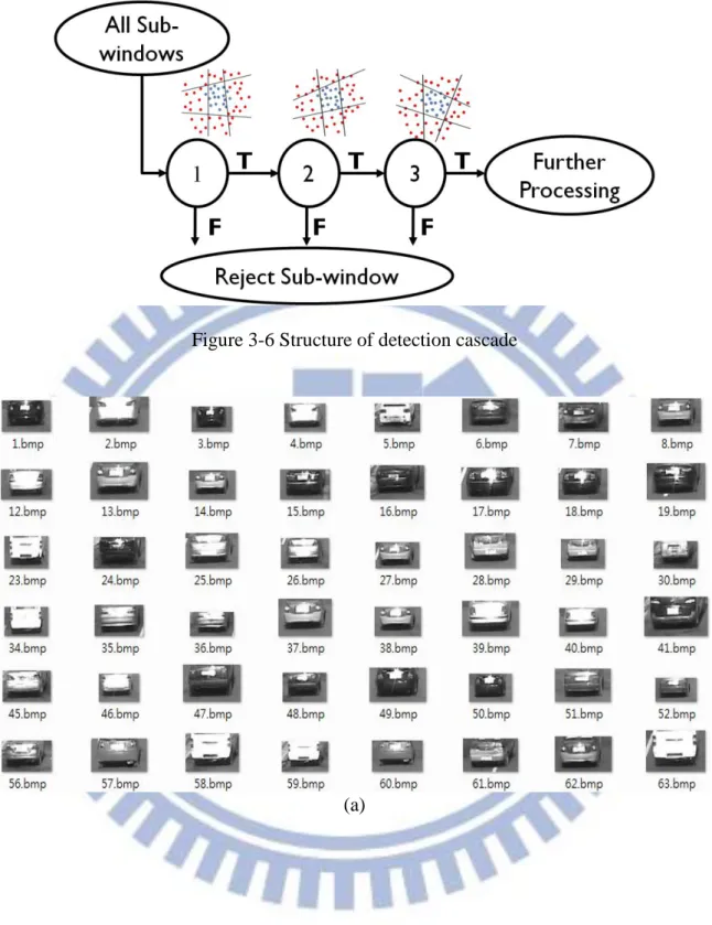
Figure 3-6 Structure of detection cascade ... 17

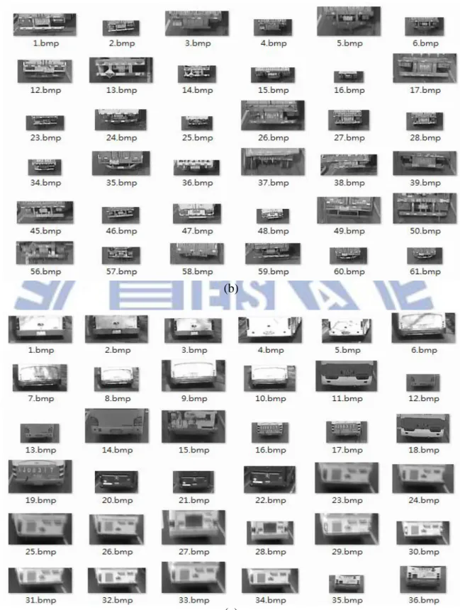
Figure 3-7 Some positive training samples of (a) Sedan and SUV (b) Truck (c) Bus ... 18

Figure 3-8 Some negative training samples ... 19

Figure 3-9 As vehicles continuously move, the size of vehicle is perspectively shrinked. ... 20

Figure 3-10 Width of vehicle at different position ... 20

Figure 3-11 Trajectory. ... 25

Figure 3-12 Diagram of recording foreground’s information ... 25

Figure 3-13 Some examples of edge image ... 27

Figure 3-14 Classification stages ... 28

Figure 4-1 Diagram of extracting vehicle samples ... 30

Figure 4-2 Some collected positive and negative samples ... 32

Figure 4-3 Flow chart of AdaBoost training process ... 32

Figure 4-4 Captured pictures of detection result ... 35

List of Tables

Table 3-1 The boosting algorithm for selecting and combining weak classifiers [11] ... 15

Table 3-2 The training algorithm for building a cascaded detector[11]. ... 16

Table 4-1 Detection rate, false alarm, and FPS between different scenes ... 33

Table 4-2 Detection rate, false alarm, and FPS between different scenes ... 33

Chapter 1 Introduction

1.1

Motivation

In recent years, video and image processing techniques have attracted great attention in computer vision for their applications to improve safety and convenience of human’s life. For instance, how to monitor and control the traffic condition efficiently with advanced techniques is one of the most important issues among the developed countries. Traditional traffic surveillance systems use sensors, namely analog equipment to detect vehicles and assemble simple information. The drawback is we have to check and analyze the information manually. This method is inefficient in information extraction, short of improving, and time consuming. On the other hand, digital cameras are cheaper and techniques of computer vision have been improved. Hence, visual-based Intelligent Transportation System (ITS) has attracted great attention recently. For example, video-based automatic surveillance system, vehicle behavior analysis system, accident prediction system, traffic monitoring system etc. are presented in many applications and products.

According to the National Highway Traffic Safety Administration, an average of nearly 5,000 non-motorists is killed on U.S. roadways each year. Twelve percent of casualties in traffic accidents are pedestrians in the United States. In European, more than 6000 pedestrians are killed and more than 150,000 are injured yearly. In 2004, 99,217 persons were killed in traffic accidents in China, and one third of them were pedestrians. Therefore, accurate and real-time pedestrian detection is important for us to avoid and reduce fatal accidents. That is to say, pedestrian protection is an important issue for us because of the high incidence of pedestrian accidents. In this paper, we propose a vision-based system that can recognize

situation to protect both drivers and pedestrians. Different sensor technologies, such as ultrasonic sensor, laser scanner, and cameras, are utilized to detect pedestrians [21]. Each technique has its own advantages and disadvantages. Among them, detecting pedestrians or other things by video camera is the most neat and tidy way because it brings no pollution to our environment and dose no harm to us. Besides, it’s the most similar way to human visual perception system. Vision-based detection gives a dependable method to guarantee us driving safety and prevent the traffic accidents. However, it’s still an open challenge due to many difficulties, such as complex and changeable environment, various pedestrian pose. Because complex computations are required in image processing, how to get quick result in detection remains a tough task. Since usually we are more interested in moving objects, we can perform background subtraction first and detect objects of interest only in the foreground regions. In this way the computation is reduced significantly.

1.2

Objective

The objective of this study is to construct a vehicle, pedestrians, and objects classification system. We cooperate AdaBoost vehicle classifier with calibration method we proposed to do road objects classification.

We propose to develop a road objects classification system that has these characteristics: 1. Can detect various kinds of back-viewed vehicles in a scene.

2. Can classify pedestrians, vehicles, and objects.

1.3

Organization

This thesis is organized as follows: Chapter II gives an overview of related works about this research. Chapter III presents the main modules of proposed system and explains details algorithm used in each module. Chapter IV shows experimental results and performance comparison. Finally, the conclusions of this study are stated in Chapter V.

Chapter 2 Related Works

2.1

Calibration Methods

The Camera calibration is a major work in computer vision, robotics, computer-integrated manufacturing systems, and automation. Camera calibration is the estimation and determination of some parameters necessary to establish projection equations between world coordinates and pixel coordinates. Camera self-calibration techniques make it possible to compute three-dimensional world coordinates of observed scene from video sequences without getting knowledge of the camera intrinsic parameters previously. The notion of self-calibration was introduced by Maybank and Faugeras for the perspective camera and by Hartley for the rotating camera. A self-calibration method for affine camera was given by Long. Over the past few decades, considerable endeavor has been made on development of effective and accurate procedures and algorithms to transfer the pixel coordinates to world coordinates, that is to say, identify the internal camera geometric and optical characteristics (intrinsic parameters) or the three-dimensional position and orientation of the camera frame relative to a certain world coordinate system (extrinsic parameters). In our study, camera calibration is based on the vanishing point of two lines known to be parallel on the road surface. Most work in camera calibration involves calibrating both intrinsic and extrinsic camera parameters simultaneously. However, real-time information is critical in many situations for successful applications. Accordingly, an efficient extrinsic parameters calibration algorithm that requires less preparation in manually operation setup and less computation in processing would be extremely useful.

Most calibration methods [12]-[15] use known features in a scene to evaluate the camera parameters, in [12], the calibration procedure is based on using the Camera Calibration

Toolbox for Matlab [24]. A calibration equation that separates rotational and translational parameters is given in [13]. In [13], a four-point calibration procedure is proposed that includes three points on a line and one point out of the line, and results in four possible calibration solutions, obtained analytically. For the reason of simplicity, in [13], it has been assumed that the camera world coordinates and the image coordinate axes are identical, and Z and z are the optical axis of the camera. In [14], it has presented a camera self-calibration technique which is able to handle time-varying focal length change. It has been exhibited that this technique can track focal length change even under relatively noisy conditions; however, it still uses known features in a scene to evaluate the camera parameters. In [16] and [17], sets of parallel lines of a hexagon are employed to calculate the camera parameters. Results from these papers show that parallel lines can be used to appropriately determine the camera parameters. Efficient algorithms [18]-[20] have been developed for evaluating the camera parameters utilizing parallel lanes in a traffic scene. In [18], a calibration algorithm for a single camera overlooking traffic is proposed. That algorithm needs the technician installing that system, measuring the height and tilt of the camera, and selecting the road edges in an image. That is to say, their method needs particular manual operations to measure the tilt angle of the camera. It shows how the camera calibration parameters can be computed from the height, the tilt, and the four selected points. Multiple parallel lanes and a particular perpendicular line were used to calibrate the camera parameters in [19] and [20]. Another method is to use special calibration targets to substitute for measurement of corresponding points. In this case; however, the calibration target must still be carefully installed relative to the world frame.

In this paper, a novel equation will be derived to calculate the vanishing point from two lines we give in pixel coordinate. The derivation requires only a single set of parallel line, the reference width, and the reference height. Compare the proposed method with the existing

approaches and we’ll see our method has the advantage of requiring neither the camera’s information nor multiple sets of parallel lines.

2.2

AdaBoost Algorithm’s Application

In P. Viola and M. J. Jones [3] proposed an original feature selection scheme for human face detection. The algorithm uses training data to comprise a cascade of boosted classifiers, each layer in the cascade classifier rejects some input and regions that do not contain interested object. This algorithm uses Haar-like features, also called rectangular filters (confirmed by C. Papageorgiou et al. [25]), and the training algorithm is AdaBoost machine learning algorithm [1], which is applied to selecting a number of useful features in each layer. The application of integral image is to accelerate the calculation of Haar-like features. The characteristic of cascaded structure makes the classifier trained by AdaBoost suitable for real-time face-detection application, and this approach has inspired a lot of recent works in vehicle detection.

Inspired by AdaBoost algorithm, P. Negri et al. [26] combined the rectangular filters (Haar-like features) and the histograms of oriented gradient (HoG) with AdaBoost algorithm. The fusion takes advantage of the two detectors: generative classifiers composed of Haar-like features filter out easy negative inputs in the early layers of the fusion classifier. While in the later part of the fusion classifier, the discriminative classifiers composed of HoG features generate a fine decision boundary to remove the negative inputs which are similar to vehicle, so that the fusion achieved better performances than either feature.

In this study, we use cascaded classifier trained by AdaBoost algorithm to generate a vehicle detector. We combine the tracking algorithm of vehicle’s trajectory we proposed with AdaBoost vehicle detector to provide information for further calibration.

Chapter 3 Road Objects Classification System

In this chapter, the structure of proposed system is defined. The system structure is composed of three stages: vehicle detector, calibration and classification. Section 3.1 demonstrates the diagram of whole system and shows key modules of each stage. Section 3.2 explains vehicle detector, namely AdaBoost vehicle classifier, including concept and details. Section 3.3 illustrates the process and methods of calibration. Section 3.4 explains how the system classifies vehicles, motorcycles, pedestrians, and objects.

3.1

System Overview

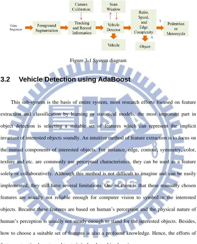
First of all, pre-processing module straightly uses the raw data of surveillance video as inputs. We transform the raw color image into a gray level image, for acceleration, the gray level image is downsized by a simple down-sampling algorithm. After resizing, the image is send to Gaussian mixture model (GMM) approach to obtain reliable background images, and then use background subtraction technique to extract foreground objects. In this stage, we use calibration for transferring pixel coordinates to world coordinates and cooperate with foreground subtracted by GMM to get and record foreground’s information, such as width, height, and speed for further classification. Here, we use concept of overlapping area for tracking and recording foreground’s information. For classification’s criteria, the AdaBoost vehicle detector uses slicing window to detect vehicles and verifies whether the foreground subtracted by GMM is vehicle. Through AdaBoost vehicle detector, we can separate vehicles from motorcycles, pedestrians and objects. Next, we utilize width and height ratio, speed get from calibration, and edge complexity to separate pedestrians and objects. Because we found that pedestrians and objects have different edge complexity range.

Figure 3-1 System diagram

3.2

Vehicle Detection using AdaBoost

This sub-system is the basis of entire system, most research efforts focused on feature extraction and classification by learning or statistical models, the most important part in object detection is selecting a suitable set of features which can represent the implicit invariant of interested objects soundly. An intuitive method of feature extraction is to focus on the mutual components of interested objects. For instance, edge, contour, symmetry, color, texture and etc. are commonly use perceptual characteristics, they can be used as a feature solely or collaboratively. Although this method is not difficult to imagine and can be easily implemented, they still have several limitations. One of them is that these manually chosen features are usually not reliable enough for computer vision to symbolize the interested objects. Because these features are based on human’s perception and the physical nature of human’s perception is usually not steady enough to stand for the interested objects. Besides, how to choose a suitable set of features is also a profound knowledge. Hence, the efforts of feature extraction have turned to statistical and machine learning areas.

AdaBoost algorithm proposed by Y. Freund et al. [1] is one of machine learning techniques and has been widely used for pattern recognition and progressed rapidly. AdaBoost algorithm combines weak classifiers into a strong classifier by weighted voting machine, and it shows high performance in diverse fields. P. Viola et al [2] used AdaBoost

algorithm to build an efficient pedestrian detector, which has trained a series of progressively complex rejecting rules based on Haar-like wavelets and space-time differences. In P. Viola, M. J. Jones [3], AdaBoost algorithm is applied to face detection and yields the best performance comparable to the previous researches. Like previous concept, we want to build a vehicle detector using several features that can stand for vehicles. Therefore, we adopt Haar-like features, which will be described in section 3.2.1. In order to build a vehicle detector, we use AdaBoost algorithm to select useful Haar-like features and combine them into a strong classifier, which will be explained in details in section 3.2.3.

3.2.1 Haar Features (Rectangle Features)

Haar basis functions (Haar-like features) used by Papageorgiou et al. [4] provide information about the grey-level intensity distribution of adjacent regions in an image. To compute the output of a Haar-like feature on a certain region of gray-level image, the sum of all pixels intensity in the black region is subtracted from the sum of all pixels intensity in the white one. To prevent square measures of white and black regions are different, the sums of black and white region are normalized by a coefficient. Figure 3-2 shows the set of Haar-like features, including primary and extended features. These features consist of two to four rectangles. P. Viola et al. [6] introduced the integral image to reduce computation time for the filters, which is an intermediate representation for an input image. The concept of integral image is illustrated in Figure 3-3(a), the value of the integral image at point (x, y) is the sum of all the pixels above and to the left. In Figure 3-3(b), the sum of the pixels within rectangle D can be computed with four array references. The value of the integral image at location 1 is the sum of the pixels in rectangle A. The value at location 2 is A + B, at location 3 is A + C, and at location 4 is A + B + C + D. The sum within D can be computed as 4 + 1 − (2 + 3). Utilizing integral images, sum of a rectangular region can be calculated by using only four

can be computed by using only six references in the integral image, eight in the case of the three-rectangle Haar features, and nine for four-rectangle filters.

Every Haar feature j is defined as fj(rj, wj, hj, xj, yj), where rj is the type of Haar feature,

wj and hj are width and height of the Haar feature and (xj, yj) is its position in the window. ) , , , , (r w h x y f

valuesubtracted , is the weighted sum of the pixels in white rectangles subtracted

from those of black rectangles.

Figure 3-2 The Haar-like features [5]

3.2.2 Weak Classifier

A weak classifier h is composed of a Haar-like feature f (defined in 3.2.1), a threshold (θ) and a polarity (p) indicating the direction of the inequality in Equation 3-1.

     otherwise p f p if h j j j j 0 1  (3-1) Here fj is the absolute value of the Haar feature j, θj is the threshold, and pj is the parity.

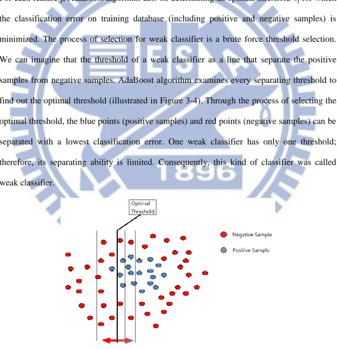
For each feature j, AdaBoost algorithm acts on determining an optimal threshold θj for which

the classification error on training database (including positive and negative samples) is minimized. The process of selection for weak classifier is a brute force threshold selection. We can imagine that the threshold of a weak classifier as a line that separate the positive samples from negative samples. AdaBoost algorithm examines every separating threshold to find out the optimal threshold (illustrated in Figure 3-4). Through the process of selecting the optimal threshold, the blue points (positive samples) and red points (negative samples) can be separated with a lowest classification error. One weak classifier has only one threshold; therefore, its separating ability is limited. Consequently, this kind of classifier was called weak classifier.

3.2.3 AdaBoost Algorithm

There are different methods have been used for features selection in literature. For instance, Principal Component Analysis (PCA) used in [7, 8, 9], Independent Component Analysis (ICA) used in [10] and so forth. Compared with those algorithms, AdaBoost has shown its capability to improve the performance of selecting features and increase the detection rate.

As mentioned before(section 3.2.1), the feature set came from the permutation of Haar-like feature types, scales and positions , is many times larger than the number of pixels in the input image. Even through each rectangle feature can be computed by integral image efficiently, computing the complete set is still extremely time consuming. AdaBoost algorithm uses the feature set to select weak classifier and combines several weak classifiers into a strong classifier defined in Equation 3-2. Those weak classifiers selected by this iterative algorithm have moderate discrimination and precision.

    _ 





Consider a 2D feature space containing positive and negative training samples.A weak classifier needs only do better than chance, namely separates the training samples with at least 50% accuracy. At beginning, AdaBoost will select a weak classifier with the highest accuracy in current training round to separate the training samples by its optimal threshold. As shown in Figure 3-5(b) and Figure 3-5(d), samples misclassified by a previous weak classifier are given more stress at future rounds. The training process will focus on these misclassified and difficult samples through increasing weights, which cannot be correctly separated by single

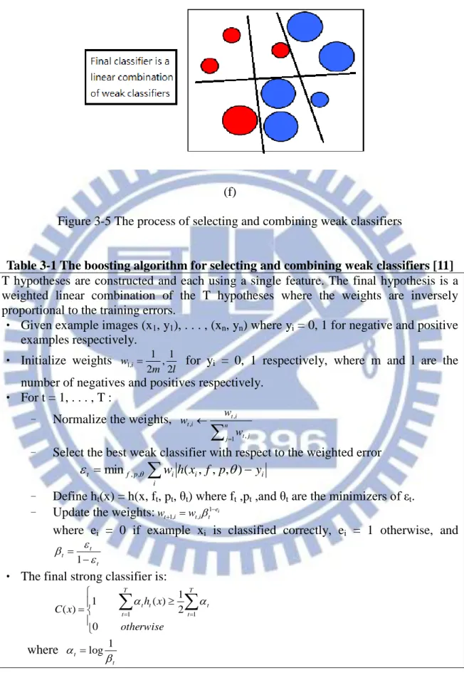
weak classifier. The concept and process of how AdaBoost selects weak classifiers and combines them into a strong classifier is shown in Figure 3-5(a)(b)(c)(d)(e)(f). As shown in Figure 3-5(a), the misclassified blue points (positive samples) in the upper side of the black line and red points (negative samples) in the downside of the black line are emphasized in the next round shown in Figure 3-5(b); similarly, the misclassified blue points in left side of the black line are emphasized in the next round, as shown in Figure 3-5(c) and Figure 3-5(d). Finally, the strong classifier is composed of a linear combination of weak classifiers shown in Figure 3-5(f), and the boosting algorithm for selecting a set of weak classifiers to form a strong classifier is shown in Table 3-1.

(a)

(c)

(d)

(f)

Figure 3-5 The process of selecting and combining weak classifiers

Table 3-1 The boosting algorithm for selecting and combining weak classifiers [11]

T hypotheses are constructed and each using a single feature. The final hypothesis is a weighted linear combination of the T hypotheses where the weights are inversely proportional to the training errors.

• Given example images (x1, y1), . . . , (xn, yn) where yi = 0, 1 for negative and positive

examples respectively. • Initialize weights l m wi 2 1 , 2 1 ,

1  for yi = 0, 1 respectively, where m and l are the

number of negatives and positives respectively. • For t = 1, . . . , T :

– Normalize the weights,



– Select the best weak classifier with respect to the weighted error



– Define ht(x) = h(x, ft, pt, θt) where ft ,pt ,and θt are the minimizers of εt.

– Update the weights: ei

t i t i t w w1,  ,1

where ei = 0 if example xi is classified correctly, ei = 1 otherwise, and

t t t _     1

• The final strong classifier is:

      





3.2.4 Cascaded Classifier

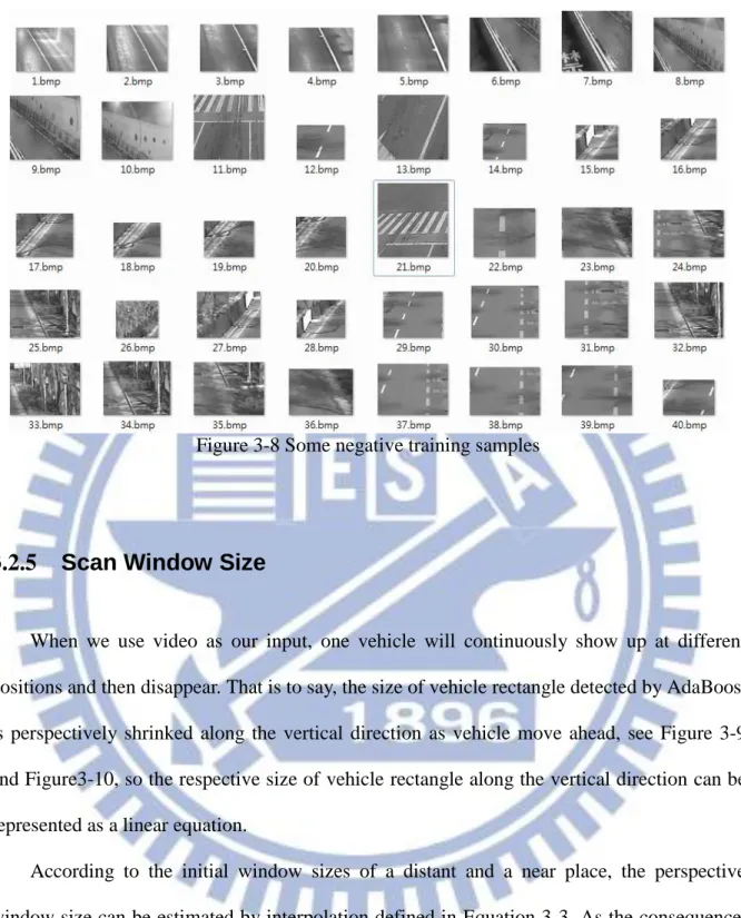
A cascaded classifier is constructed by stages of strong classifiers, and strong classifier is a stage composed of at least one weak classifier. P. Viola et al [3] proposed a cascading algorithm of AdaBoost described in Table 3-2. At each stage, if an object extracted by the searching window is classified as vehicle, it is permitted to enter the next stage; otherwise, the object is rejected immediately. In conclusion, an object needs to pass through a series of stages to be labeled as vehicle; otherwise, it is rejected by any stage even if it enters the last stage. Figure 3-6 demonstrates the structure of cascaded classifier. Figures 3-7 (a) to (c) are some positive samples we collect, including sedan, SUV, truck, and bus; and Figure 3-8 is some samples of negative samples.

Table 3-2 The training algorithm for building a cascaded detector[11].

• User selects values for f, the maximum acceptable false positive rate per layer and d, the minimum acceptable detection rate per layer.

• User selects target overall false positive rate, Ftarget.

• P = set of positive examples • N = set of negative examples

• F0 = 1.0; D0 = 1.0 • i = 0 • while Fi > Ftarget – i ← i + 1 – ni = 0; Fi = Fi-1 – while Fi > f × Fi-1 * ni ← ni + 1

* Use P and N to train a classifier with ni features using AdaBoost

* Evaluate current cascaded classifier on validation set to determine

Fi and Di.

* Decrease threshold for the ith classifier until the current cascaded

classifier has a detection rate of at least d × Di-1 (this also affects

Fi)

– N ← 0

– If Fi > Ftarget then evaluate the current cascaded detector on the set of

Figure 3-6 Structure of detection cascade

(b)

(c)

Figure 3-8 Some negative training samples

3.2.5 Scan Window Size

When we use video as our input, one vehicle will continuously show up at different positions and then disappear. That is to say, the size of vehicle rectangle detected by AdaBoost is perspectively shrinked along the vertical direction as vehicle move ahead, see Figure 3-9 and Figure3-10, so the respective size of vehicle rectangle along the vertical direction can be represented as a linear equation.

According to the initial window sizes of a distant and a near place, the perspective window size can be estimated by interpolation defined in Equation 3-3. As the consequence, we can calculate the scan window size at different vertical levels in advance. By utilizing this property, we can save a lot of time while using AdaBoost for vehicle detection.

Figure 3-9 As vehicles continuously move, the size of vehicle is perspectively shrinked.

Figure 3-10 Width of vehicle at different position

0 1 0 0 1 0 0 1 0 h h h h w w w w y y y y_{t t t}         (3-3)

3.3

Calibration Algorithm

3.3.1 Concept of Calibration

Most calibration methods [12]-[15] use known features in a scene to evaluate the camera parameters, including tilt angle, pan angle, and focal length. In [16] and [17], sets of parallel lines of a hexagon are utilized to calculate the camera parameters. Results from these papers show that parallel lines can be used to appropriately determine the camera parameters. Efficient algorithms [18]-[20] have been developed for evaluating the camera parameters utilizing parallel lanes in a traffic scene. In [18], the authors took advantage of the height and the tilt of the camera together with a pair of parallel lines in a traffic scene to calibrate the camera. Nevertheless, their method needs particular manual operations to measure the tilt angle of the camera. Multiple parallel lanes and a particular perpendicular line were used to calibrate the camera parameters in [19] and [20].

In this paper, a novel equation will be derived to calculate the vanishing point from two line we give in pixel coordinate. The derivation requires only a single set of parallel line, the reference width, and the reference height. Compare the proposed method with the existing approaches and we’ll see our method has the advantage of requiring neither the camera’s information nor multiple sets of parallel lines. The purpose of using calibration in this paper is to transform the pixel coordinates into their corresponding world coordinates. To get the width and height ratio in world coordinates, we first need to calibrate the pixel coordinates to obtain meaningful results. For example, the accuracy of comparing speed and length ratio of motorcycles, pedestrians, and objects depends on the accuracy of calibration’s results.

3.3.2 Proposed Calibration Method

The purpose of calibration is to determine the required parameters for estimating the world coordinates from the pixel coordinates of two given points in an image frame; that is to say, through calibration we can transform a period of length in pixel coordinates to world coordinates to get its real length in world. This section will be organized as follows: firstly, we will show the flow chart of calibration; secondly, we will present the function of creating line and the derivation of vanishing point; finally, we will demonstrate the derivation of transforming a period of length in pixel coordinates to world coordinates.

Function of creating line

We need two points to get a straight line. Using the following mathematical formulas, one can transform the two points we get into their corresponding straight line.

We name the two points as (x1,y1)and (x2,y2), line function as axbyc0. Then we can get “a” asy2 y1, “b” as (x2x1), “c” as x1ay1b.

Vanishing point

After the two lines have been calculated, we can take advantage of the two lines to estimate vanishing point. We name the parameters of left side of line we get as L.a, L.b,

c

L. , and the parameters of right side of line we get as R.a, R.b, R.c. If temporary _value

=R.aL.bL.aR.b is not equivalent to zero, namely left line and right line are parallel, then we can get vanishing point (u0,v0) as Equation(3-4) and Equation (3-5)

value temporary c L b R c R b L u0(( .  . )( .  . ))/ _ (3-4) value temporary c L a R c R a L v0( .  .  .  . )/ _ (3-5)

Some parameters

We define the square of reference width as l1 and square of reference height as l2 and image canter as(cu,cv). Then we can get parameters cX and cY as follows equations:

) 1 2 2 1 /( ) 1 2 2 1 (l b l b a b a b cX        (3-6) ) 1 2 2 1 /( ) 1 2 2 1 (l a l a b a b a cY       (3-7) Here a1, a2, b1, and b2 are transformed from the eight points we give, namely two parallel line, one reference width, and one reference height.

After calibrating, we can transform length in pixel-based coordinates system to world coordinates system as follows:

) _ 0 /( 0 ) _ ( 0 cX start x cu v v cv start y w       (3-8) ) _ 0 /( 0 ) _ ( 1 cY cv start y v v cv start y w       (3-9) ) _ 0 /( 0 ) _ ( 2 cX end x cu v v cv end y w       (3-10) ) _ 0 /( 0 ) _ ( 3 cY cv end y v v cv end y w       (3-11) 2 2 ) 1 3 ( ) 0 2 (w w w w length    (3-12) Here we define the length, namely the two points given in pixel coordinates

) _ , _

(start x start y and (end_x,end_y), which will be transformed to world coordinates geting the real length.

3.4

Classification

3.4.1 Method of Recording Foreground’s Information

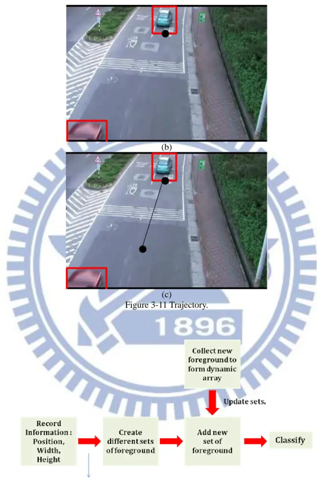
The purpose of tracking and recording foreground’s information is for further classification. As vehicles, motorcycles, or pedestrians are continuously moving, the consecutive foreground’s rectangles of the same vehicle, motorcycle, or pedestrian will overlap. We exploit the principle of overlapping area of detected foreground rectangles will reach a certain amount for tracking. We take advantage of tracking’s result of the foreground’s trajectory and FPS to calculate its speed. That is to say, we need distance and time to get foreground’s speed. We use trajectory and calibrate it to get distance, as shown in Figures 3-11(a) to (c). For each foreground, we will record its position, width, and height of the world coordinates which gets from calibration. Then, we use the concept of overlapping area to create different sets of them for further classification. When we find that there is an foreground that does not belong to any of the collection which is already recorded, we will update the sets. That is to say, we will add an new set for the new foreground for further classification. Figure 3-12 is the diagram of recording foreground’s information.

(b)

(c)

Figure 3-11 Trajectory.

3.4.2 Edge Complexity

There are some features can be used to describe objects. For examples, Luo-Wei Tsai et al [27] used color, edge and corner to identify vehicles in the static image and A. Kuehnle et al [28] used the symmetry of edge as features of vehicles. In this study, we do not consider using color as one of the features to do classification because in the pre-processing stage we transform the input frame to gray-level image for further use and the Haar-like features used in AdaBoost algorithm are also operating on gray-level image. In other words, the AdaBoost vehicle detector we trained uses only gray-level information. Furthermore, we do not use corner to separate objects and pedestrians. It is hard to discriminate pedestrians from objects by using corner only, because there are too many objects have similar corner as pedestrians. As the consequence, it is hard to separate the pedestrians efficiently from the objects by using the number of corners on them or the position information of corners. In our classification’s criteria, we chose edge as the main feature and use edge complexity [29] to classify objects and pedestrians. First, we use Canny operator [30] to obtain the edge image of each object and pedestrian candidates. Figure 3-13 is some edge image examples. We do not use the whole frame to compute the edge complexity; instead, we just utilize the foreground get from previous stage to acquire the edge image. It is because that use the whole frame to compute edge is time-consuming. Besides, the purpose of using edge complexity is to separate objects and pedestrians. Therefore, we just look at the candidates of objects and pedestrians and compute their edge complexity here by Equation 3-13.

(3-13) Here mc is the edge complexity, is the number of edge pixel and n is the number of pixel. We found that objects and pedestrians have different edge complexity range as defined in Equation 3-14, namely pedestrians’ edge complexity is larger than objects’.





c

m (3-14) Here  is an empirical threshold for the purpose of classify objects and pedestrians. By using edge complexity, the system can do classification completely.

Figure 3-13 Some examples of edge image

3.4.3 Classification Criteria

Our aim is to classify vehicles, pedestrians, and objects. We view vehicles which includes sedan, SUV, truck, and bus as the same class; and motorcycles, pedestrians as the same class. First, we employ GMM to get foreground and record foreground’s width, height, and speed get from calibration. The classification method can be divided into two stage, as shown in Figure 3-14. In first stage, we take advantage of AdaBoost to detect vehicles which separates vehicles from pedestrians, motorcycles, and objects. In second stage, we discovered that pedestrians, motorcycles, and objects have different edge complexity range, which th2 is empirical threshold. Therefore, we use edge complexity cooperates with width and height ratio which th1 is empirical threshold, and speed which contains distance get from calibration and time get from FPS(namely frame per second) to separate pedestrians, motorcycles from objects.

Chapter 4 Experimental Results

The proposed system is implemented on a PC system. The CPU and RAM of the PC is Intel(R) Core(TM) i5-2410M CPU @ 2.30GHz and 8GB RAM respectively.

The integrated development environment is Microsoft Visual Studio 2008 on Windows 7. The inputs are video files (uncompressed AVI). These inputs were captured with a DV at various traffic scenes.

Section 4.1 illustrates the training process of AdaBoost, including the training dataset and the criterion of collected samples. Section 4.2 demonstrates the experimental results of detecting vehicles in videos. Section 4.3 illustrates the experimental results of classification in videos.

4.1

AdaBoost Training

Part of the proposed system based on machine learning algorithm which involves training processes and testing processes. Sample collection is the key of object detection. To build the AdaBoost vehicle detection system, first, the common components of vehicles must be determined (e.g., lamps, wheels, bumper ... etc.), the foundation of collecting samples is keeping these common parts and eliminating unnecessary parts to reduce the interference of noise; therefore, the images are tightly cropped. Second, the manually collected samples are usually not uniform in size, because of some conditions, like illumination, a normalization process is necessary, so that the positive samples is normalized before entering training or testing step.

The study takes advantage of AdaBoost vehicle detection system for further application. The proposed system presently focuses on rear views of vehicles such as sedans, sport-utility vehicles (SUVs), minivans, and trucks which are the majority of traffic. The collected samples

of proprietary database were cut out from proprietary videos captured in daytime. The captured sources contain several scenes. While collecting vehicle samples, the pose of captured cars is restricted to rear-views and the angle tolerance of pan-rotation range is about ±20°. Figure 4-1 demonstrates the diagram of extracting samples from video frames.

Figure 4-1 Diagram of extracting vehicle samples

Lamps, wheels, bumper are the main characteristics chosen to recognize a vehicle in our proposed AdaBoost vehicle detection system. As a result, all manually cropped vehicle samples should contain these components without occlusion. In crowded scenes, a vehicle is sometimes occluded by other vehicles, so the following vehicle will not be a qualified sample until the preceding vehicle moves over. Accordingly, the sizes of extracted samples are inconsistent, we have to normalize those positive samples. We normalize the width and height of our collected 5354 vehicle samples to 24 x 16. Through normalization, the samples can be resized in an equivalent ratio, namely 3:2. Figures 4-2 (a) to (c) demonstrate some collected positive and negative samples and Figure 4-3 is the flow chart of the training process.

(a)

(c)

Figure 4-2 Some collected positive and negative samples

In this study, the raw input of AdaBoost training process is the gray level information of 5354 vehicle images and 12642 non-vehicle images from the proprietary database. The gray level information is normalized to a uniform size 24 x 16 without any further processing. The weak classifiers used here are the permutation of the type, position and scale of 15 Haar-like features. The scale of Haar features is increased in a brute force manner, i.e. the size of Haar features is from 2 x 2 to 24 x 16 progressively. The final classifier is a 17 layer cascade of classifiers which included a total of approximately 1000 weak classifiers.

In addition, while training AdaBoost vehicle detector, we use 0.996 and 0.48 for the minimum hit rate and maximum false alarm rate per layer respectively in our study.

4.2

Results of Detecting Vehicles in Video

In this section, the experimental results of detecting vehicles in videos are demonstrated. The testing videos are composed of lots of different scenes, like tunnel, outdoors, and roadway. Tables 4-1 to Table 4-2 are the statistic results of testing videos between different scenes and situations, such as vehicles with shadow and rainy day.

Table 4-1 Detection rate, false alarm, and FPS between different scenes

Setting Total Vehicles Detected vehicles False alarm FPS Shadow 295 290(98.3%) 3(1.02%) 27.56 Rainy+sway 20 19(95%) 2(9.52%) 23.11 Flyover 381 357(93.7%) 2(0.55%) 26.38

Table 4-2 Detection rate, false alarm, and FPS between different scenes

Setting Total Vehicles Detected vehicles False alarm FPS

Outdoors 35 35(100%) 0(0%) 25.64

Tunnel 217 205(94.47%) 6(2.84%) 27.71 Roadway 496 479(96.57%) 3(0.62%) 28.54 The criteria of performance measurement which includes detection rate and false alarm rate are defined in Equations 4-1 and 4-2 [9] respectively.

(4-1) (4-2) Here false alarm means detected amiss windows. As illustrated in Tables 4-1 to Table 4-2, the result is identical to our objective, namely can be applied to detect various kinds of back-viewed vehicles in a scene and real-time application.

Figures 4-4 (a) to (f) are some captured pictures of detection result corresponding to Table 4-1 to Table 4-2. The red rectangle is the result of proposed system.

(a)Tunnel

(b)Vehicle with shadow

(d)Outdoors

(e)Roadway

(f)Rainy+sway

Figure 4-4 Captured pictures of detection result

We also compared the result with J.F. Lee [31], namely AdaBoost using the whole front vehicle image as training samples+ Probabilistic Decision-Based Neural Network (PDBNN) and method which used Gaussian Mixture Model (GMM)[22][23] to establish background image. Table 4-3 is the statistic results of testing videos. We also present comparison of the frame per second (FPS).

Table 4-3 Performance comparison of video

Place Method Detected vehicles False alarms FPS Total vehicles 台中市

大墩路

GMM 110( 82.09% ) 7( 5.98% ) 20.74 134 AdaBoost + PDBNN[31] 131( 97.76% ) 2( 1.5% ) 7.44

Proposed system 132( 98.5% ) 2( 1.49% ) 18.32

In this table, both method in [31] and our proposed system perform well. As for GMM, because the scene we used has heavy traffic and contain vehicles and motorcycles in the same time, it is hard for GMM method to segment vehicle will and distinguish motorcycle from vehicle. As illustrated in Table 4-3, the result is identical to our objective, namely can be applied to real-time application.

Obviously, use the rump of vehicles as positive samples is better than using the entire vehicle. It is because of when we use the rump of vehicles as training database, we actually decreased the complexity of positive samples, namely the similarity of positive samples is higher than using the entire vehicle as training database.

4.3

Results of Classification in Video

In this section, the experimental results of classification in videos are demonstrated. For the testing videos, every single frame is treated as a static image, and the size of video frames will be normalized to 320 x 240. Before classification, we will go through the process of calibration in order to get the information in world coordinates to do classification. By calibrating, the pixel coordinates will be transformed to world coordinates. After calibrating, every single frame will go through the proposed system to do classification. Figures 4-5 (a) to (i) show the experimental results. The red rectangle represents the foreground is classified

into vehicle. The white rectangle represents the foreground is classified into pedestrian or motorcycle. The green rectangle represents the foreground is classified into object. The testing scene is in Hsichu, Guangfu Rd.

(a) (b)

(c) (d)

(g) (h)

(i)

Chapter 5 Conclusions and Future Work

The proposed classification system which includes AdaBoost vehicle detector and calibration method we proposed can do classification well. At AdaBoost vehicle detector stage, the prime priority is to detect and verify the foreground get from Gaussian Mixture Model whether is a vehicle. At the calibration stage, the top mission is to record the information of the extracted foreground, such as width and height in the world coordinates. At classification stage, we take advantage of AdaBoost vehicle detector and calibration’s result cooperate with edge complexity and width and height ratio to do classification. Each stage of system has its main functionality and can perform well when they are combined together. This paper demonstrates a robust system for vehicles, pedestrians, and objects classification which can operate well and can be applied to real-time applications. This paper also presents a robust vehicle detection system which can detect various kinds of back-viewed vehicles in a scene.

To further improve the performance of our system, some enhancements or trials can be made in the future, such as the performance might be further reinforced by adding auxiliary features. In addition, the proposed system can be developed to auto-calibration system, like including line-detection. Finally, the experimental results show the opportunity of classifying vehicles, like sedan, truck and bus or classifying pedestrians and motorcycles.

References

[1] Y. Freund and R. E. Schapire, “Experiments with a new boosting algorithm,” in Proceedings of the 13th International Conference on Machine Learning (ICML ’96), pp. 148–156, Bari, Italy, July 1996.

[2] P. Viola, M. J. Jones, and D. Snow, “Detecting pedestrians using patterns of motion and appearance.” The 9th ICCV, Nice, France, volume 1, pages 734–741, 2003.

[3] Paul Viola, Michael J. Jones “Robust Real-Time Face Detection” International Journal of Computer Vision 57(2), 137–154, 2004 Kluwer Academic Publishers.

[4] C. Papageorgiou, M. Oren, and T. Poggio "A general framework for object detection," International Conference on Computer Vision, 1998.

[5] Rainer Lienhart and Jochen Maydt, "An Extended Set of Haar-like Features for Rapid Object Detection," IEEE ICIP 2002, Vol. 1, pp. 900-903, Sep. 2002.

[6] Paul Viola, Michael J. Jones “Robust Real-Time Face Detection” International Journal of Computer Vision 57(2), 137–154, 2004 Kluwer Academic Publishers.

[7] J. Ferryman, A. Worrall, G. Sullivan, and K. Baker, “A Generic Deformable Model for Vehicle Recognition,” Proceedings of British Machine Vision Conference, pp. 127–136, 1995.

[8] Z. Sun, R. Miller, G. Bebis and D. Dimeo, “A Real-time Precrash Vehicle Detection System,” IEEE Intelligent Vehicles Symposium 2000. Dearborn, MI, USA.

[9] Chi-Chen Raxle Wang and Jenn-Jier James Lien “Automatic Vehicle Detection Using Local Features – A Statistical Approach” IEEE Transactions on Intelligent Transportation Systems, Vol. 9, No. 1, March 2008.

[10] Chris Harris and Mike Stephens, "A Combined Corner And Edge Detector", Forth Alvey Vision Conference, Manchester, UK, pp147-151

NCTU, JULY, 2010

[12] A. M. Sabatini, V. Genovese, and E. S. Maini, “Toward low-cost vision-based 2D localisation systems for applications in rehabilitation robotics,”in Proc. IEEE Int. Conf. Intell. Robots Syst., Lausanne, Switzerland, 2002,pp. 1355–1360.

[13] F.-Y. Wang, “A simple and analytical procedure for calibrating extrinsic camera parameters,” IEEE Trans. Robot. Autom., vol. 20, no. 1,pp. 121–124, Feb. 2004.

[14] S. Ying and G. W. Boon, “Camera self-calibration from video sequences with changing focal length,” in Proc. IEEE Int. Conf. Image Process.,Chicago, IL, 1998, vol. 2, pp. 176–180.

[15] E. Izquierdo, “Efficient and accurate image based camera registration,”IEEE Trans. Multimedia, vol. 5, no. 3, pp. 293–302, Sep. 2003.

[16] T. Echigo, “A camera calibration technique using three sets of parallellines,” Mach. Vis. Appl., vol. 3, no. 3, pp. 159–167, Mar. 1990.

[17] L.-L. Wang and W.-H. Tsai, “Camera calibration by vanishing lines for 3-D computer vision,” IEEE Trans. Pattern Anal. Mach. Intell., vol. 13,no. 4, pp. 370–376, Apr. 1991. [18] E. K. Bas and J. D. Crisman, “An easy to install camera calibration for traffic

monitoring,” in Proc. IEEE Conf. Intell. Transp. Syst., Boston,MA, 1997, pp. 362–366. [19] C. Zhaoxue and S. Pengfei, “Efficient method for camera calibrationin traffic scenes,”

IEE Electron. Lett., vol. 40, no. 6, pp. 368–369,Mar. 2004.

[20] A. H. S. Lai and N. H. C. Yung, “Lane detection by orientation andlength discrimination,” IEEE Trans. Syst., Man, Cybern. B, Cybern.,vol. 30, no. 4, pp. 539–548, Aug. 2000. [21] Lisa M. Brown, “View independent vehicle/person classification,”in Proceedings of

the ACM 2nd international workshop on Video surveillance and sensor networks, 2004, pp. 114–123.

tracking", IEEE Computer Society Conference on Computer Vision and Pattern Recognition, 1999., vol.2, no., pp.-252 Vol. 2, 1999.

[23] Peng S., Yanjiang W.,“An improved adaptive background modeling algorithm based on Gaussian Mixture Model”, Signal Processing, 2008. ICSP 2008. 9th International Conference, pp. 1436-1439, 26-29 Oct. 2008.

[24] www.vision.caltech.edu/bougueti/calib doc/

[25] C. Papageorgiou and T. Poggio, “A trainable system for object detection,” International Journal of Computer Vision, vol. 38, no. 1, pp. 15–33, 2000.

[26] Pablo Negri, Xavier Clady, Shehzad Muhammad Hanif, and Lionel Prevost “A Cascade of Boosted Generative and Discriminative Classifiers for Vehicle Detection” EURASIP Journal on Advances in Signal Processing Volume 2008, Article ID 782432, 12 pages.

[27] Luo-Wei Tsai, Jun-Wei Hsieh and Kuo-Chin Fan, "Vehicle Detection Using Normalized Color and Edge Map", IEEE Transactions on Image Processing, Vol. 16, No.3 MARCH, 2007.

[28] A. Kuehnle, “Symmetry-based recognition of vehicle rears,” Pattern Recognit. Lett., vol. 12, no. 4, pp. 249–258, Apr. 1991.

[29] Wen-Chung Chang and Chih-Wei Cho, "Online Boosting for Vehicle Detection", IEEE Transactions on Systems, Man, and Cybernetics-PART B:Cybernetics, Vol. 40, No.3 JUNE. 2010.

[30] Chris Harris and Mike Stephens, "A Combined Corner And Edge Detector", Forth Alvey Vision Conference, Manchester, UK, pp147-151

[31] Ja-Fan Lee,"A Novel Vehicle Detection System Using Local and Global Features", NCTU, JULY, 2010