用於行動照護應用之低能量同步非同步混合式心電訊號特徵擷取器設計

國

立

交

通

大

學

電子工程學系 電子研究所

碩 士 論 文

用於行動照護應用之低能量同步非同步混合式

心電訊號特徵擷取器設計

An Energy-Efficient

Mixed Sync-Async Cardiac Delineator

for Mobile Healthcare Applications

研 究 生：張博堯

指導教授：李鎮宜 教授

用於行動照護應用之低能量同步非同步混合式

心電訊號特徵擷取器設計

An Energy-Efficient

Mixed Sync-Async Cardiac Delineator

for Mobile Healthcare Applications

研 究 生： 張博堯 Student：Po-Yao Chang

指導教授： 李鎮宜 Advisor：Chen-Yi Lee

國 立 交 通 大 學

電子工程學系 電子研究所

碩 士 論 文

A Thesis

Submitted to Department of Electronics Engineering and Institute of Electronics

College of Electrical and Computer Engineering National Chiao Tung University

in partial Fulfillment of the Requirements for the Degree of

Master of Science in

Electronics Engineering

January 2013

Hsinchu, Taiwan, Republic of China

I

用於行動照護應用之

低能量同步非同步混合式心電訊號特徵擷

取器設計

學生：張博堯 指導教授：李鎮宜 博士

國立交通大學

電子工程學系 電子研究所

摘要

行動照護應用使用了具備無線傳輸能力的感測器來達到生理狀況監控，能夠 長時間的監控就成為了這類應用的主要需求。我們藉由在感測器上做訊號處理以 減少無線傳輸的資料量。在感測器上做事先的特徵擷取，傳輸的資料將可以被大 大地減少，同時擷取出的生理特徵也可被用於即時的疾病診斷，減少感測器到醫 院的診斷延遲時間，給予病患更大的保護。 以心血管疾病為例，心臟疾病的診斷是藉由心電圖的 P、Q、R、S、T 等特徵 的大小及區間來判斷。在這份論文中，我們提出了一個基於小波轉換的心電訊號 特徵擷取演算法及硬體，並且使用兩個標準的心電圖資料庫來驗證特徵擷取的結 果。我們提出的演算法對所有提供的特徵都達到了 99.4%及 96.1%以上的靈敏度 及準確率。在硬體架構上，擷取器被計在極低的操作頻率（250Hz），並藉由共 用搜尋核心、記憶體最佳化、以及觸發式的獨立電源管理非同步搜尋核心，來達 到低能量消耗的需求。極低的操作頻率加上非同步電路更提供了降低工作電壓來 降低功率消耗的可能性。我們提出的心電訊號擷取器採用 90 奈米標準 CMOS 製 成晶片實現。在 0.5V 的電源供應之下，擷取器功率消耗為 2.56 。最後，我們

II

也利用了市售晶片以及嵌入式處理器建構了一個極小的無線傳輸感測器模組來 驗證我們的特徵擷取演算法。藉由這個感測器模組，我們驗證了演算法的行動環 境中的準確率以及藉由特徵擷取減少資料傳輸能量的想法。

III

An Energy-Efficient

Mixed Sync-Async Cardiac Delineator for

Mobile Healthcare Applications

Student: Po-Yao Chang Advisor: Chen-Yi Lee

Department of electronics engineering and Institute of electronics,

National Chiao Tung University

Abstract

Long-term monitoring is the key requirements for mobile healthcare applications, where the wireless sensor nodes are worn to record the human’s vital signals. On-sensor signal analysis is proposed for these applications to enable timely detection of risky syndromes and extend the monitoring time. Instead of raw data transmission, the wireless transmission energy is reduced by only transmitting the vital features.

In case of cardiac diseases, the syndrome analysis is performed based on different extracted features of ECG signals like P, QRSon, R, QRSend, and T wave. In this work, an energy-efficient cardiac delineation algorithm based on multi-scale wavelet transform is designed together with its hardware implementation. The detection result is evaluated on two annotated databases including MIT-BIH arrhythmia database and QT database. The obtained sensitivity and positive predictivity are over 99.4% and 96.1% for the five ECG features, respectively. With shared search kernels, storage optimization and event-driven asynchronous search kernel with individual power management, the delineator can operate at 250Hz without the needs for additional high speed clock. The slow operating speed and asynchronous search kernel also enables further voltage scaling to reduce power. Implemented using UMC 90nm technology

IV

and operating at 250Hz with 0.5V supply voltage, the overall power is 2.56μW for real-time ECG monitoring.

Besides, a miniaturized prototype wireless sensor is constructed using commercial products with on-sensor delineation. The prototype provides evidence to the delineation robustness for mobile monitoring and power reduction for on-sensor feature extraction.

V

誌謝

很高興能夠在 Si2 實驗室完成我的碩士學歷。 感謝李鎮宜老師從我專題到研究所以來，給予我在研究以及人生上的指導。 實驗室完整的資源以及實力堅強的研究陣容讓我們在研究上能夠自由的發展。也 感謝口試委員黃威教授及莊景德教授，能撥空來指導並且給予我一些研究方面的 建議，使得本篇論文可以更加完整。 感謝在我的研究中一路給我指導的書餘學長，一路給我指導方和拉拔，讓我 能夠順利完成碩士學位。也感謝所有 Si2 實驗室的夥伴們以及所有電工系及熱舞 社的同學朋友，豐富了我在交大的生活。 最後感謝我的父母，謝謝你們從小的拉拔，沒有你們就沒有今天的我。謝謝 姊姊，從小到大一直包容我，我很想你，我愛你們。

VI

Table of Contents

Pages

Chapter 1: Introduction and Motivation ... 1

1-1 Introduction to Mobile Healthcare Application ... 1

1-2 Motivation ... 2

1-3 Introduction to Cardiac Signal ... 4

1-4 Organizations ... 9

Chapter 2: ECG Delineation Algorithm ... 10

2-1 Background ... 10

2-2 Dyadic Wavelet Transform (DWT) ... 12

2-2.1 Wavelet Theory ... 12

2-2.2 Quadratic Spline Wavelet Transform (QSWT) ... 14

2-3 Detection Algorithm ... 16

2-3.1 Wave Characteristic and Detection Flow ... 16

2-3.2 R Peak Detection ... 19

2-3.3 QRSon/end Detection ... 20

2-3.4 P/T Wave Detection ... 21

2-3.5 Adaptive Threshold and Window Update ... 22

2-4 Simulation Result and Performance Evaluation ... 24

2-5 Summary ... 28

Chapter 3: Asynchronous Design ... 29

3-1 Motivation ... 29

3-2 Introduction to Asynchronous Circuit ... 30

3-2.1 Moving from Synchronous to Asynchronous Approach ... 30

VII

3-2.3 Muller C Element ... 34

3-2.4 Asynchronous Pipelines ... 35

3-3 Design Flow Using Commercial CAD Tool ... 37

3-3.1 Design flow ... 37

3-3.2 Delay Margin Tuning ... 40

3-4 Design Example: An 16-tap FIR Filter ... 44

3-4.1 Iterative FIR Architecture and Implementation ... 44

3-4.2 Performance Comparison ... 47

3-5 Summary ... 51

Chapter 4: Architecture Design and Hardware Implementation ... 52

4-1 Architecture ... 52

4-2 Implementation Result ... 57

4-3 Comparison with State-of-The-Art ... 59

Chapter 5: Prototype Construction ... 60

5-1 Experiment Platform and System ... 60

5-2 On-Sensor ECG Delineator ... 61

5-3 Emulation Result ... 64

Chapter 6: Conclusion and Future Work ... 66

6-1 Conclusion ... 66

6-2 Future Work ... 67 Reference 68

VIII

List of Figures

Fig. 1-1 Scenario for mobile healthcare application... 1

Fig. 1-2 On-sensor delineation reduces Tx energy and provides real-time alarm ... 2

Fig. 1-3 The basic heart model and feautre waves inside a cardiac cycle ... 5

Fig. 1-4 P wave generation. ... 6

Fig. 1-5 AV node – the conduction blockage between atrial and ventricular. ... 7

Fig. 1-6 Ventricular contractionresulting in QRS complex ... 8

Fig. 1-7 The repolarization of ventricular results in T wave ... 8

Fig. 2-1 Morphological changes ECG signals extracted from QT database. ... 11

Fig. 2-2 (a) Mallat’s Algorithm, (b) algorithm á trous (SWT) ... 14

Fig. 2-3 A general ECG signal and the corresponded frequency response... 15

Fig. 2-4 The first 5 wavelet decomposition of ECG signal with noise coupling ... 17

Fig. 2-5 Flow graph for the proposed detection algorithm ... 18

Fig. 2-6 R peak detection detail ... 19

Fig. 2-7 QRSon/end detection detail ... 20

Fig. 2-8 Search window defined for P/T detection ... 21

Fig. 2-9 Detection result of ECGs with morphological changes and noise ... 24

Fig. 3-1 Delay variance under 1.0V and 0.5V supply voltage ... 29

Fig. 3-2 The difference between synchronous design and asynchronous design. ... 31

Fig. 3-3 (a) 4-phase handshake protocol (b) 2-phase handshake protocol ... 33

Fig. 3-4 Muller C element ... 34

Fig. 3-5 Fork and join structures ... 35

Fig. 3-6 Muller pipeline ... 35

Fig. 3-7 MOUSETRAP pipeline... 36

IX

Fig. 3-9 Break timing loops for un-constraint path ... 39

Fig. 3-10 Time constraints ... 40

Fig. 3-11 The delay distribution of datapath and delay line at different corner case ... 41

Fig. 3-12 Tuning Circuit including the tunable delay line and a lead-lag detector ... 42

Fig. 3-13 (a) The 8 tuning steps at 3 corners (b) Reduced margin ... 43

Fig. 3-14 Block diagram for the 16-tap FIR filter ... 44

Fig. 3-15 Ring structure for 4-pahse Muller pipeline ... 45

Fig. 3-16 The modified MOUSETRAP ring structure and time diagram ... 46

Fig. 3-17 Layout photo for the sync/async 16-tap FIR filter ... 47

Fig. 3-18 Energy distribution of the three asynchronous implementation ... 48

Fig. 3-19 Operation time/energy of the 3 async designs at corner and temperature .... 48

Fig. 3-20 Operation time/energy of sync/async design at different corners/temp. ... 50

Fig. 4-1 Delineator architecture ... 52

Fig. 4-2 The state transition graph of the QRS FSM. ... 53

Fig. 4-3 The architecture and pre-search process of QRSon ... 54

Fig. 4-4 The adaptive THR/WIN update engine ... 55

Fig. 4-5 Time diagram of the shared P/T search kernel ... 56

Fig. 4-6 The input and output interface for the asynchronous P/T kernel ... 57

Fig. 4-7 Power reduction with strategy at different design level ... 58

Fig. 4-8 Layout photo for the proposed cardiac delineator ... 58

Fig. 5-1 Experiment environment setup ... 60

Fig. 5-2 The prototype wireless sensor ... 61

Fig. 5-3 5 different Power mode supported by MPS430 micro-controller ... 62

Fig. 5-4 Delineation flow inside MSP430 ... 63

X

Fig. 5-6 SPI handshake protocol between MSP430 and G2 WIFI module ... 64 Fig. 5-7 User interface for real time display of ECG and extracted fiducial points ... 64 Fig. 5-8 Delineation Under mobile environment (with baseline drift) ... 65

XI

List of Tables

Table 1-1 Syndromes supported by the provided P, QRSon, R, QRSend, P features. ... 4 Table 2-1 R peak detection comparison with state-of-the-art detector using MITDB . 26 Table 2-2 Fiducial points delineation result comparison using QTDB ... 26 Table 2-3 R peak detection result within MITDB ... 27 Table 3-1 One encoding scheme for dual rail encoding ... 32 Table 3-2 CAD tools and design constraints used in the asynchronous design flow ... 37 Table 3-3 Energy distribution for the 3 asynchronous pipeline ... 48 Table 3-4 Comparison of the asynchronous and synchronous design at TT, 25°C ... 49 Table 4-1 Comparison of the proposed delineator with the state-of-the-art detector ... 59

1

Chapter 1:

Introduction and Motivation

1-1

Introduction to Mobile Healthcare Application

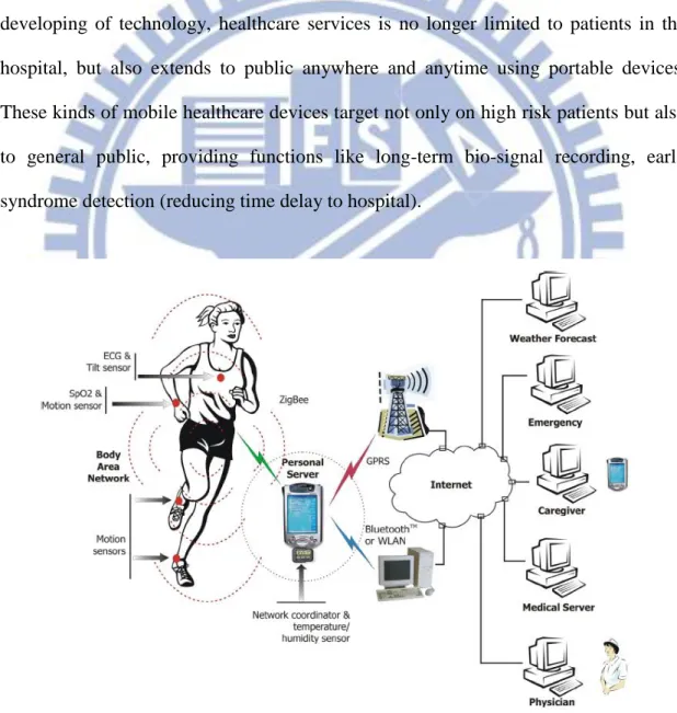
Mobile healthcare is defined broadly as the use of any mobile telecommunication technologies for the use of wireless health care delivery systems. Thanks to the developing of technology, healthcare services is no longer limited to patients in the hospital, but also extends to public anywhere and anytime using portable devices. These kinds of mobile healthcare devices target not only on high risk patients but also to general public, providing functions like long-term bio-signal recording, early syndrome detection (reducing time delay to hospital).

2

Fig. 1-1 shows the scenario of mobile healthcare. With different kinds of wireless sensor attached, information about body conditions such as ECG, EEG signals, blood pressures, and motion acceleration can be collected and transmitted through existed wireless connection to the hospital server for further data analysis.

1-2

Motivation

The challenge for these kinds of applications is the limited battery power for wireless sensor nodes. To extend monitoring time, many different kinds of technologies are proposed. Some aiming for more efficient wireless transmission, some emphasized on signal pre-processing on sensor nodes to reduce the transmission data by compression or feature extraction. Taking cardiac signal as example, feature extraction extracts the vital features that are required for syndrome diagnosis. With only the vital features transmitted, large transmission energy can be reduced. Besides, with the collected features, syndrome analysis can also be performed on the sensor for early alarm. Fig. 1-2 shows the possible implementation of such ECG processor.

Syndrome Classifier

Wireless Transmitter

Vital Features Extraction

Only vital features transmitted Real-time

Alarm

ECG Delineator Wireless Sensor Node

Fig. 1-2 By introducing on-sensor delineation, vital features can be extracted thus reducing transmission energy and providing real-time alarm to patients

3

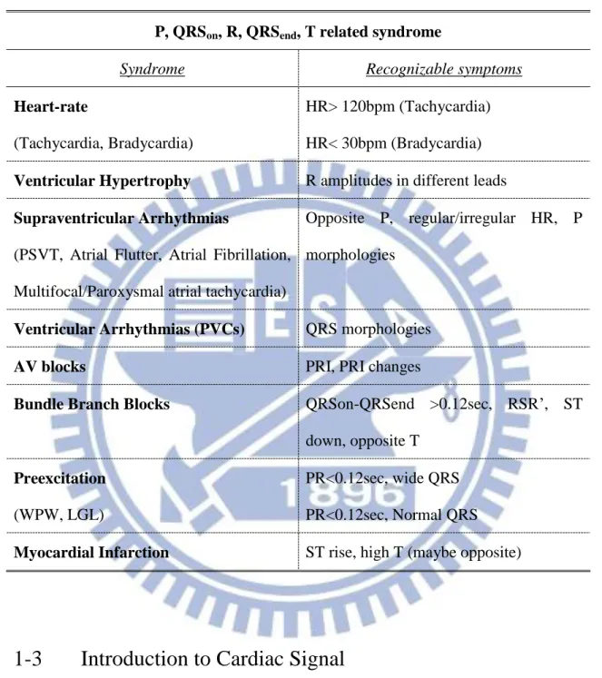
To satisfy the application requirement, low power and high accuracy feature extractor is required. There have been many algorithms proposed. However, most of them are designed for off-line detection, which are inappropriate for low power implementation [9] [10]. A real-time QRS detector has been implemented [14], nevertheless, the power is too large for mobile healthcare application (>100μW). Some low power hardware are proposed, but the detection accuracy is limited [16] or only the R peak is detected [16] [17] [18]. This limits the detection syndrome to only abnormal heart rate and confines the use for mobile healthcare applications. Therefore, we proposed a delineation algorithm with hardware implementation, which is able to detect the 5 most significant ECG features including P, QRSon, R, QRSend, and T wave. Table 1-1 lists the syndromes that can be detected with all 5 features. Various syndromes are supported, including high risk syndromes such as Myocardial Infarction, which cannot be detected by exist detectors.

To achieve further power reduction, the supply voltage for the delineator is scaled down. To combat the severe PVT variation under low supply voltage, we adopt asynchronous circuits to track the large delay variance for the critical design part. The most computation cost search P/T wave search kernel of the delineator is designed using a handshake template modified from the asynchronous 2-phase MOUSETRAP pipeline [21], while the rest part of the design can operate at low speed reducing the switching power. Because of the event-triggered property of P/T wave search, the search kernel can be power gated when idle. The use of asynchronous technique reduces the requirement for additional high speed clock source and exhibit fast power ON/OFF property suitable for such kind of design.

4

Table 1-1 Syndromes that can detected with the provided P, QRSon, R, QRSend, P features.

P, QRSon, R, QRSend, T related syndrome

Syndrome Recognizable symptoms

Heart-rate

(Tachycardia, Bradycardia)

HR> 120bpm (Tachycardia) HR< 30bpm (Bradycardia)

Ventricular Hypertrophy R amplitudes in different leads

Supraventricular Arrhythmias

(PSVT, Atrial Flutter, Atrial Fibrillation, Multifocal/Paroxysmal atrial tachycardia)

Opposite P, regular/irregular HR, P morphologies

Ventricular Arrhythmias (PVCs) QRS morphologies

AV blocks PRI, PRI changes

Bundle Branch Blocks QRSon-QRSend >0.12sec, RSR’, ST down, opposite T

Preexcitation

(WPW, LGL)

PR<0.12sec, wide QRS PR<0.12sec, Normal QRS

Myocardial Infarction ST rise, high T (maybe opposite)

1-3

Introduction to Cardiac Signal

This part introduces the basics of ECG signals. ECG is actually the voltage changes across the heart which can be measured by the sensor node attached to our skin. The basic waves in a cardiac cycle consist of the P, Q, R, S, and T waves. As the signals transmitted through the conducting cells triggering the myocardial cells according to all kinds of physical events, the voltage difference can be recorded and

5

analyzed. Fig. 1-3 (a) shows the basic waves of a general ECG in a cardiac cycle. Fig. 1-3 (b) shows a basic heart model including the conducting system. The mechanism of a heart beat is like this: the pacemaker cells (sinus node) perform the action of depolarizing and repolarizing at a certain frequency based on the status of sympathicus and the required amount of cardiac output. At every depolarizing and repolarizing, an action potential is generated, and this voltage change transmits to the myocardial cells through the help of the electrical conducing cells. Among receiving the depolarizing signal, Ca+ will be liberated into the myocardial cells resulting in contraction.

A general cardiac cycle consists of several wave characteristic as previously shown in Fig. 1-3 (a). . They are generated by electrical events such as:

 Atrial depolarization

 A pause separated the atria from the ventricles  Ventricular depolarization  Repolarization AV node Sinus node Ventricular Atrial Purkinje fibers P Q R S T PR interval QT interval PR segment QRS complex (a) (b) Ventricular Conducting system Atrial Conducting system

Fig. 1-3 (a) The basic waves inside a cardiac cycle. (b) A basic heart model including the conducting path

6

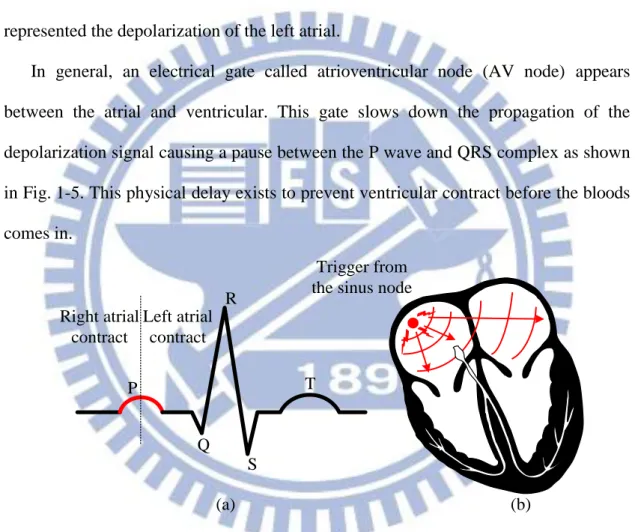
To begin, the activation of the sinus node generates a depolarization wave propagating to the myocardial cells of atrial, causing the atrial to contract. This event can be detected and is regarded as the P wave (Fig. 1-4). Because the sinus node is located at the right atrial, the right atrial will contract first. The first half of P wave is represented by the depolarization of the right atrial and the later part of P wave is represented the depolarization of the left atrial.

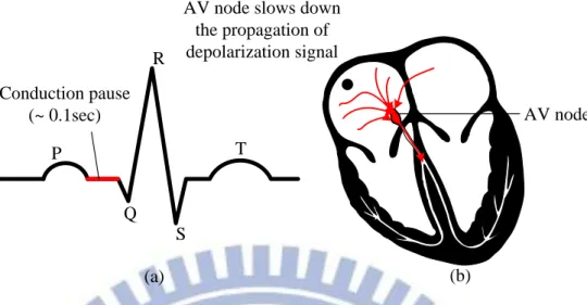
In general, an electrical gate called atrioventricular node (AV node) appears between the atrial and ventricular. This gate slows down the propagation of the depolarization signal causing a pause between the P wave and QRS complex as shown in Fig. 1-5. This physical delay exists to prevent ventricular contract before the bloods comes in. P Q R S T (a) (b) Right atrial contract Trigger from the sinus node Left atrial

contract

7 P Q R S T (a) (b) AV node AV node slows down

the propagation of depolarization signal Conduction pause

(~ 0.1sec)

Fig. 1-5 The AV node slows down the depolarization signal result in a small pause between the contraction of atrial and ventricular.

After about 0.1 seconds of delay, the depolarization wave propagates through the AV node along the Purkinje fibers causing the ventricular to contract. This physical event results in a new transition on ECG signal and is regarded as the QRS complex. Because ventricular is usually larger and the network of Purkinje fibers is more complex than atrial, the amplitude of QRS complex is larger and shape varying (Fig. 1-6).

After depolarization of all the cells, there will be a time interval where no more contraction can be made, called the refractory period. During this period, cells repolarized in order for the trigger of the next depolarization. This repolarization process of ventricular also results in a wave called T wave (Fig. 1-7). Note that the repolarization of atrial also generates a wave. But because it occurs at the same time as ventricular depolarized, the wave is covered by the QRS complex.

8 P Q R S T (a) (b) Ventricular contraction resulting in QRS complex

Fig. 1-6 Depolarization transmits through the Purkinje fibers causing ventricular to contract. The signal event showing on ECG is known as the QRS complex

P Q R S T (a) (b) Repolarization of ventricular resulting in T wave

9

1-4

Organizations

The thesis is organized as follows. Chapter 2 explains the proposed multi-scale wavelet-based delineation algorithm and the performance comparison with other existing algorithms verified using standard ECG databases. Chapter 3 presents the motivation for moving from synchronous to asynchronous circuit design. We first introduce the basics for asynchronous design. A 2-pahse handshake protocol targeting especially for iterative computation is proposed. A design flow for such asynchronous design using commercial CAD tools, together with an example design of 16-tap FIR filter is shown in this chapter. Chapter 4 describes the architecture and hardware implementation of the proposed mixed sync-async cardiac delineator with low power techniques at different design level. A prototype wireless sensor is constructed using embedded micro-controller with on-sensor delineation to verify the delineation for real mobile environment in chapter 5. Finally, chapter 6 gives the conclusion and future work.

10

Chapter 2:

ECG Delineation Algorithm

2-1

Background

ECG is the transthoracic interpretation of the electrical activity of heart over a period of time. A typical ECG tracing of the cardiac cycle (heartbeat) consists of a P wave, a QRS complex, and a T wave. The most commonly used features, which delineates the ECG waveform, are the signal amplitude and intervals within P, QRSon, R, QRSend, T wave boundaries.

The detection of these features is challenging for several reasons:

 Because of the small amplitude of ECG signal (<5mV), it is usually coupled with noise and artifacts, such as power line interference, electrode contact noise, patient-electrode motion artifacts, Electromyography (EMG), baseline wandering, data collecting device noise, quantization noise and aliasing, etc.  The wide variation of QRS morphologies and rhythms, from abnormal ECGs

and interpersonal variations.

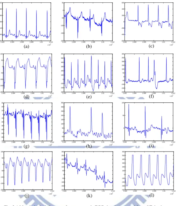
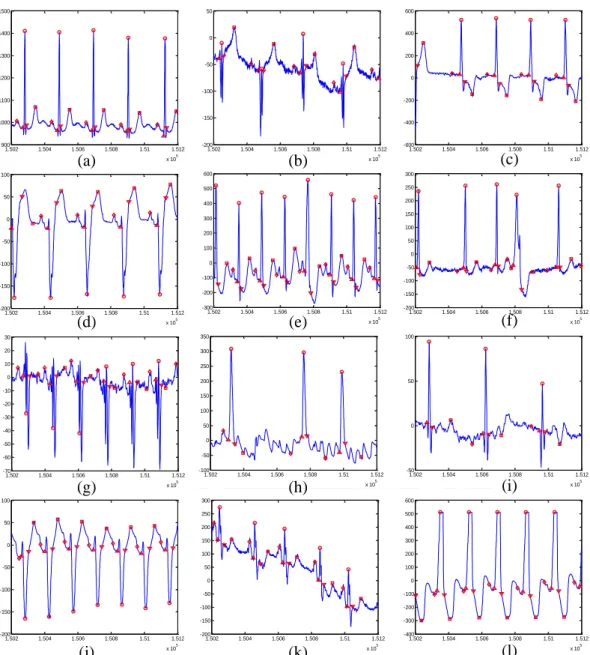
Fig. 2-1 shows some ECG signals extracted form QT database including a broad range of QRS and ST-T variety to show the morphological changes. Some non-ideal effect for mobile measurement including muscular noise, motion artifact, amplitudes changes are also shown in these examples.

11 1.502 1.504 1.506 1.508 1.51 1.512 x 105 900 1000 1100 1200 1300 1400 1500 1.502 1.504 1.506 1.508 1.51 1.512 x 105 -200 -150 -100 -50 0 50 1.502 1.504 1.506 1.508 1.51 1.512 x 105 -600 -400 -200 0 200 400 600 1.502 1.504 1.506 1.508 1.51 1.512 x 105 -200 -150 -100 -50 0 50 100 1.502 1.504 1.506 1.508 1.51 1.512 x 105 -300 -200 -100 0 100 200 300 400 500 600 1.502 1.504 1.506 1.508 1.51 1.512 x 105 -200 -150 -100 -50 0 50 100 150 200 250 300 1.502 1.504 1.506 1.508 1.51 1.512 x 105 -100 -50 0 50 100 150 200 250 300 350 1.502 1.504 1.506 1.508 1.51 1.512 x 105 -50 0 50 100 1.502 1.504 1.506 1.508 1.51 1.512 x 105 -200 -150 -100 -50 0 50 100 1.502 1.504 1.506 1.508 1.51 1.512 x 105 -200 -150 -100 -50 0 50 100 150 200 250 300 1.502 1.504 1.506 1.508 1.51 1.512 x 105 -400 -300 -200 -100 0 100 200 300 400 500 600 1.502 1.504 1.506 1.508 1.51 1.512 x 105 -70 -60 -50 -40 -30 -20 -10 0 10 20 30 (a) (b) (c) (d) (e) (f) (g) (h) (i) (j) (k) (l)

Fig. 2-1 Morphological changes of some example ECG signals extracted from QT database. Accordingly, most ECG delineation algorithm usually consists of a preprocessing stage and a decision stage. The preprocessing stage usually includes filtering of high frequency noise and baseline drift, or transforming the data into different patterns to make the features more conspicuous. Previous works of ECG QRS detection algorithm utilize methods like wavelet transform [9], band pass filtering [6], genetic algorithm [7], mathematical morphology [8], and phasor transform [10]. Among them, the multi-scale wavelet-based methods are proven to provide effective noise removal and

12

exists fast transform method which are implementation-friendly for digital implementation. Therefore, wavelet-based method is selected as the basis of the proposed delineation algorithm.

The proposed ECG delineation comprises the multi-scale dyadic wavelet transform and the feature extractor. The DWT decomposes the ECG signal and noise to different wavelet scales. And the feature extractor with search rules and adaptive threshold are applied for the ECG fiducial point decision.

2-2

Dyadic Wavelet Transform (DWT)

2-2.1

Wavelet Theory

Wavelet transform is widely used in applications such as noise reduction and edge detection and is usually implemented in the form of FIR filter banks with little hardware requirement. Wavelet transform decompose signal by a set of basis function obtained by dilation (a) and translation (b) of a single prototype wavelet ψ(t) and is defined as

𝑎𝑥(𝑏) = 1 √𝑎∫ 𝑥(𝑡) ∞ −∞ (𝑡 − 𝑏 𝑎 ) 𝑑𝑡, 𝑎 > 0. (2-1)

where Wax(b) is the wavelet coefficient at scale a, and x(t) is the original signal. The

greater the scale factor (a), the wider is the basis function. And the corresponding coefficients give information about lower frequency components of the signal.

If the prototype wavelet is defined as the derivative of a smoothing function θ(t). (2-1) can be rewritten as 𝑎𝑥(𝑏) = −𝑎 ( 𝑑 𝑑𝑏) ∫ 𝑥(𝑡) ∞ −∞ 𝜃_𝑎(t − b)𝑑𝑡. _(2-2)

13 𝜃_𝑎(t) = 1

√𝑎𝜃 ( 𝑡

𝑎). (2-3)

Then the wavelet transform at scale a can be interpreted as the derivative of the filtered version of original signal with impulse response equal to θa(t). Therefore,

every local maximum/minimum in the time domain will be represented by a zero crossing points surrounded by a positive and a negative peaks, with the amplitude of the peaks corresponded to the maximum/minimum slope. Regarding the application of detecting various ECG features occurring at different time instant coupled with different kinds of noise, the flexibility of scales and the corresponded frequency response give convenience for such application.

For discrete time signal, the dilation (a) and translation (b) can be chosen to be in dyadic form (2-4) on the time scale plane. Such kind of wavelet transform is then called dyadic wavelet transform, with basis function equal to (2-5).

a = 2𝑘_{, 𝑏 = 2}𝑘_𝑙.

(2-4)

𝑘,𝑙(𝑡) = 2− 𝑘

2 ₍₂−𝑘_{𝑡 − 𝑙). (2-5)}

According to [11], the dyadic wavelet transform can be implemented using filter banks with cascaded identical high-pass and low-pass filters as shown in Fig. 2-2 (a). To achieve the same sampling frequency and provide approximate translation invariance, algorithm á trous [12] is used. The filter response is interpolated with zero and the down sampler is removed to overcome the translation-invariance (Fig. 2-2 (b)). This is also known as the stationary wavelet transform.

14 G(z) H(z) 2 2 G(z) H(z) 2 2 G(z) H(z) 2 2 x[n] g1[n] g2[22n] g3[23n] ... G(z) H(z) x[n] G(z2) H(z2) G(z3) H(z3) g2[n] g3[n] ... (a) (b)

Fig. 2-2 (a) Mallat’s Algorithm, (b) algorithm á trous (SWT)

2-2.2

Quadratic Spline Wavelet Transform (QSWT)

A quadratic spline originally proposed in [13] is selected as the prototype waveform for the detection algorithm. The Fourier transform of this quadratic spline is depicted as

ψ( ) = ( ( )) .

(2-6)

The high-pass H(z) and the low-pass filter G(z) implemented in the DWT filter bank as in Fig. 2-2 are

H( _{) = 2 (}

2) , G( ) =

2 (

2). (2-7)

which are FIR filters with impulse response as

ℎ_𝑖[ ] =1

8× {𝛿[ + 2𝑖] + 3𝛿[ + 2𝑖−1] + 3𝛿[ ] + 𝛿[ − 2𝑖−1]}. (2-8)

15

To decide the number of scales to be used, the frequency components of some ECG signals are analyzed together with the filter bank frequency response. Fig. 2-3 shows the frequency response of the ECG signal extracted from MIT-BIH Arrhythmia Database (data 103) together with its QSWT up to 5 scales with 250Hz sampling frequency. From the figure we can see that most energy concentrate in frequency band 0 Hz to 50 Hz. Scale-1 is discarded considering the high frequency noise. Considering hardware cost and filtering performance, the proposed delineation algorithm used scale 2, 3, and 4 for detection of the 5 fiducial points (P, QRSon, R, QRSend, T).

0 200 400 600 800 1000 1200 -100 0 100 200 300 400 500 0 100 200 300 400 500 0 5000 10000 15000 N(samples@250Hz) A m p li tu d e (a) (b) Scale-2 Scale-3 Scale-4 Scale-5 0 25 50

Scale 2, 3, 4 are chosen for the proposed algorithm

Frequency(Hz)

Scale-1

75 100 125

Fig. 2-3 (a) Data #103 from MIT_BIH Arrhythmia Database at 360Hz sampling frequency and (b) the corresponded frequency response.

16

2-3

Detection Algorithm

The detection algorithm presented in this section targets for the 5 most significant ECG fiducial points (P, QRSon, R, QRSend, and T) based on the quadratic spline wavelet transform described in the previous section. The dyadic wavelet transform filter out the interference of high frequency noise and baseline drift and decompose the ECG signal into different scales. Detection is then performed based on the cross examination among these scales of coefficients. Comparing with existing off-line detection methods with costly computation, the proposed algorithm is designed suitable for hardware implementation providing comparable detection result. The detection rules for each feature and the adaptive generation for threshold and search window will be described in the following paragraphs.

2-3.1

Wave Characteristic and Detection Flow

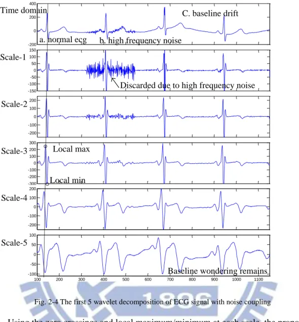
Fig. 2-4 shows the decomposition of some example ECG waveform using the QSWT. From the figure we can see that a peak in the time domain will be represented by a zero crossing point surrounded by a local maximum and minimum point in the wavelet domain, each representing the deepest rising and falling slope. The reason for discarding scale-1 becomes clear in this figure (high frequency noise). For the 5 desired fiducial points with different wave characteristics, detections are done using different scales of wavelet coefficients. For the most important R peak, we use scale 2, 3, 4 for detection. Because of reduced resolution in higher scales, sharp edges such as the boundary for QRS complex (i.e. QRSon, QRSend) use coefficients of scale-2 for detection. Wide wave such as P and T wave use higher scales (scale-4) for detection. Considering hardware cost, increased latency in higher scales, and the interference of baseline drift, the scale of wavelet decomposition is limited to four.

17 100 200 300 400 500 600 700 800 900 1000 1100 -200 0 200 400 100 200 300 400 500 600 700 800 900 1000 1100 -150 -100 -50 0 50 100 150 100 200 300 400 500 600 700 800 900 1000 1100 -200 -100 0 100 200 100 200 300 400 500 600 700 800 900 1000 1100 -300 -200 -100 0 100 200 300 100 200 300 400 500 600 700 800 900 1000 1100 -200 -100 0 100 200 100 200 300 400 500 600 700 800 900 1000 1100 -100 -50 0 50 100 Time domain Scale-1 Scale-2 Scale-3 Scale-4 Scale-5

Discarded due to high frequency noise a. normal ecg b. high frequency noise

C. baseline drift

Baseline wondering remains Local max

Local min

Fig. 2-4 The first 5 wavelet decomposition of ECG signal with noise coupling

Using the zero crossings and local maximum/minimum at each scale, the proposed algorithm detects the five fiducial points within a cardiac cycle by:

a) Detection for R peak.

b) Search-back for QRSon and P wave. c) Moves on for QRSend and T wave.

18 Wavelet Transform Threshold update Cardiac Cycle R Peak Detection QRSon Decision T Peak Detection scale 4 scales 2,3,4 scale 4 ECG P Peak Detection QRSoff Detection Scale 2, 4 P/T Search Window update Search back Search forward scales 2,3,4 scale 2 If an R peak is detected

· The detection threshold for R peak detection and boundary detection is updated every time an R peak is detection

· Search for P and T detection is limited in the P/T search window

· End of delineation of an cardiac cycle

· Delineation is performed based on a 4-scale wavelet transform

· Once an R peak is detected, delineation for other fiducial points starts

Fig. 2-5 Flow graph for the proposed detection algorithm

Fig. 2-5 shows the flow graph of the detection algorithm. For the best extraction performance, the feature extraction process starts with the most obvious R peak. Based on the detected R peak, the detector searches back for the starting boundary of the QRS complex (i.e. QRSon) and P wave. After successful search of these wave points, the detection moves forward for QRSend and T wave. This completes the detection of the 5 wave within a cardiac cycle. To reduce unnecessary search time and power, the detection for P and T wave is limited in a search window. The search window and the detection thresholds for locating the peaks are updated every cardiac cycle.

19

Considering hardware cost, the design rules for QRSon/end and P/T waves are designed to be similar so the hardware can be shared. The detection detail will be explained as follows.

2-3.2

R Peak Detection

Scale-2

Zero crossing

Local max

Thresholds are updated every time an R peak is

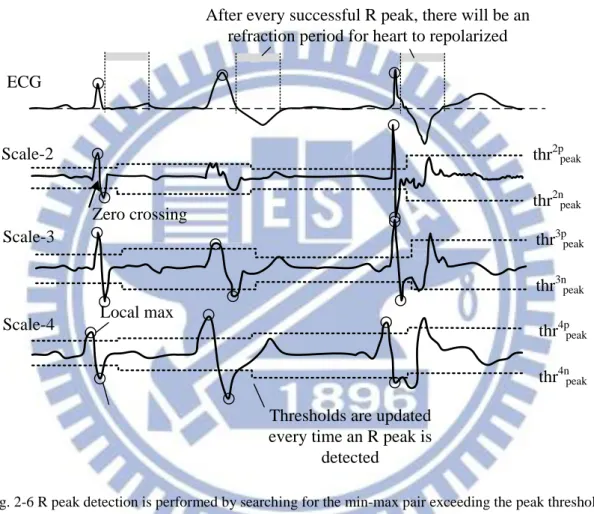
detected thr2p Scale-4 ECG peak thr2npeak thr3ppeak thr3npeak thr4ppeak thr4npeak Scale-3

After every successful R peak, there will be an refraction period for heart to repolarized

Fig. 2-6 R peak detection is performed by searching for the min-max pair exceeding the peak threshold in scale 2, 3, and 4

A peak is indicated by the temporal relationship of local minimum and maximum peak pair defined as the point exceeding the peak threshold (

thr

_peak2p ,

thr

_peak2n , etc.) together with the zero crossing between them. The detection of R peak is performed with cross examination in the 3 scales (scale-2, 3, and 4) because of its high importance. To prevent large data storage, the detection is done sequentially using 3 parallel state machines. According to the 3 scales of wavelet coefficients, the state

20

machines change state when finding a positive or negative peak, a zero crossing point, and the proceeding peaks opposite to the previous detected peak, and output the marking for possible candidate for QRS complex. Using the rule of majority, if candidate markings are found in 2 or more scales, the zero crossing point in scale-2 will be considered as the detected R peak. Besides locating the R peak location, the information of this min-max pair (amplitude, location) is recorded for successive QRSend detection and threshold update.

After successful locating an R peak, the conducting cell needs to repolarize in order contract again. This period is called the refraction period. During this period, no peak will be considered as R peak.

2-3.3

QRS

on/end

Detection

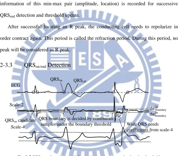
QRSon Scale-2 thr2p Scale-4 ECG boundary thr2n QRS boundary is decided by continuous

samples under the boundary threshold

QRSoff

Wide QRS needs coefficients from scale-4

QRSon candidate

boundary

Fig. 2-7 QRSon/end detection search for continuous samples under the edge threshold

Considering reduced resolution in higher scales, coefficients of scale-2 is used of detection of QRS edges (QRSon/end). Because of similar wave characteristic, the detection rules for QRSon/end detection are designed to be the same so the hardware can be shared (with only comparators). The detection of QRSon/end is performed by searching for continuous points under the boundary threshold as illustrated in Fig. 2-7.

21

The detection of QRSend can be performed following successful detection of R peak. To avoid search back and additional storage for QRSon detection, possible points satisfying the detection rules are saved as QRSon candidates. Finally the candidate that supplies the most nearest sample to the R peak will be confirmed as the real QRSon point.

To avoid morphological changes of wide QRS complex (syndrome: PVC-premature ventricular contraction) which cannot be characterized by scale-2, coefficients of scale-4 is used to distinguish the wide morphology and avoid detecting false boundary (shown in the right part of Fig. 2-7).

2-3.4

P/T Wave Detection

P Scale-4 ECG _{T P} T P T P search window T search window QRSon-end

Search window is calculated from

recursive computation of QRSon-end interval zero crossing

Fig. 2-8 Search window defined for P/T detection

Because of the wider wave characteristic, the detection process of P and T wave detection use scale-4 for detection. The process is as follows: First, the search is limited in a search window defined relatively according to the recursive computing of QRSon to QRSend interval. This reduces extra time and power for unnecessary search according to the physical phenomenon for a normal cardiac cycle. Instead of using RR interval as reference, QRSon to QRSend interval eliminates the influence of

22

morphological changes of QRS complex. The size of the search window is carefully designed because it results in extra storage for P wave search back after R peak detection. Finally we define the search window boundary for P and T wave detection to be: 𝑆𝑊𝑝𝑟 = 10. 𝑆𝑊_𝑝𝑙= {_{10 + 𝑄𝑅𝑆} 100 𝑓(𝑆𝑊𝑝𝑙 > 100) 𝑜𝑛−𝑒𝑛𝑑× 0.375. . 𝑤. . ( 2-10 ) 𝑆𝑊_𝑡𝑙 = 15. 𝑆𝑊_𝑡𝑟 = {_{15 + 𝑄𝑅𝑆}100 𝑓(𝑆𝑊𝑡𝑟 > 100) 𝑜𝑛−𝑒𝑛𝑑× 0. . . 𝑤. . ( 2-11 )

with a maximum search range of 100 samples under 250Hz sampling frequency. The QRSon-end is the value that updated every time a new QRS complex is detected. These values are designed according to the physical nature of our heart. For example, the value of SWpr is chosen to be 10 because the delay caused by AV node between atrial and ventricular is approximately 0.1 second.

Within this window, we search for the global maximum/minimum points. If one of them exceeds the P/T threshold, a wave is considered to exist and is indicated by the zero crossing point between them.

2-3.5

Adaptive Threshold and Window Update

As mentioned previously, the robustness of the proposed algorithm lies from the adaptively update of detection parameters including the peak threshold for R peak detection and the boundary threshold for QRSon/end detection and the search window for P and T wave detection.

23

For R peak detection, separate thresholds (

thr

_peakxp ,

thr

_peakxn ) are used for positive and negative peaks to avoid failed detection for asymmetric rise and fall peaks shown in Fig. 2-6. Avoiding costly computation such as division, square roots [14], or root-mean-square [9], thresholds are computed based on the information of the recorded value of local min-max pair (signal peak) and the recorded noise level (noise peak). The equation of the peak threshold for R peak detection and boundary threshold for QRSon/end detection are depicted as follows:

{ 𝑓 (𝑙 𝑎𝑙_𝑚𝑎𝑥𝑥 ≥ 𝑡ℎ𝑟𝑝𝑒𝑎𝑘 𝑥𝑝 _{) → 𝑆𝑃} 𝑝𝑒𝑎𝑘𝑥𝑝 . 𝑒𝑙 𝑒 𝑓 (𝑙 𝑎𝑙_𝑚𝑎𝑥_𝑥 < 𝑡ℎ𝑟_{𝑝𝑒𝑎𝑘}𝑥𝑝 ) → 𝑁𝑃_{𝑝𝑒𝑎𝑘}𝑥𝑝 . (positive threshold) { 𝑓 (𝑙 𝑎𝑙_𝑚 𝑥 ≥ 𝑡ℎ𝑟𝑝𝑒𝑎𝑘 𝑥𝑛 _{) → 𝑆𝑃} 𝑝𝑒𝑎𝑘𝑥𝑛 . 𝑒𝑙 𝑒 𝑓 (𝑙 𝑎𝑙_𝑚 𝑥< 𝑡ℎ𝑟𝑝𝑒𝑎𝑘𝑥𝑛 ) → 𝑁𝑃𝑝𝑒𝑎𝑘𝑥𝑛 . (negative threshold)

where x is the scale.

(2-12) 𝑡ℎ𝑟_{𝑝𝑒𝑎𝑘}𝑥𝑝 ′ = 𝑡ℎ𝑟_{𝑝𝑒𝑎𝑘}𝑥𝑝 × 3 + 𝑁𝑃_{𝑝𝑒𝑎𝑘}𝑥𝑝 + (𝑆𝑃_{𝑝𝑒𝑎𝑘}𝑥𝑝 − 𝑁𝑃_{𝑝𝑒𝑎𝑘}𝑥𝑝 ) ≫ 1 𝑡ℎ𝑟_{𝑝𝑒𝑎𝑘}𝑥𝑛 _{′ = 𝑡ℎ𝑟} 𝑝𝑒𝑎𝑘𝑥𝑛 × 3 + 𝑁𝑃𝑝𝑒𝑎𝑘𝑥𝑛 + (𝑆𝑃𝑝𝑒𝑎𝑘𝑥𝑛 − 𝑁𝑃𝑝𝑒𝑎𝑘𝑥𝑛 ) ≫ 1 (2-13) 𝑡ℎ𝑟_{𝑏𝑑𝑟𝑦}𝑝 = 𝑡ℎ𝑟_{𝑝𝑒𝑎𝑘}2𝑝 ≫ 𝑡ℎ𝑟_{𝑏𝑑𝑟𝑦}𝑛 _{= 𝑡ℎ𝑟} 𝑝𝑒𝑎𝑘2𝑛 ≫ (2-14)

Equation (2-12) describes the rule to classify the noise peak and signal peak. The new threshold is computed by the weighted average of the current threshold and the new threshold based on the detected noise peak and signal peak (2-13). Equation (2-14) shows that the threshold for QRS complex boundary detection is based on a simple shift of the peak threshold.

24

2-4

Simulation Result and Performance Evaluation

Fig. 2-9 shows the detection result of the proposed algorithm with different wave morphologies and noise coupling.

1.502 1.504 1.506 1.508 1.51 1.512 x 105 900 1000 1100 1200 1300 1400 1500 1.502 1.504 1.506 1.508 1.51 1.512 x 105 -200 -150 -100 -50 0 50 1.502 1.504 1.506 1.508 1.51 1.512 x 105 -600 -400 -200 0 200 400 600 1.502 1.504 1.506 1.508 1.51 1.512 x 105 -200 -150 -100 -50 0 50 100 1.502 1.504 1.506 1.508 1.51 1.512 x 105 -300 -200 -100 0 100 200 300 400 500 600 1.502 1.504 1.506 1.508 1.51 1.512 x 105 -200 -150 -100 -50 0 50 100 150 200 250 300 1.502 1.504 1.506 1.508 1.51 1.512 x 105 -100 -50 0 50 100 150 200 250 300 350 1.502 1.504 1.506 1.508 1.51 1.512 x 105 -50 0 50 100 1.502 1.504 1.506 1.508 1.51 1.512 x 105 -200 -150 -100 -50 0 50 100 1.502 1.504 1.506 1.508 1.51 1.512 x 105 -200 -150 -100 -50 0 50 100 150 200 250 300 1.502 1.504 1.506 1.508 1.51 1.512 x 105 -400 -300 -200 -100 0 100 200 300 400 500 600 1.502 1.504 1.506 1.508 1.51 1.512 x 105 -70 -60 -50 -40 -30 -20 -10 0 10 20 30 (a) (b) (c) (d) (e) (f) (g) (h) (i) (j) (k) (l)

Fig. 2-9 Detection result of the proposed with ECGs with morphological changes and noise As there is no golden rule for the decision for peaks, onset, and endset, the validation for the detection result needs to be performed by doctors. Thanks to Physionet [3], lots of standard databases are provided and sorted with detail information about the ECG including the corresponded syndrome and either manually

25

or automatically annotated fiducial points. In this report, we choose the two common databases for the validation of our proposed algorithm, namely the MIT-BIH Arrhythmia Database (MITDB) [4] and QT Database (QTDB) [5]. Here we first make a brief introduction about the databases and provide the validation result.

 MIT-BIH Arrhythmia Database (MITDB) [4]

The MITDB includes 48 specially selected Holter recordings with anomalous but clinically important phenomena at 360Hz sampling frequency, 11-bits resolution and 10-mV amplitude range with automatically determined R peak annotations. We use this database for the validation for R peak detection.

 QT Database (QTDB) [5]

The original goal for QTDB is to make a database with sufficient ECGs coverage for variety of QRS and ST-T morphologies in order to challenge existing algorithms with real-world variability. The 105 records were chosen primarily from among existing ECG databases, including the MITDB, the European Society of Cardiology ST-T Database [4], and several other ECG databases collected at Boston's Beth Israel Deaconess Medical Center. All records all resample to 250Hz in QTDB. Different annotations are provided including the automatically annotation for QRS complex (.man) and manually determined waveform boundaries by two experts (.q1c .q2c). We validate the detection result of all the fiducial points using this database.

The two parameters to qualify the detection result are sensitivity (Se) and positive predictivity (Pr) and are depicted as

𝑆𝑒 = 𝑇𝑃

𝑇𝑃 + 𝐹𝑁, Pr = 𝑇𝑃

𝑇𝑃 + 𝐹𝑃. (2-15)

where TP stands for true positive detection, FN stands for false negative detection, and FP stands for false positive detection. The sensitivity Se reports the percentage of true

26

beats that were correctly detected. The positive predictivity Pr reports the percentage of beat detections which were in real true beats (accuracy).

Comparison of the detection result with the state-of-the art detection algorithm (including software algorithm and hardware detector) are also listed in Table 2-1 and Table 2-2. Table 2-3 lists the detail detection result of R peak detection verified using MITDB.

Table 2-1 R peak detection comparison with state-of-the-art detector using MITDB

Detector # Annotation TP FP FN Se (%) Pr (%) This work Wavelet Transform hardware 109980 109632 317 348 99.71 99.68 [9] 2004 TBE

Wavelet Transform software 109428 109208 153 220 99.80 99.86 [10] 2010 PMea

Phasor Transform software 109428 109111 35 317 99.71 99.97 [17] 2012 TBCAS

Wavelet Transform hardware 109134 108381 330 753 99.31 99.70 [16] 2010 ISCAS

Filtering, Diff, Square hardware N/A N/A N/A N/A 95.65 99.36 [15] 2009 TBCAS

Mathematical Morphology

hardware N/A 109510 213 214 99.81 99.80 [14] 2009 ASSCC

Wavelet Transform hardware 109492 108892 117 500 99.63 99.89 Table 2-2 Fiducial points delineation result comparison using QTDB

Detector P QRSon QRSend T

Se (%) Pr (%) Se (%) Pr (%) Se (%) Pr (%) Se (%) Pr (%)

This work

Wavelet Transform 99.59 96.11 99.97 100.00 99.97 100.00 99.38 99.41

[9] 2004 TBE

Wavelet Transform 98.87 91.03 99.97 N/A 99.97 N/A 99.77 97.79 [10] 2010 PMea

27

Table 2-3 R peak detection result within MITDB

Records Total (beats) TP FP FN Se (%) Pr (%)

100 2272 2272 1 0 100.00 99.96 101 1864 1863 2 1 99.95 99.89 102 2186 2186 1 0 100.00 99.95 103 2084 2082 0 2 99.90 100.00 104 2228 2225 32 3 99.87 98.58 105 2585 2562 64 23 99.11 97.56 106 2018 2009 5 9 99.55 99.75 107 2135 2131 1 4 99.81 99.95 108 1809 1796 8 13 99.28 99.56 109 2530 2524 3 6 99.76 99.88 111 2123 2123 17 0 100.00 99.21 112 2537 2537 5 0 100.00 99.80 113 1794 1794 0 0 100.00 100.00 114 1878 1878 10 0 100.00 99.47 115 1953 1953 0 0 100.00 100.00 116 2396 2388 1 8 99.67 99.96 117 1534 1534 4 0 100.00 99.74 118 2277 2277 2 0 100.00 99.91 119 1986 1986 1 0 100.00 99.95 121 1862 1860 1 2 99.89 99.95 122 2475 2474 2 1 99.96 99.92 123 1518 1518 1 0 100.00 99.93 124 1619 1618 1 1 99.94 99.94 200 2598 2595 7 3 99.88 99.73 201 1962 1949 3 13 99.34 99.85 202 2136 2130 0 6 99.72 100.00 203 2986 2936 25 50 98.33 99.16 205 2655 2651 1 4 99.85 99.96 207 2323 2238 25 85 96.34 98.90 208 2954 2939 3 15 99.49 99.90 209 3005 3004 5 1 99.97 99.83 210 2651 2626 4 25 99.06 99.85 212 2747 2747 2 0 100.00 99.93 213 3251 3242 1 9 99.72 99.97 214 2261 2255 3 6 99.73 99.87 215 3364 3363 1 1 99.97 99.97 217 2207 2203 2 4 99.82 99.91 219 2157 2153 1 4 99.81 99.96 220 2047 2047 0 0 100.00 100.00 221 2426 2419 2 7 99.71 99.92 222 2484 2479 5 5 99.80 99.80 223 2604 2596 1 8 99.69 99.96 228 2057 2039 35 18 99.12 98.31 230 2257 2256 1 1 99.96 99.96 231 1571 1571 0 0 100.00 100.00 232 1783 1780 25 3 99.83 98.61 233 3078 3072 1 6 99.81 99.97 234 2753 2752 2 1 99.96 99.93 Total 109980 109632 317 348 99.71 99.68

28

From Table 2-1, the proposed algorithm achieves 99.71% sensitivity and 99.68% positive predictivity for R peak detection. Although with reduced computation complexity, the performance of the proposed algorithm is still compatible with the published off-line detection algorithms. Our algorithm achieves similar detection accuracy comparing with the on-line detection ASICs.

Table 2-2 shows the detection result of other targeted fiducial points (P, QRSon, QRSend, T) comparing with the 2 off-line detector verified using QTDB q1c annotation. The proposed algorithm achieves better detection result at QRSon and QRSend detection and similar result for P and T wave detection.

2-5

Summary

In this chapter we proposed an ECG delineation algorithm especially for abnormal alarm based on 4-scale quadratic spline wavelet transform. The delineation algorithm can extract P, QRSon, R, QRSend, and T wave with accuracy over 99%. The wavelet transform removes noise interference and decompose ECG signal into different frequency bands. With cross examination among the decomposed scales and adaptive threshold update considering noise level, the algorithm is suitable for mobile ECG monitoring. Designed using only simple operations, the algorithm can be implemented using low power ASICs. Chapter 4 describes the architecture for the implemented ASIC delineator, using mixed synchronous and asynchronous design style with low power techniques.

29

Chapter 3:

Asynchronous Design

In this chapter, we first provide the motivation for going from synchronous design to asynchronous design, the advantages and disadvantages. Then we introduce the basic theory for asynchronous design. A 2-phase handshake protocol modified from the MOUSETRAP [21] pipeline for iterative computation is proposed and tested. Design flow using commercial CAD tool is also provided, making asynchronous design an option for synchronous designers with standard cells. In the end, an example design of an energy-efficient 16-tap FIR filter is built to make comparison between asynchronous and synchronous design.

3-1

Motivation

0.5 1 1.5 0 50 100 150 200 250 0.5 1 1.5 0 50 100 150 200 250

Normalized delay (delay/μ) 1V, 25°C σ/μ=0.0376 0.5V, 25°C σ/μ=0.0990 O cc u re n ce s

Fig. 3-1 The Monte Carlo simulation with intra-die variation of 3 sigma using UMC 90nm process under 1.0V and 0.5V supply voltage respectively

Voltage scaling is a common technique to reduce the power consumption in circuit design. However, as the supply voltage is scaling down, circuit propagation delay becomes extremely sensitive to PVT variation. Hence, large delay margin is required

30

for successful operation for synchronous design. However, for asynchronous circuit, the operation speed is decided by the handshakes between registers instead of the global worst case clock cycle. This average case design can therefore result in faster operation speed or lower power consumption.

Fig. 3-1 shows the Monte Carlo simulation for the delay of the critical path in a multiplied accumulator (MAC) under 1.0V and 0.5V supply voltage. The figure clearly shows that the delay variance at 0.5V is approximately three times larger than the variance at 1.0V because synchronous design uses the worst case as its operation condition. Large safety timing margin is wasted for synchronous design.

Besides combating PVT variation under low supply voltage, asynchronous circuit is also an attractive technique for low-speed systems with event-driven asynchronous functions that are activated only when certain event occurred. Asynchronous design provides power management with low latency and removes the requirement for additional high speed clock. Simple handshake interface also makes it easy for system integrations between asynchronous and synchronous potion.

3-2

Introduction to Asynchronous Circuit

3-2.1

Moving from Synchronous to Asynchronous Approach

Synchronous designs use a global clock to synchronize the whole design. Besides dealing with severe PVT variations under low supply voltage, uncertainty of clock source is another important issue. Clock skew and jitter together with the logic propagation variation under low supply voltage makes synchronous approach an inefficient design for low supply systems. Although current CAD tools provide powerful algorithm to generate clock trees, the well-spread buffers and delay cells still results in large power overhead.

31

Unlike synchronous design, asynchronous design replaces the synchronous global clock into locally handshake circuit. Fig. 3-2 shows a common pipeline structure for both synchronous design and asynchronous design. The red part shows the replacement from global clock to locally handshake circuit. There are numerous approaches to designing without clocks, each with various pros and cons depending on the design style. Some of the major potential benefits include the follows.

 Robust operation against PVT variation due to elimination of fixed clock.  Modular composition and delay insensitive interfacing.

 Power management with very low latency.

However, some significant potential drawbacks still exits for clock-less designs includes:

 Complicated design approaches unfamiliar for synchronous designer  Lack of support from existing EDA tools

 Area and performance overhead for handshake circuits

Therefore, one must be clear about the properties of asynchronous designs when applying it to the system, giving its advantages and reduce the overhead as much as possible to deliver an efficient design. The next part will be some introduction to the basic asynchronous pipeline style and handshake protocol.

R1 R2 LOGIC R3 CLK R1 R2 LOGIC R3 HS1 HS2 HS3 DELAY R1 R2 LOGIC R3 HS1 HS2 HS3 REQ ACK ACK (a) Synchronous

(b) Asynchronous Pipeline - Bundled Delay

(c) Asynchronous Pipeline – Dual Rail REQ ACK

ACK Clock tree

32

3-2.2

Handshake Protocol

The two most common asynchronous design styles are the bundled-delay asynchronous pipeline (Fig. 3-2 (b)) and dual rail asynchronous pipeline (Fig. 3-2 (c)). A brief introduction is made here above the two asynchronous

 Dual rail asynchronous pipeline

One common type of the quasi delay insensitive circuits is the dual rail asynchronous design. Dual rail design encodes the arrival information into the data bit itself. Therefore, two bits are required to represent the arrival of one-bit information which makes the design “dual rail”. Table 3-1 shows a dual rail encoding scheme. With this kind of encoding, two parties can communicate reliably regardless of the delay variations. However, additional dual rail datapath and storage results in large area and power penalties. Although customized gates can be designed to reduce the overhead, the design process is too much effort and time costly for synchronous designer.

Table 3-1 One encoding scheme for dual rail encoding State True rail False rail

Null 0 0

Logic 0 0 1

Logic 1 1 0

N/A 1 1

 Bundled-delay asynchronous pipeline

The bundled-data asynchronous designs are conceptually closest to synchronous design. Each datapath through a combination block is matched with a delay line with the same propagation delay. Because of this “bundled” delay line, this type of asynchronous circuit is called “bundled delay” or “matched delay”. Thanks to the similarity with synchronous design, we can use standard cells and commercial CAD tool with costumized design constraints to implement the design.

33

Handshake circuit can also be categorized using the number of phase that is required for one data transmission. The most common protocols are the 4-phase and 2-phase handshake protocol. The 4-phase handshake protocol, also named “Return-to-Zero (RTZ)” or level triggered protocol, uses logic “1” to signal data valid, therefore simple transparent latches can be used as pipeline registers. However, additional return-to-zero operation is required for the start of the next handshake, which results in additional switching and time. To reduce the extra RTZ time, AND delay line configured as Fig. 3-3 (c) [19] can be used to force the output to zero once the input goes to zero.

The 2-phase handshake protocols, also named non return-to-zero (NRTZ) or transition signaling protocol, use signal transitions as signal event, no addition RTZ is required, but more complex handshake circuit or latched may be needed for recognition of both positive and negative edges.

Ack Req

Ack Req

DATA

(a) 4-phase protocol (b) 2-phase protocol

DATA

IN . . . OUT

(c) AND delay line

34

3-2.3

Muller C Element

One of the basic components that are generally used in asynchronous design is the Muller C-element cell [20]. The output reflects the input when all the input matches. Fig. 3-4(a) shows the symbol and truth table of a 2-input C element. Such kind of function can be implemented using either by standard NAND gates (Fig. 3-4(a)) or by customized transistors level construction (Fig. 3-4 (b)).

C element is the basic gate for the famous Muller pipeline [20]. Because of its unique function, it can also be used in fork and join structures (Fig. 3-5). Fork structure is used when one request is sent to more than two recipients. The corresponded acknowledge signal will consist of a join structure using C element (Fig. 3-5(a)) and vice versa for conditions when two requests are being combined to one recipient (Fig. 3-5(b)). C A B Z A B OUT B A B A OUT VDD VSS (b) (c) Z B A 0 0 0 Zn-1 1 0 0 1 1 1 1 Zn-1 (a)

Fig. 3-4 (a) Symbol and truth table of a 2 input C element (b) Standard cell based C element (c) Transistor level implementation

35 C C Req Fork Join Fork Join Ack Req0 Req1 Ack0 Ack1 Req0 Req1 Ack0 Ack1 Req Ack (a) (b)

Fig. 3-5 Fork and join structures

3-2.4

Asynchronous Pipelines

Here a brief introduction about 2 existing asynchronous pipelines is presented: The 4-phase Muller pipeline [20] and 2-phase minimal-overhead ultra-high-speed transition-signaling asynchronous pipeline (MOUSETRAP) [21], including the structure and working mechanism. Both of the pipelines are bundled-delay pipelines.  4-phase Muller pipeline [20]

L1 L2 LOGIC L3 DELAY C C C ACK REQ ACK REQ DATA DATA

Fig. 3-6 Muller pipeline

Muller pipeline is the backbone for many other variations and extensions of asynchronous pipeline. Simple handshake circuit is built using only inverters and C element. To understand the handshake working mechanism, we first assume all the

36

outputs of C element are reset to zero. A firing of 0 to1 from the left REQ will make the output of the first C element to 1 and triggered the first latch R1. This request signal will propagate through the pipeline stages together with the data. When the successor receives the request, an acknowledge signal will be sent back to the predecessor, and the predecessor will be able to receive the new data. With no costumed cell and simple timing constraint, this pipeline style is suitable to build using commercial CAD tools.

 2-phase MOUSETRAP pipeline [21]

L1 L2 LOGIC L3 DELAY ACK REQ ACK REQ DATA DATA

Fig. 3-7 MOUSETRAP pipeline

The MOSETRAP pipeline is a 2-phase pipeline style that can be constructed using simple transparent latch while other 2-phase pipeline style may require special designed latched to capture the transition of 2-phase protocols. The handshake circuit consists of a latch and a XNOR gate. With all handshake latches reset to zero, each latch is transparent before the data arrives. Upon receiving the arrival of a transition on the request signal, the latch captures the data and becomes opaque. The REQ transition and the data propagate continuously to the next stage, and are again captured. An acknowledge signal is sent back to the predecessor, enabling the predecessor and makes it transparent again in order to capture new data.

37

3-3

Design Flow Using Commercial CAD Tool

While asynchronous designs can prove substantial benefits, it is still largely limited by the incompatibility with existing CAD tool. Here we attempt a design flow based on relative timing and post-layout SPICE verification, to create and prove correct constraints for the bundled-delay asynchronous pipeline using the mature timing engine from existing CAD tool. These constraints are supported by most CAD tools and support timing driven synthesis and auto place and route.

3-3.1

Design flow

The signal in bundled-delay designs can be separated into two parts, the signal part and the control part. In this flow, we use the following CAD tools together with some .sdc constraint to complete the design for the 4-phase Muller pipeline and 2-phase MOUSETRAP pipeline. Table 3-2 shows the CAD tool and the constraints used in this asynchronous design flow.

Table 3-2 CAD tools and design constraints used in the asynchronous design flow

CAD Tool Design Constraints

Tech: UMC 90nm RTL: Verilog

Synthesis: Synopsys Design Compiler P&R: Cadence SOC Encounter Verification: Ultrasim (SPICE Model)

set_dont_touch set_size_only set_max_delay set_min_delay set_disable_timing

To start, we first construct a template model using standard cells at gate level for the handshake circuit (control part). For the Muller pipeline, it would be like the one shown in Fig. 3-8.

38

Structure modification may occur during synthesis when optimization, such as removing buffer or back-to-back inverters, breaking complex gate into simple gates, which may result in hazard or substantially modify necessary delay properties. Constraints “set_dont_touch” and “set_size_only” are used to prevent this from happening. The “set_dont_touch” command disallow the tools to change the cells in any kinds of ways while “set_size_only” command prevents change of cells but still allow the tool to change cell size of driving strength, delay, and power optimization.

C L_ACK L_REQ R_ACK R_REQ EN

Fig. 3-8 A Verilog template for the Muller pipeline template

set_size_only -all_instance {*/c_ele0_nand0} set_size_only -all_instance {*/c_ele0_nand1} set_size_only -all_instance {*/c_ele0_nand2} set_size_only -all_instance {*/c_ele0_nand3} set_size_only -all_instance {*/hs0_inv}

39

Clock CAD tools use clock domain to optimize power and performance based on the defined frequency. These tools operate based on directed acyclic graph (DAG). If the timing got loops, algorithms in the tool are called to break it. In asynchronous design there are plenty of feedback loops either in the standard cell based C element or in the protocol cycles. Cutting theses loops at the right place is necessary for correct and efficient timing analysis and optimization. The command “set_disable_timing” does the job. For example, we can use this command to break the acknowledge path that has no timing requirement but ends up in timing loops.

C C

L_ACK

L_REQ

Timing loops Cut the timing loops at the ack path

R_ACK

R_REQ

HS0 HS1

Fig. 3-9 Break timing loops for un-constraint path

set_disable_timing -from HS1/L_ACK -to HS0/R_ACK

Beside the control part, the registers and datapath can be generated using the standard flow used in synchronous design expect that in synchronous design, the maximum delay is decided by the required clock cycle. In bundled-delay asynchronous design, there’s no clock defined. The maximum delay for the datapath and matched delay is set manually by the “set_max_delay” and “set_min_delay”.

40 L2 LOGIC L3 DELAY C C DATA L_ACK L_REQ

Set max delay: 10.0ns Set min delay:11.0ns

R_ACK

R_REQ

Fig. 3-10 Time constraints should be set manually at the desired start and end points

set_max_delay 10.0 -from L2_reg[*] -to L3_reg[*]

set_min_delay 10.5 -rise_from DELAY/IN -rise_to DELAY/OUT set_max_delay 11.0-rise_from DELAY/IN -rise_to DELAY/OUT

In this example the maximum delay from register L2 to register L3 is set to 10.0ns and the minimum delay is set to 10.5ns with a 5% safety margin. The next section will discuss the additional margin in detail based on Monte-Carlo simulation using UMC 90nm technology. After applying the above .sdc constraint, the design is ready for synthesis. The function is verified at gate-level. The same constraints can be applied again for backend place and route.

3-3.2

Delay Margin Tuning

Bundled-delay asynchronous relies on correct handshake and relative timing between delay line and datapath to compute the correct function. In the previous section, we mentioned that additional margin is required between the matched delay and datapath. Large margins results in wasted computation time but small margin may generate false output which cannot be solved. Here some Monte-Carlo simulation is

41

made to estimate the margin range and a lead-lag detector is proposed for margin tuning.

In the example, we extract the critical path in an 8×8+16bit multiplied accumulator (MAC) and produced a matched delay line using worst-case standard cell library. 5000 times Monte Carlo simulation is done with intra-die variance of 3 sigma at 3 different corner case ({0.45V, -40°C}, {0.5V, 25°C}, {0.55V, 120°C}). In the simulation, we assume the global voltage and temperature are the same because of the small design size. Fig. 3-11 shows the simulation result.

0 2 4 6 8 10 12 14 16 18 20 0 100 200 300 400 500 600 700 800 900 1000 datapath@0.5V, 25C delay@0.5V, 25C 0 2 4 6 8 10 12 14 16 18 20 0 50 100 150 200 250 300 350 400 datapath@0.45V, -30C delay@0.45V, -30C 0 2 4 6 8 10 12 14 16 18 20 0 200 400 600 800 1000 1200 1400 1600 1800 datapath@0.55V, 120C delay@0.55V, 120C -1 0 1 2 3 4 5 0 100 200 300 400 500 600 700 800 delay-datapath diff @ 0.5V, 25C delay-datapath diff @ 0.45V, -30C delay-datapath diff @ 0.55V, 120C (a) 0.5V, 25°C _{(b) 0.45V, -30°C}

(c) 0.55V, 120°C (d) Difference between datapath and delayline at 3 different corners

delay(ns) Occurance delay(ns) Occurance delay(ns) delay(ns) Occurance Occurance

Fig. 3-11 The delay distribution of datapath and delay line at 3 different corner case (a) 0.5V, 25°C (b) 0.45V, -30°C (c) 0.55V, 120°C (d) Difference between datapath and delay line