砷化鎵/砷化鋁異質結構之Γ -Χ 反交叉能隙理論分析

全文

(1)國立交通大學電子工程學系電子研究所碩士班碩士論文. 砷化鎵/砷化鋁異質結構之 Γ − Χ 反交叉能隙理論分析. Theoretical investigation of Γ - Χ anticrossing gaps of GaAs/AlAs heterostructures. 研究生：簡立欣指導教授：顏順通博士. 中華民國九十四年七月.

(2) 砷化鎵/砷化鋁異質結構之 Γ − Χ 反交叉能隙理論分析 Theoretical investigation of Γ - Χ anticrossing gaps of GaAs/AlAs heterostructures. 研究生：簡立欣. Student：Chien Li-Hsin. 指導教授：顏順通博士. Advisor：Dr. Shun-Tung Yen. 國立交通大學電子工程學系電子研究所碩士論文. A Thesis Submitted to Department of Electronics Engineering & Institute of Electronics College of Electrical Engineering and Computer Science National Chiao Tung University in partial Fulfillment of the Requirements for the Degree of Master in Electrical Engineering June 1997 Hsinchu, Taiwan, Republic of China. 中華民國九十四年七月.

(3) 砷化鎵/砷化鋁異質結構之 Γ − Χ 反交叉能隙理論分析. 學生：簡立欣. 指導教授:顏順通教授. 國立交通大學電子工程學系電子研究所碩士班摘要. 本篇論文提出一個新穎的想法來產生微分負阻的機制，並且可用來實現兆赫波震盪器。這個震盪器利用砷化鎵/鋁化鎵異質結構本身的特性—電子可以從 Γ 點遷移到 X 點而不用有聲子的參與。和傳統的 Gunn 震盪器比較，此震盪器的震盪頻率不受限於電子—聲子的散射機率。因此，微分負阻的機制主要是由 Γ–X 耦合的機制來控制，此時反交叉能隙是決定 Γ–X 耦合強度的一個重要參數。在本篇研究中所採用的結構是數個量子井和能障長在(001)方向，在此結構中水平方向的對稱性仍然和塊材的對稱性相同。為了考慮 Γ–X 耦合，必須考慮多能階的特性，此時一般常用的有效質量方程式並不適用，我們採用膺勢法來計算複數能帶圖。模擬結果顯現出主要是由結構中單位面積的界面數目來決定反交叉能隙的大小，而且即使在很簡單的兩個能障的異質結構中，也可以有很大的反交叉能隙。. i.

(4) Theoretical investigation of Γ - Χ anticrossing gaps of GaAs/AlAs heterostructures Student: Li-Hsin Chien Advisor: Dr. Shun-Tung Yen Department of Electronics Engineering & Institute of Electronics National Chiao Tung University Abstract. This thesis proposes a novel idea to realize the terahertz oscillator, which is based on the mechanism of negative differential resistance. This oscillator utilizes the inherent properties of GaAs/AlAs heterostructures— the possibility of phononless transfer of electrons from Γ–valley to X –valley. Compared to the conventional Gunn oscillator, the frequency of the oscillator could not be limited by electron-phonon scattering rate. Therefore, the effect of negative differential resistance is dominated by the mechanism of Γ–X mixing, where the anticrossing gap is an important parameter to determine the strength of Γ–X mixing effect. The structure of the system in this study consists of several barriers and wells grown on the (001) plane, in which the translational symmetry in the parallel direction is preserved as the bulk. The empirical pseudopotential complex-band structure method is used in order to consider multi-state properties for Γ–X mixing, which cannot be treated by the usual effective-mass theory. The simulation results show that the interface number per unit length dominates the effect of anticrossing gap. Even in a simple GaAs/AlAs double-barrier heterostructure, the anticrossing gap still can be large.. ii.

(5) Acknowledgement First of all, I am sincerely appreciative of my parents’ giving me the opportunity to be born at this world and giving me the love and care from childhood. What I have received from my parents cannot be paid back by any conscious methods of human beings. Furthermore, my spiritual guide, Zen Master Miao Tian, awaked me to seek for the purpose of birth as a human. At that moment, I gradually became aware that the ultimate purpose of the life cannot be fulfilled only by the education, family, job, money, or something like that. Besides, the members of the Zen Club are pivots of my life since they keep on paying close attention to me even when I abandon myself to despair. Moreover, all my friends also play important roles in my life. Without their consideration and assistance, I would not be who I am right now. They give me the courage and patience so that I can endure to see the change of my mind. Furthermore, I have to show my gratitude to my intimate friends. They forgave my guilt, even though I was one who betrayed them. Without their benignancy and generosity, I would not have the chance to thoroughly reform myself and to retrieve my misdoing. Besides, I am grateful to my thesis advisor, Dr Shun-Tung, Yen. He guided me to the way of research and taught me how to face the challenge. Finally, I really appreciate people who help me in visible and invisible ways, even though I don’t know their names.. iii.

(6) Content 1. Introduction…………………………………………1 2. Theory………………………………………………3 2.1 Calculation of complex band structures……….4 2.2 Boundary condition…………………………....6 2.3 Transmission coefficient……………………...10 3. Simulation results…………………………………..11 4. Conclusion………………………………………….32 5. Bibliography………………………………………..33. iv.

(7) List of Figure Fig 1 Fig 2 Fig 3 Fig 4 Fig 5a Fig 5b Fig 6a Fig 6b. The band profile of the double-barrier heterostructure………….2 The electron energy levels of the double-barrier heterostructure..2 Complex band structure of GaAs along [001] direction………..12 Complex band structure of AlAs along [001] direction………...13 The band profile of L=130 Å, single barrier…………………..15 The subband structure of L=130 Å, single barrier…………….15 The band profile of L=130 Å, 2 barriers, 1 well………………16 The logarithmic plot of transmission coefficient of L=130 Å, 2 barriers, 1 well. The incident state is the state with k & = 0 ..16. Fig 6c. The real part of subband structure of L=130 Å, 2 barriers, 1 well ………………………………………………………………..17 Fig 6d The imaginary part of subband structure of L=130 Å, 2 barriers, 1 well..………………………………………………………..17 Fig 7a The band profile of L=130 Å, 3 barriers, 2 wells……………...18 Fig 7b The logarithmic plot of transmission coefficient of L=130 Å, 3 barriers, 2 wells. The incident state is the state with k & = 0 …19 Fig 7c. The real part of subband structure of L=130 Å, 3 barriers, 2 well ………………………………………………………………19 Fig 7d The imaginary part of subband structure of L=130 Å, 3 barriers, 2 wells……………………………………………………….20 Fig 8a The band profile of L=130 Å,unsymmetrical structure, 2 barriers, 1 well………………………………..………………………20 Fig 8b The logarithmic plot of transmission coefficient of L=130 Å, unsymmetrical structure, 2 barriers, 1 well. The incident state is the state with k & = 0 …..……………………………………..21 Fig 8c. The real part of subband structure of L=130 Å, 2 barriers, 1 well …………………………………………………………………21 Fig 8d The imaginary part of subband structure of L=130 Å, 2 barriers, 1 well..………………………………………………………..22 Fig 9a The band profile of L=215 Å, 3 barriers, 2 wells……………...23 Fig 9b The logarithmic plot of transmission coefficient of L=215 Å, v.

(8) 3 barriers, 2 wells. The incident state is the state with k & = 0 ………………………………………………………………..23 Fig 9c The subband structure of L=215 Å, 3 barriers, wells……..….24 Fig 10a The band profile of L=215 Å, 4 barriers, 3 wells……….……24 Fig 10b The logarithmic plots of transmission coefficient of L=215 Å, 4 barriers, 3 wells. The incident state is the state with k & = 0 ......25…………………………………………………24. Fig 10c The subband structure of L=215 Å, 4 barriers, 3 wells….…...25 Fig 11a The band profile of BL=30 Å, WL=35 Å. (2 barriers, 1 well) 26 Fig 11b The subband structure of BL=30 Å, WL=35 Å. (2 barriers, well)…………………………………………………………26 Fig 12a The band profile of BL=30 Å, WL=35 Å. (4 barriers, 3 well)…………………………………………………………27 Fig 12b The subband structure of BL=30 Å, WL=35 Å. (4 barriers, 3 wells)…….……………………...…………………………..27 Fig 13a The band profile of BL=45 Å, WL=45 Å. (2 barriers, 1 well)…………………………………………………………28 Fig 13b The subband structure of BL=45 Å, WL=45 Å. (2 barriers, 1 well)…………………………………………………………28 Fig 14a The band profile of BL=45 Å, WL=45 Å. (3 barriers, 2 wells)………………………………………………………..29 Fig 14b The subband structure of BL=45 Å, WL=45 Å. (3 barriers, 2 wells)………………………………………………………..29. vi.

(9) List of Table Table 1 Table 2 Table 3 Table 4. Anticorssing gap. Total length of the structure is fixed. L=130 Å…………………………………………………….30 Anticorssing gap. Total length of the structure is fixed. L=215 Å…………………………………………………….30 Anticorssing gap. Length of one pair of a barrier and a well is fixed. BL=30 Å, WL=35 Å…………………………………30 Anticorssing gap. Length of one pair of a barrier and a well is fixed. BL=35 Å, WL=35 Å…………………………………30. vii.

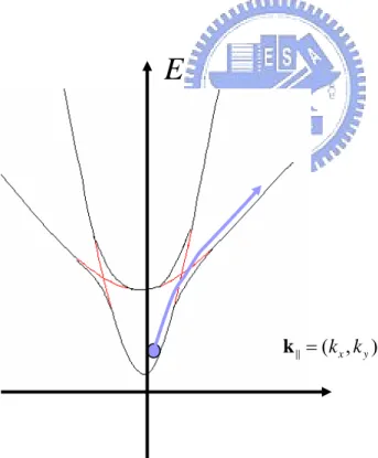
(10) 1. Introduction Recently, Terahertz laser has attracted much attention in many aspects. The spectrum indicates that the terahertz regime overlaps with a significant part of the molecular lines. Hence, these radiations can be used to detect and to interact with most molecules. Due to these features, the relevant physics and technologies are important to medical diagnosis, agriculture, water resource, environmental protection, etc. However, a convenient and inexpensive terahertz radiation source has not been available. The Gunn effect, namely the negative differential resistance, was first discovered by Gunn in 1963[1]. The mechanism responsible for the negative differential resistance of general oscillators, such as Gunn diodes, is a field-induced transfer of conduction-band electrons from high-mobility valley to low mobility valley [2]. The period of oscillation is the carrier transit time across the sample and the frequency of oscillation is equal to the reciprocal of the period of oscillation. Therefore, the frequency of oscillation would increase with decreasing the channel length. However, since the transfer of electrons between different valleys needs a large amount of electron-phonon interaction, when the channel length is not long enough, this process would be restricted by the electron-phonon interaction. Here we will present a mechanism where there is no need for electron-phonon interaction. Let us consider a heterostructure comprising GaAs and AlAs layers grown on the (001) plane. In such a heterostructure, because GaAs is a direct-bandgap material and AlAs is an indirect-bandgap material, the GaAs layers constitute potential wells for Γ-valley electrons and barriers for X-valley electrons, while the AlAs layers constitute potential wells for X-valley electrons and barriers for Γ-valley electrons (Fig 1). At the appropriate length of GaAs and AlAs layers, the Γ subband is higher than the X subband, and the Γ subband would meet X subband [3]. If Γ subband mixes with X subband, the two subbands constitute two Γ-X mixed subbands. Under the effect of the electric field, the Γ-valley electrons with low effective mass transfer to X valley with high effective mass (Fig 2). We can see that the scope of the band in Fig 2 decreases after Γ-X mixing, and this phenomenon is the negative differential resistance. This mechanism is not restricted by the 1.

(11) electron-phonon interaction. Therefore, the oscillation frequency is dominated by the channel length.. Fig 1 The band profile of the double-barrier heterostructure. E. k = (k x , k y ). Fig 2 The electron energy levels of the double-barrier heterostructure. 2.

(12) 2. Theory. Bulk evanescent states play an important role in determining the electronic properties of heterostructures. Several methods such as k ip model, tight-binding model, and empirical pseudopotential can be used to obtain bulk complex band structures. The total wave function is expanded in terms of bulk propagating and evanescent states on both sides of a matching plane. However, in the present system, since AlAs is an indirect-bandgap material, only considering the Γ symmetry point is not sufficient. It follows that the electronic properties of GaAs/AlAs heterostructures cannot be treated by usual approach, namely the k ip model. The restriction of this approach is that it requires wave vectors lying close to particular band extreme. In order to retain the multi-state property, empirical pseudopotential is used. Compared to the envelope-function approach, this method is valid for wave vectors throughout the first Brillouin zone. GaAs and AlAs are lattice-matched materials so that strain is not taken into account. The system is treated in the flat-band approximation. It is divided into several sections of alternative GaAs and AlAs. Each section is treated as quasi-bulk-like. The electronic wave function obtained from this method contains both the evanescent states and the Bloch states originating from various conduction-band minima.. 3.

(13) 2.1 Calculation of complex band structures [4],[5],[6] We start with the one-electron Schrödinger equation for a bulk-crystal of material j ⎡⎣ −∇ 2 + V j ( r ) + U 0j ⎤⎦ ϕ j ( r ) = Eϕ j ( r ). (2.1). The constant U 0j is to account for the band offset parameters between the respective material layers. At given E and k , the Bloch function can be expanded in terms of plane waves [4],[5], i.e.. ϕ j ( r ) = eik ⋅ru j ( r ) = eik ⋅r ∑ C ( k j , G )eiG⋅r j. j. (2.2). G. where G are reciprocal-lattice vectors. The Schrödinger equation written in the plane-wave basis is. ∑H. ( k )C ( k j. G ,G ′. j. , G′ ) = 0. (2.3). G. where 2 H G ,G ′ ( k j ) ≡ ⎡ ( k j + G ) − E ⎤ δ G ,G ′ + V ( G − G ′ ) ⎣ ⎦. (2.4). with V ( G − G′ ) being the pseudopotential form factors [7]. The H matrix is a quadratic polynomial in k z for fixed k j and E . Equation (2.4) can present in the form of H ( k j ) = H (0) ( k j ) + H (1) ( k j ) k z + k z ⋅ 1 2. 4. (2.5).

(14) where. (. ). H (0) ( k j ) = k j + G 2 + 2k j ⋅ G − E δ G ,G′ + V ( G − G′ ) 2. H k = 2Gzδ G ,G′ (1). (2.6). j. Equation (2.4) can be transformed into an eigenvalue equation for k z , i.e. 0 1 ⎡ ⎤⎡ C ⎤ ⎡C ⎤ ⎢ − H (0) k j − H (1) k j ⎥ ⎢ (1) ⎥ = k z ⎢ (1) ⎥ ( ) ( ) ⎦ ⎣C ⎦ ⎣C ⎦ ⎣. (2.7). where C (1) ≡ k z C . After diagonalizing the left first matrix of equation (2.7), we obtain the eigenvalues and corresponding eigenvectors. If N plane waves are used, there are 2 N solutions (which will be labeled with index s ). However, only the in-zone solutions should be retained, the number of which equals 2 M , where M is the number of projected reciprocal lattice vectors G . The general wave function in each layer j can be written as a linear combination of all Bloch-type solutions with different k zj ,s 2M. ψ j ( r ) = ∑ α j ,sϕ j ,s ( r ). (2.8). s. where ϕ j ,s ( r ) is given by equation (2.2).. 5.

(15) 2.2 Boundary conditions [6] This section will present the method to decide α j ,s in equation (2.8). The method is based on the theory of scattering matrix method, which can avoid numerical problems. Equation (2.2) can be transformed into the following form. ϕ j ,s ( r ) = eik ⋅r eik u j ,s ( r ) j ,s z. u j ,s ( r ) = ∑ Ak ,G eiG⋅r =∑ e G. G. = ∑∑ e G. iG ⋅r. iG ⋅r. Gz. ⎡⎣ Ak ,G eiGz z ⎤⎦. (2.9). ⎡⎣ Ak ,G eiGz z ⎤⎦ =∑ eiG ⋅r ∑ ⎡⎣ Ak ,G eiGz z ⎤⎦ Gz. G. From equation (2.8), the wave function in each layer j is now. ψ. j. ( r ) = ∑α j ,s eik ⋅r eik. j ,s z. s. = ∑e. i ( k + G )⋅r. = ∑e. i ( k + G )⋅r. G. G. ∑α s. ⎡ ⎤ iG ⋅r Ak j , s ,G eiGz z ⎥ ⎢∑ e ∑ z Gz ⎢⎣ G ⎥⎦ j ,s. ⎡ i ( k zj , s +Gz ) z ⎤ ⎤ ⎢ ∑ ⎣⎡ Akzj , s ,G e ⎦⎥ ⎣ Gz ⎦. ⎡ j ,s ⎡ i ( k zj , s +Gz )( z − z j ) ⎤ i ( k z′ j , s + Gz )( z − z j +1 ) ⎤ ⎤ j ,s ⎡ ′ e a A e b A + j ,s j ,s ∑s ⎢ ∑ ∑ ⎣ kz ,G ⎦ ⎣ kz′ ,G ⎦ ⎥⎦ Gz Gz ⎣ (2.10). where a j ,s and b j ,s are the coefficients of the “forward” and the “backward” state, respectively, with the forward states defined as those which propagate or exponentially decay in the positive-z direction and the backward states similarly defined as those which propagate or exponentially decay in the negative-z direction. z j and z j +1 are the left and right boundaries of each layer j .. 6.

(16) The boundary condition follow from demanding wave function and its first derivative to be continuous at the interface (located at z j +1 ). From equation (2.10), we can see that this condition can only be achieved when the coefficients of each G are equal, i.e.,. ⎡ ⎣. ∑ ⎢a ∑[ A s. j ,s. Gz. k zj ,s ,G. e. ⎡ = ∑ ⎢ a j +1,s ∑ [ Ak s ⎣ G. i ( k zj ,s + Gz )( z j +1 − z j ). ⎡ ⎣. s. j ,s. Gz. k zj ,s ,G. ⎡ = ∑ ⎢ a j +1,s ∑ [ Ak s ⎣ G. z. Gz. j +1,s ,G z. ] + b j +1,s ∑ [ Ak′′ Gz. z. ∑ ⎢a ∑[ A. ] + b j ,s ∑ [ Ak′′. (k zj ,s + Gz )e. z. j +1,s. ,G. e. i ( k zj ,s + Gz )( z j +1 − z j ). j ,s. ,G. ⎤ ]⎥ ⎦. i ( k z′ j +1,s + Gz )( z j +1 − z j + 2 ). ] + b j ,s ∑ [ Ak′′ Gz. j +1,s ,G z. (k zj +1,s + Gz )] + b j +1,s ∑ [ Ak′′ Gz. z. z. j +1,s. z. ⎤ ]⎥ ⎦. j ,s. ,G. ⎤ (k z′ j ,s + Gz )]⎥ ⎦. (k z′ j +1,s + Gz )e ,G. i ( k z′ j +1,s + Gz )( z j +1 − z j + 2 ). ⎤ ]⎥ ⎦. (2.11) Equation (2.11) can be transformed into the matrix form, i.e., ⎡ a( n ) ⎤ ⎡ a( n+1) ⎤ ⎢ ( n ) ⎥ = T (n + 1) ⎢ ( n+1) ⎥ ⎣b ⎦ ⎣b ⎦. (2.12). where T (n + 1) is the transfer matrix. After separating the forward and backward states at the two sides of equation (2.12), we obtain equation (2.13), the scattering matrix [8]. ⎡ a( n ) ⎤ ⎡a ( n+1) ⎤ ⎢ ( n+1) ⎥ = S (n + 1) ⎢ ( n ) ⎥ ⎣b ⎦ ⎣b ⎦. (2.13). The above equation can extend to the following form. 7.

(17) ⎡ a( n ) ⎤ ⎡a ( m ) ⎤ ⎢ ( m ) ⎥ = S ( n, m ) ⎢ ( n ) ⎥ ⎣b ⎦ ⎣b ⎦. (2.14). where ⎡ S (n, m) S12 (n, m) ⎤ S (n, m) = ⎢ 11 ⎥ ⎣ S 21 (n, m) S22 (n, m) ⎦ a ( m ) = S11 (1, m)a(1) + S12 (1, m)b ( m ). (2.15). b ( m ) = S21 (m, N )a ( m ) + S 22 (m, N )b ( N ). The matrices Sij (n, m) depend on energy E and in-plane wave vector k . In order to calculate the energy state of the system, we set the vector coefficients a (1) and b ( N ) for the incoming waves to be zero. Therefore, the eigenvalue equation can be written as [9] [ I − S21 (m, N ) S12 (1, m)]b ( m ) = 0. (2.16). In such a GaAs/AlAs system, electron could escape from the system via Γ − Χ transfer; consequently the energy state should be complex so that it could represent its behavior varying with time, i.e.. ψ (r, t ) = e. E −i t. φ (r ) = e 2 Ei. 2. ∫ ψ (r, t ) dV = e. −. ∫ ψ (r, t ). 2. −. t. −. Ei. t −i. Er. e. t. 2. φ (r ), E = Er − i ⋅ Ei. ∫ φ (r) dV ∝ e. −. 2 Ei. t. (2.17). t. dV ∝ e , τ = τ. 2 Ei. In solving this nonlinear two-dimensional equation (2.16), the usual 2-D 8.

(18) Newton method is used. Only the solution with positive Ei has physical meaning. However, in some cases we cannot find the solutions. The problems might be from that we cannot find the appropriate initial guess close to the solutions. Still another method can be used. Solving equation (2.16) is equivalent to diagonalize S 21 (m, N ) S12 (1, m) with eigenvalue 1.. The eigenvalue of S 21 (m, N ) S12 (1, m) can be written as R ⋅ eiθ . R is approximately linear in Ei , since the amplitude represents the loss. θ is approximately linear in Er , since Er has the information of frequency, frequency is the reciprocal of wavelength, and wavelength has the information of phase. However, in some cases, we cannot find meaningful E . The problem is the same as 2-D Newton method. We have to find a powerful numerical method so that the analysis can be more complete. If in the case that we emphasize on the anticrossing gaps of the GaAs/AlAs heterostructures, we can only calculate Er , and Ei is not taken into account. The profiles of the two approaches are much the same.. 9.

(19) 2.3 Transmission coefficient Transmission coefficient is calculated from the definition of the current flux that T=. J transmit J incidnet. (2.12). * where J x = Re ⎡(ϕ j,s ) ( −i∇ϕ j,s ) ⎤ . Only the state with real k zj ,s can have ⎣⎢ ⎦⎥. nonzero current flux. The plot of E versus T can help us plot E versus k . At k = (0,0) , the peak of the plot E versus T is the resonance energy and can be classified into different types of quasi-bound states. The energy of quasi-bound states is in fact equal to the energy level of the system at that k . From curvature of the band we can classify the band into Γ or Χ quasi-bound state. Since the transverse effective mass of Χ valley is several times larger than the transverse effective mass of Γ valley, the curvature of Γ quasi-bound states would be larger than Χ quasi-bound states.. 10.

(20) 3. Simulation Results This chapter is divided to two sections. In the first section, the complex band structures of GaAs and AlAs are presented. The second section is the Γ − Χ mixing effect on the subband structure, where anticrossing gap is an important parameter. The logarithmic plots of transmission coefficients as a function of electron energy with k & = (0,0) are presented as well. The anticrossing gap is defined as the minimum energy separation between the mixed Γ − Χ states. Since we want intense Γ − Χ interaction so that the electrons of Γ -valley can easily transfer to Χ -valley under the applying of electric field in the parallel direction, we want to obtain a structure with a large anticrossing gap. In this chapter, GaAs is defined as the well material and AlAs is defined as the barrier material in the name of the Γ -valley electrons.. 11.

(21) 3.1 Complex band structures The empirical pseudopotential method is used to calculate the bulk complex band structure. The pseudopotential form factors can be adjusted as well to fit the particular band parameters. Note that a little change in the form factors would lead to large change in the band structure. Fig.1 and Fig.2 are the complex band structure of GaAs and AlAs respectively. The energy of conduction Γ -valley in GaAs is shifted to zero. The lowest conduction band in AlAs lies at the Χ -valley.. Fig 3 Complex band structure of GaAs along [001] direction. 12.

(22) Fig 4 Complex band structure of AlAs along [001] direction From Fig1. and Fig2., we can see that GaAs is a direct band gap material, and AlAs is an indirect band gap material. The X-valley of AlAs is at 0.1492 eV and the Γ -valley of GaAs is at 1.1048 eV. Therefore, AlAs is the barrier for the Γ -valley electrons, and GaAs is the barrier for the X-valley electrons. Thus, with specific length of each material, the Γ -valley electrons and X-valley electrons will confined at different material. The above phenomenon is the origin of Γ -X mixing effect.. 13.

(23) 3.2 Γ - Χ mixing effect on the subband structure Since only at the interface can electrons transfer from Γ -valley to X-valley, the interfaces play an important role in the Γ -X mixing effect. Therefore, we will discuss the effect of interface in two ways. The first one is that the total length of the heterostructure is fixed, and the length of one pair of a barrier and a well is changed. The second one is that the length of one pair of a barrier and a well is fixed, and the total length of the heterostructure is changed.. 14.

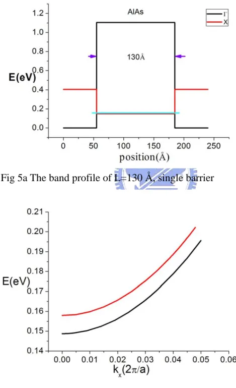
(24) Case 1. Total length of the heterostructure is fixed. 1. Total Length L=130 Å (1) Single barrier. Fig 5a The band profile of L=130 Å, single barrier. Fig 5b The subband structure of L=130 Å, single barrier. 15.

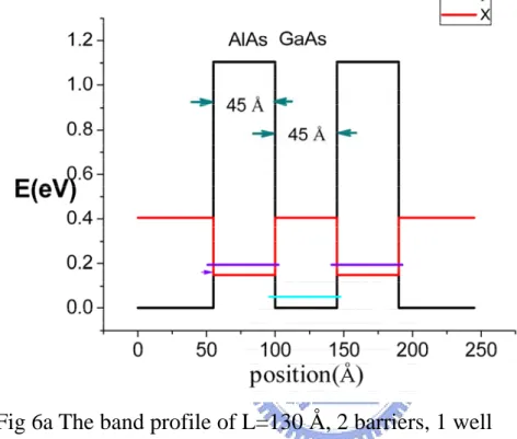
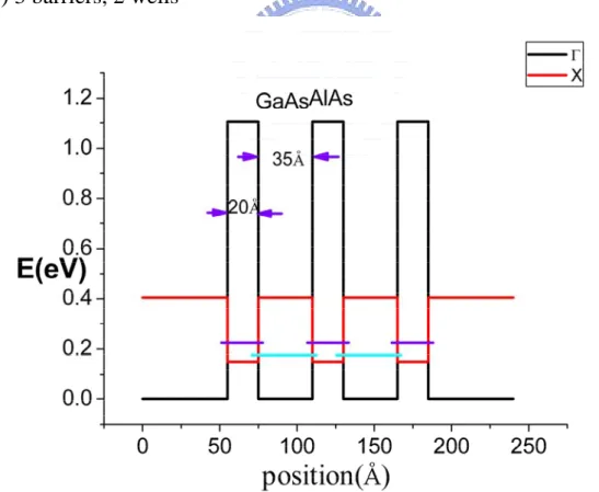
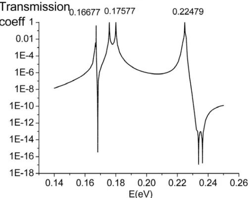
(25) In this structure, since there is no GaAs well to constitute Γ well, there is no Γ quasi-bound states to provide Γ -X mixing effect. Therefore, the subband structure monotonic increases with k x . (2) 2 barriers, 1 well. Fig 6a The band profile of L=130 Å, 2 barriers, 1 well. Fig 6b The logarithmic plot of transmission coefficient of L=130 Å, 2 barriers, 1 well. The incident state is the state with k & = 0 16.

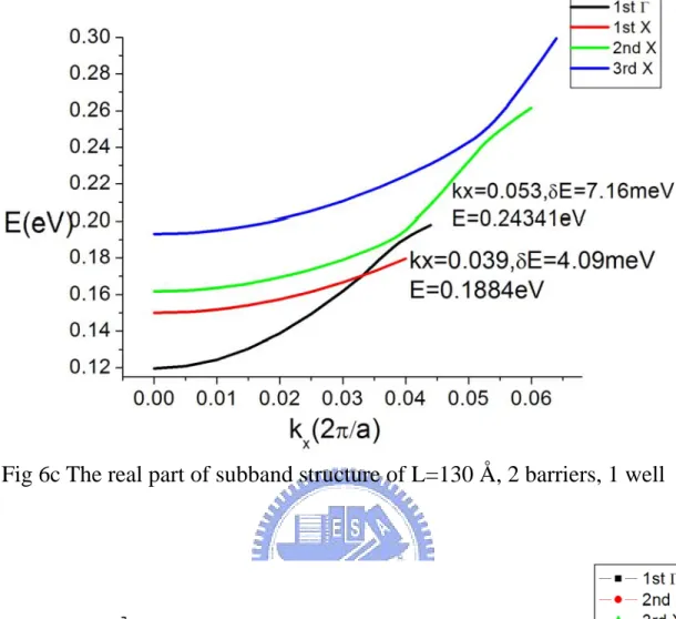
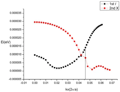
(26) Fig 6c The real part of subband structure of L=130 Å, 2 barriers, 1 well. Fig 6d The imaginary part of subband structure of L=130 Å, 2 barriers, 1 well 17.

(27) From Fig 4b, we can see four peaks, which correspond to four energy states, the quasi-bound states. The lowest energy state is the Γ state, which is confined at GaAs well and corresponds to the lowest subband in Fig 4c and has smaller curvature. The other three energy states correspond to X states, which correspond to the other three subbands in Fig4c and have the larger curvature. In Fig 4c, the lowest Γ state increases monotonically with k x , and when it meets with the second X state, the Γ -X mixing effect occurs, meaning that at this energy, the 2 wave functions have both the Γ and X part. After that, the original Γ state becomes the X state, and the original X state becomes the Γ state. We can see that the second anticrossing gap is larger than the first anticrossing gap. This is because when the energy is higher, the wave function is less localized; thus the overlap of the Γ and X wave functions is larger. (3) 3 barriers, 2 wells. Fig 7a The band profile of L=130 Å, 3 barriers, 2 wells. 18.

(28) Fig 7b The logarithmic plot of transmission coefficient of L=130 Å, 3 barriers, 2 wells. The incident state is the state with k & = 0. Fig 7c The real part of subband structure of L=130 Å, 3 barriers, 2 well 19.

(29) Fig 7d The imaginary part of subband structure of L=130 Å, 3 barriers, 2 wells From Fig 5c, we can see that the lowest subband is the X subband. The second subband is the Γ subband, and when it meets with the higher X subband, Γ -X mixing effect occurs. (4) Unsymmetrical structure, 2 barriers, 1 well. Fig 8a The band profile of L=130 Å, unsymmetrical structure, 2 barriers, 1 well 20.

(30) Fig 8b The logarithmic plot of transmission coefficient of L=130 Å, unsymmetrical structure, 2 barriers, 1 well. The incident state is the state with k & = 0. Fig 8c The real part of subband structure of L=130 Å, 2 barriers, 1 well 21.

(31) Fig 8d The imaginary part of subband structure of L=130 Å, 2 barriers, 1 well Compared with the result in (2), although the number of interfaces is the same, the anticrossing gap in (4) is smaller due to two reasons. The first one is that at the energy which Γ − Χ mixing occurs is lower in (4); thus the Γ and X wave functions are more localized. Therefore, the overlap of the wave functions is weaker. The second one is that when Γ − Χ mixing effect occurs, the X wave function almost localizes at one AlAs barrier, since the two barriers are unsymmetrical. This is like the case with only one AlAs barrier.. 22.

(32) 2. Total Length L=215 Å (1) 3 barriers, 2 wells. Fig 9a The band profile of L=215 Å, 3 barriers, 2 wells. Fig 9b The logarithmic plot of transmission coefficient of L=215 Å, 3 barriers, 2 wells. The incident state is the state with k & = 0. 23.

(33) Fig 9c The subband structure of L=215 Å, 3 barriers, 2 wells. (2) 4 barriers, 3 wells. Fig 10a The band profile of L=215 Å, 4 barriers, 3 wells. 24.

(34) Fig 10b The logarithmic plots of transmission coefficient of L=215 Å, 4 barriers, 3 wells. The incident state is the state with k & = 0. Fig 10c The subband structure of L=215 Å, 4 barriers, 3 wells. 25.

(35) Case 2. Total length of one pair of a barrier and a well is fixed. 1. BL=30Å, WL=35Å (1) 2 barriers, 1 well. Fig 11a The band profile of BL=30 Å, WL=35 Å. (2 barriers, 1 well). Fig 11b The subband structure of BL=30 Å, WL=35 Å. (2 barriers, 1 26.

(36) well) (2) 4 barriers, 3 wells. Fig 12a The band profile of BL=30 Å, WL=35 Å. (4 barriers, 3 well). Fig 12b The subband structure of BL=30 Å, WL=35 Å. (4 barriers, 3 wells) 27.

(37) 2. BL=45Å, WL=45Å (1) 2 barriers, 1 well. Fig 13a The band profile of BL=45 Å, WL=45 Å. (2 barriers, 1 well). Fig 13b The subband structure of BL=45 Å, WL=45 Å. (2 barriers, 1 well) 28.

(38) (1) 3 barriers, 2 wells. Fig 14a The band profile of BL=45 Å, WL=45 Å. (3 barriers, 2 wells). Fig 14b The subband structure of BL=45 Å, WL=45 Å. (3 barriers, 2 wells). 29.

(39) Case 1: Total length of the structure is fixed. Total Length L=130 Å Structure. 1st Anticrossing Gap 2nd Anticrossing Gap (meV) (meV) 0 0 4.09 7.16 18.28 2.47. 1 barrier 2 barriers, 1 well 3 barriers, 2 wells Unsymmetrical, 2 barriers, 1 well Table 1 Anticorssing gap. Total length of the structure is fixed. L=130 Å Total Length L=215 Å Structure 3 barriers, 2 wells. 1st Anticrossing Gap 2nd Anticrossing Gap (meV) (meV) 4.76 7.72. 4 barriers, 3 wells 11.86 Table 2 Anticorssing gap. Total length of the structure is fixed. L=215 Å. Case 2: The Length of one pair of a barrier and a well is fixed. BL=30 Å, WL=35 Å Structure Anticrossing Gap (meV) 2 barriers, 1 wells 12.56 4 barriers, 3 wells 11.86 Table 3 Anticorssing gap. Length of one pair of a barrier and a well is fixed. BL=30 Å, WL=35 Å BL=35 Å, WL=35 Å Structure Anticrossing Gap (meV) 2 barriers, 1 wells 4.09 3 barriers, 2 wells 3.79 Table 4 Anticorssing gap. Length of one pair of a barrier and a well is 30.

(40) fixed. BL=35 Å, WL=35 Å First of all, let’s consider case 1. From Table 1, we can see that when the total length of the structure is fixed, the anticrossing gap increases with the number of the interfaces per unit length. This is because the interface dominates the Γ - Χ mixing effect. Therefore, when the total length of the structures is fixed, the increase of the number of the interface would lead to stronger Γ - Χ mixing effect. In the same structure, the second anticrossing gap is larger than the first anticrossing gap, since the larger the energy state is; the less localized the wave function is. Compare the result in the second row and the fourth row of the Table 1, and the anticrossing gap of the unsymmetrical structure is smaller than that of the symmetric one, although the two structures have the same number of interfaces. This is because when Γ - Χ mixing effect occurs, the energy states of the two divided GaAs wells are different. Therefore, this is like the case that only one AlAs well can contribute to the Γ - Χ mixing effect. The result of the Table 2 can be explained by the above discussion. Second, let’s consider case 2. The length of the one pair of a barrier and a well fixed means that the number of interfaces per unit length is fixed. The change of the anticrossing gap is much smaller than that of the case 1. This is due to two reasons. First, the energy states of the first row and the second row in the Table 3 and Table 4 are almost the same. Therefore, the overlap of the Γ and Χ wave functions is almost equal. Second, the number of the interfaces per unit length is the same, which is the same as the discussion in case 1. Finally, we can conclude that the dominant factor of the anticrossing gap is the number of the interfaces per unit length, not the number of the interfaces. Consequently, with the purpose of large anticrossing gap, the increase of the number of the interfaces per unit length and a symmetric structure is necessary.. 31.

(41) 4. Conclusion This thesis proposed a novel idea to realize the terahertz laser which is based on the mechanism of negative differential resistance. The proposed structure utilizes the Γ - Χ mixing effect to produce negative differential resistance. Therefore, the oscillation frequency is dominated by the channel length and will not be restricted by the electron-electron scattering rate. The structure is simple and easy to fabricate in the present technology. The phononless intervalley scattering at the interface cannot be taken into account by the usual effective-mass theory. Therefore, empirical pseudopotential is used to calculate the complex band structure, which is the appropriate candidate to obtain multi-state properties for Γ - Χ mixing effect. Besides, scattering matrix method can treat a large system as well without any numerical problems. The proper structure is with the large anticrossing gap. The first requirement is a symmetric structure. Moreover, the dominate factor is the number of the interfaces per unit length, not the total number of the interfaces.. 32.

(42) [1] J. B. Gunn, “Microwave Oscillation of Current in III-V Semiconductors,” Solid State Commun., 1, 88 (1963) [2] S. M. Sze, “Physics of Semiconductor Devices”, 2nd ed., p637. [3] D. Z. –Y. Ting, Yia-Chung Chang, “Γ-X mixing in GaAs/AlxGa1-xAs/AlAs superlattices”, Phys. Rev. B 36, 4359 (1987) [4] Marvin L. Cohen, T. K. Bergstresse, “Band Structures and Pseudopotential Form Factors for Fourteen Semiconductors of the Diamond and Zinc-blende Structures”, Phys. Rev. 141, 789 (1966) [5] Yia-Chung Chang, J. N. Schulman, “Complex band structures of crystalline solids: An eigenvalue method”, Phys. Rev. B 25, 3975 (1982) [6] J P Cuypers, W van Haeringen, “Matching of electronic wavefunctions and envelope functions at GaAs/AlAs interfaces”, J. Phys.: Condens. Matter 4, 2587 (1992) [7] Jian-Bai Xia, “Γ-X mixing effect in GaAs/AlAs superlattices and heterojunctions” , Phys. Rev. B 41, 3117 (1990) [8] David Yuk Kei, J. C. Inkson, “Matrix method for tunneling in heterostructures: Resonant tunneling in multilayer systems”, Phys. Rev. B 38, 9945 (1988) [9] A. Zakharova, S. T. Yen, K. A.Chao, “Hybridization of electron, lighthole and heavy-hole states in InAs/GaSb quantum wells”, Phys. Rev. B 64,233532 (2001). 33.

(43)