Integration of Background Modeling and Object Tracking

INTEGRATION OF BACKGROUND MODELING AND OBJECT TRACKING

Yu-Ting Chen

_{, Chu-Song Chen}

_{, and Yi-Ping Hung}

_{Institute of Information Science, Academia Sinica, Taipei, Taiwan.}

2

_{Dept. of Computer Science and Information Engineering, National Taiwan University, Taipei, Taiwan.}

_{Graduate Institute of Networking and Multimedia, National Taiwan University, Taipei, Taiwan.}

ABSTRACT

Background model and tracking became critical components for many vision-based applications. Typically, background modeling and object tracking are mutually independent in many approaches. In this paper, we adopt a probabilistic framework that uses particle filtering to integrate these two approaches, and the observation model is measured by Bhat-tacharyya distance. Experimental results and quantitative eval-uations show that the proposed integration framework is ef-fective for moving object detection.

1. INTRODUCTION

Background modeling/subtraction is a fundamentally impor-tant module for many applications, such as visual surveillance and human gesture analysis. By learning a background model from a training image sequence, the problem of moving object detection is transformed to that of classifying a static scene into foreground and background regions.

Methods of background modeling are mainly studied in pixel level and statistical distribution of each individual pixel is usually modeled by Gaussian distribution. Generally, a sin-gle Gaussian model used in [12] and [5] is not sufficient to represent the background since the backgrounds is often non-stationary. In [10], Stauffer and Grimson proposed a state-of-the-art framework, Mixture of Gaussian (MoG), to modeled each pixel with k Gaussians, where k lies in 3 to 5, and an on-line K-means approximation was used instead of using exact EM. Besides, the MoG approach is modified or extended in several researches. For example, [3] and [4] used YUV color plus depth and Local Binary Pattern (LBP) [9] histogram as features, respectively. In [8], Lee proposed an effective learn-ing algorithm for MoG. Instead of uslearn-ing Gaussian mixtures, several other methods adopted different models. For exam-ple, Toyama et al. [11] proposed a Wallflower framework to address the background maintenance problem in three levels, pixel, region, and frame levels. In [2], Elgammal et al. pro-posed a non-parametric background subtraction method uti-lizing Parzen-window density estimation. In [7], Kim et al. presented a real-time algorithm called CodeBook that is effi-cient in either memory or speed.

After moving object is detected by background model-ing, some tracking algorithms might be performed to track the object. Typically, there are two mechanisms, appearance model and search algorithm, for object tracking. For exam-ple, MeanShift [1] used color histogram as the appearance model to measure the similarity of the target object and can-didates. On the other hand, the search algorithm finds the most likely state of the tracked object according to its simi-larity measurement. For example, Isard and Blake proposed CONDENSATIONalgorithm [6] to track the contour of object.

In previous researches, background modeling and object tracking are usually performed independently to each other. Actually, good detection result of background modeling can provide good prior information for tracking. On the contrary, good tracking results might be a better prior knowledge for adjusting the background models. In this paper we provide a framework to integrate and cooperate background modeling and object tracking approaches with the use of probabilistic framework.

To integrate these two approaches, recall that each incom-ing image is classified into foreground and background re-gions by learned background model. To do this, the feature of each pixel of incoming image is compared against existing background models until a match is found. A match is defined as the distance between feature and learned model is less than a threshold T . If a matched model is found and is a stable model (see Section 2), the pixel is detected as background; otherwise, the pixel is classified as foreground. Typically, the threshold T is usually kept as a static variable in previous researches. Based on the following two observations, the se-lection of T is not easy:

• When the color of moving object is similar to that of

the background, a strict T is preferred to prevent fore-ground object from being classified as backfore-ground.

• When the color of moving object is dissimilar to that of

the background, a loose T is suitable to decrease false alarm (background regions are detected as foreground). On the basis of these two observations, we address the problem of variable threshold selection for background mod-eling. In this paper, color histogram of object is used as

ap-pearance model for object tracking and the tracking result is used to select a discriminative T to separate input image into foreground and background regions with maximum separabil-ity. In addition, such adjusted background model can provide better detection result as a prior for tracking.

In this paper, our contribution is that a probabilistic frame-work uses particle filtering to integrate background modeling and object tracking, and the observation model is measured by Bhattacharyya distance as used in [1]. In addition, existing background approaches can be adopted with merely a slight modification and MoG [10] approach is used in this work. Ex-perimental results and quantitative evaluations show that the proposed integration framework is effective for moving object detection.

2. GENERAL DESCRIPTION OF BACKGROUND MODELING

A pixel-based approach can be generally characterized as a quadruple {F, M(t), Φ, Γ}. The first element F depicts the

feature extracted for a pixel, which might be gray/color val-ues [2, 3, 7, 10], depth [3], etc. The second element M(t)

consists of the background models maintained at time t for the pixel, e.g. each model in MoG is represented as a single Gaussian distribution in the mixture. Note that almost all the methods maintained M(t) = {M(t)S , M(t)P}, where M(t)S and

MP

(t)are the sets of stable and potential background models,

respectively. For example, in MoG [10], the first B Gaussian densities constitute MS

(t) and the other constitute M(t)P. In

CodeBook [7], background model and cache model stand for

MS

(t)and M(t)P, respectively. The third element Φ is a function

determining whether a given pixel q at time t is background based on pixel feature, stable background models, and thresh-old:

{1, 0} ← Φ[F (q), MS

(t), T ], (1)

where F (q) is the feature of q, T is the threshold for finding out the matched model in MS

(t), and 1 and 0 stand for

back-ground and foreback-ground respectively. Note that only the stable model MS

(t) is involved in the determination. To realize Φ

typically involves the search of the matched model in MS (t).

That is, the distance between matched model and F (q) is less than T . The fourth element Γ is another function that updates the model and generate a new model at time t + 1 based on pixel feature F (q), current model M (t), and threshold T :

M(t+1)← Γ[F (q), M(t), T ], (2)

and a new pair of models, M(t+1) = {M(t+1)S , M(t+1)P }, is

obtained. To realize Γ typically involves the search of the matched model to F (q) in M(t).

Note that in Eq. (1), if no matched model is found, the corresponding pixel is determined as foreground; otherwise the pixel is background. Therefore, more false positive and more false negative results are obtained with the use of strict

and loose T , respectively. In previous researches, the value of T is usually defined as a static variable. To our knowl-edge, no research has used variable T . In this framework, particle filtering is used to select a suitable T according to object tracking result. Besides, our approach does not restrict adopted background modeling approach, and MoG is used in this work.

3. VARIABLE THRESHOLD SELECTION After background model is learned, an initial value is selected for T . In our experiment, we choose initial T as 3 in MoG model. Once a moving object is detected at time t, the track-ing algorithm is started and the color histogram Ot of

de-tected object in foreground region R is calculated. To com-pute Ot, let {uji}i=1,...,n;j∈{R,G,B} be the intensity value at

color channel j of the pixel u located at i of incoming im-age It. We use 16 bins to calculate the intensity histogram

for each color channel j. Therefore, the color histogram has

K = 48(16 × 3 = 48) bins. Besides, we define a function b : uj_i → {1, . . . , K} which maps uj_i to the bin index b(uj_i) of the histogram, and the color histogram Otis calculated by

Ot(k) = C

X

ui∈It;ui∈R

δ[b(uj_i) − k], (3)

where C is a normalization term to ensurePK_k=1Ot(k) = 1

and δ is the Kronecker delta function. With the appearance information Ot, the object can be tracked by measuring the

similarity of Otand color histogram of candidates at time t +

1. In addition, particle filtering with prior information of Otis

used to choose discriminative threshold T . In the following, we briefly introduce particle filtering and adopted dynamic model and observation model.

3.1. Particle Filtering

Particle filtering is based on Bayesian Approach and Mote Carlo Sequential Method, and the main concept is captured by CONDENSATION[6]. For simplicity, we use formulation

of CONDENSATIONto briefly describe the particle filtering.

Let state parameter vector at time t be denoted as xt, and

its observation as zt. The history of state parameters and

ob-servations from time 1 to t is denoted as Xt= {x1, . . . , xt}

and Zt= {z1, . . . , zt}, respectively. Particle filtering is used

to approximate posterior distribution of state xt+1given

ob-servation Zt+1. From Bayesian rule and Markov chain with

independent observations, the rule for propagation of poste-rior over time is:

p(xt+1|Zt+1) ∝ p(zt+1|xt+1)

Z

xt

p(xt+1|xt)p(xt|Zt).

(4) Note that the recursive form allows the posterior at time

p(xt+1|Zt+1) by a finite set of N particles St= {s(n)t , π (n) t },

where stis a value of state xtand πtis a corresponding

sam-pling probability. Besides, dynamic model, p(xt+1|xt), and

observation model, p(zt+1|xt+1), are needed and we will

de-scribe our choice of these two probabilities in the following subsection. More details and theoretical foundation can be found in [6]. One iteration steps are shown below:

1. Select samples S0

t= {s0(n)t , π 0(n)

t } from St.

2. Predict by sampling from s(n)_t+1 = p(xt+1|xt = s0(n)t )

and π(n)_t+1= 1/N .

3. Measure and weight π_t+1(n) in terms of the measured fea-ture zt+1as: πt+1(n) = p(zt+1|xt+1= s(n)t+1).

4. Normalize π_t+1(n) such thatPπ(n)_t+1= 1. 3.2. Variable Threshold Selection

To select T , particle filtering is used and N particles are sam-pled with all stand πtare initialized as 3 and 1/N ,

respec-tively. Recall that we need to define the dynamic model and observation model for particle filtering.

3.2.1. Dynamic Model

An unconstrained Brownian motion is used as dynamic model: s(n)t+1= s0(n)t + vt, (5)

where vt∼ N (0, Σ) is a normal distribution. 3.2.2. Observation Model

To begin with, the reference background image Reftshall be

calculated from background model M(t). In our experiments,

we use the mean of most stable Gaussian model (with maxi-mum σ/ω value in MoG) to represent the pixel value of image

Reft. In time step t + 1, input frame image It+1can be

classi-fied into foreground region R(n)_{F G}and background region R(n)_BG by assigning T = s(n)_t+1for each particle.

Therefore, two color histograms, IF G

t+1and It+1BG, of

fore-ground and backfore-ground regions of image It+1and one color

histogram, RefBG

t , of background region of image Reftcan

be calculated by: It+1F G(k) = C1 X ui∈It+1;ui∈R(n)F G δ[b(uj_i) − k], (6) IBG t+1(k) = C2 X ui∈It+1;ui∈R(n)BG δ[b(uj_i) − k], (7) and RefBG_t (k) = C3 X ui∈Reft;ui∈R(n)BG δ[b(uj_i) − k], (8)

where C1, C2, and C3are all normalization terms.

With the use of discriminative threshold T , the color his-togram of tracked object is similar to that of the foreground region of image It+1, and the color histogram of background

region of image Reftis similar to that of background region

of image It+1. That is, Ot and RefBGt are similar to It+1F G

and IBG

t+1respectively, and Bhattacharyya distance is used to

measure the similarity between two histograms h1and h2:

dist(h1, h2) =

qPK i=1

p

h1(i)h2(i), (9)

where h1(i) and h2(i) are ithbin value of h1and h2.

There-fore, two distances, dist(Ot, It+1F G) and dist(RefBGt , It+1BG) can

be calculated. The observation model is defined as the linear combination of these two distances as:

π_t+1(n) = p(zt+1|xt+1= s(n)t+1) (10)

= α × dist(Ot, It+1F G) + (1 − α) × dist(RefBGt , It+1BG),

where 0 ≤ α ≤ 1 is a user defined parameter and we set

α = 0.5 in our experiments.

Once all N patricles are measured, the threshold T at time step t+1 is selected as s(n)_t+1whose corresponding π_t+1(n)has the maximum sampling probability over all N particles. Image

It+1 can then be classified into foreground and background

according to T . Finally, IF G

t+1is calculated and used for

updat-ing the color histogram of tracked object for robust trackupdat-ing in time step t + 2 as:

Ot+1(i) = β Ot(i)+(1−β) It+1F G(i) (i = 1, . . . , K), (11)

where 0 ≤ β ≤ 1 is a user defined parameter and we set

β = 0.8 to 0.95 in our experiments.

4. EXPERIMENTAL RESULTS

To evaluate proposed method, one outdoor and one indoor video sequences of the ATON project (http://cvrr.ucsd.edu/ aton/shadow) are adopted as the benchmarks as summarized in Table 1. These two sequences of ATON include outdoor

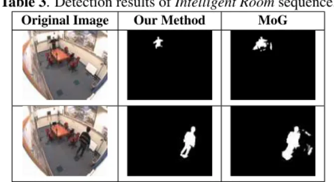
Campus sequence with signal noises and static indoor Intel-ligent Room sequence. Detection results of our method with

10 particles and original MoG are shown in Table 2 and 3, respectively. From these results, our method with variable T has generally better results than original MoG method.

Besides, we use false positive (background pixels are clas-sified as foreground), false negative (foreground pixels are classified as background), and the summation of false posi-tive and false negaposi-tive to quantitaposi-tively evaluate the effect of our method. The post processing and all parameter for our method and MoG are set the same and the evaluation results are shown in Table 4. Table 4 shows that proposed method can provide an averagely low error classified number of pix-els of background modeling. In addition, the average speed of Campus and Intelligent Room sequences are 5.30 fps and 8.22 fps by using 3.4 GHz processor and 768 MB memory.

Table 1. Two benchmark sequences used in our experiments.

Sequence Name Campus Intelligent Room

Sequence Image

Frame Number 400 170

Sequence Type Outdoor Indoor

Image Size 320×240 320×240

Frames for Training 20 20

Table 2. Detection results of Campus sequence.

Original Image Our Method MoG

5. CONCLUSION

A method for integrating background modeling and object tracking is presented in this paper. In this framework, color histogram of moving object is used as appearance model for object tracking. Besides, the tracking result is used to se-lect a discriminative threshold T for background modeling via particle filtering. Experimental results show that the pro-posed framework can further improve the performances of the adopted background modeling approach.

ACKNOWLEDGMENTS: This work was supported in part under grants NSC 94-2752-E-002-007-PAE and 94-EC-17-A-02-S1-032.

6. REFERENCES

[1] D. Comaniciu, V. Ramesh, and P. Meer, “Real-time Tracking of Non-rigid Objects using Mean Shift,” Proc. CVPR, 2000. [2] A. Elgammal, D. Harwood, and L. S. Davis, “Non-parametric

Model for Background Subtraction,” Proc. ECCV, 2000. [3] M. Harville, “A Framework for High-level Feedback to

Adap-tive, Per-pixel, Mixture-of-Gaussian Background Models,”

Proc. ECCV, 2002.

[4] M. Heikkil¨a and M. Pietik¨ainen,“A Texture-based Method for

Table 3. Detection results of Intelligent Room sequence.

Original Image Our Method MoG

Table 4. Quantitative evaluations by averaged false positive (FP), false negative (FN), and the summation of FP and FN.

Sequence

Name Algorithm FP FN FP+FN

Campus Our Method 133.37 124.68 258.05

MoG 364.16 34.47 398.63

Intelligent Our Method 426.33 114.44 540.77

Room MoG 563.56 63.78 627.34

Modeling the Background and Detecting Moving Objects,”

IEEE Trans. on PAMI, 28(4), 2006.

[5] T. Horprasert, D. Harwood, and L. S. Davis, “A Statistical Approach for Real-time Robust Background Subtraction and Shadow Detection,” Proc. ICCV Frame-rate Workshop, 1999. [6] M. Isard and A. Blake, “Contour Tracking by Stochastic

Prop-agation of Conditional Density,” Proc. ECCV, 1996.

[7] K. Kim, T. H. Chalidabhongse, D. Harwood, and L. S. Davis, “Real-time Foreground-Background Segmentation Us-ing CodeBook Model,” Real-Time ImagUs-ing, 11(3), 2005. [8] D. S. Lee, “Effective Gaussian Mixture Learning for Video

Background Subtraction,” IEEE Trans. on PAMI, 27(5), 2005. [9] T. Ojala, M. Pietikainen, and T. Maenpaa, “Multiresolution Gray-scale and Rotation Invariant Texture Classification with Local Binary Patterns,” IEEE Trans. on PAMI, 24(7), 2002. [10] C. Stauffer and W. E. L. Grimson, “Adaptive Background

Mix-ture Models for Real-time Tracking,” Proc. CVPR, 1999. [11] K. Toyama, J. Krumm, B. Brumitt, and B. Meyers,

“Wall-flower: Principles and Practice of Background Maintenance,”

Proc. ICCV, 1999.

[12] C. R. Wren, A. Azarbayejani, T. Darrell, and A. P. Pent-land, “Pfinder: Real-time Tracking of the Human Body,” IEEE