iCare:社群化智慧型居家照護－子計畫二：感測網路於居家照護之應用(3/3)

行政院國家科學委員會專題研究計畫 成果報告

iCare:社群化智慧型居家照護--子計畫二：感測網路於居

家照護之應用(3/3)

研究成果報告(完整版)

中 華 民 國 97 年 02 月 22 日

行政院國家科學委員會專題研究計畫 結案報告 感測網路於居家照護之應用 (3/3)

Sensor Network for Home Care (3/3) 計畫編號：NSC 95-2218-E-002 -024 執行期間：95 年 10 月 1 日 至 96 年 9 月 31 日 (第三年) 執行單位：國立台灣大學電機工程學系暨研究所 計畫主持人：黃寶儀 計畫參與人：吳瑞傑、劉承榮、蕭俊杰、陳星豪、吳意曦、林宗翰 一、中英文摘要 感測器(sensor)與無線感測網路(sensor network) 的研究及技術逐漸成熟，使其在 智慧型系統的應用上受到廣泛的注目。智慧型系統可以利用感測網路收集到的環 境參數，達成使用者與系統間輕鬆且聰明的互動。未來幾年，無線感測網路的發 展將大幅推進至諸如軍事、工業、生態環境研究等方面的應用。因應現今社會人 口老化，慢性疾病人口增加的趨勢，本計畫特別著眼於無線感測網路在智慧型居 家照護(intelligent home care) 上的應用。在這個應用領域，無線感測網路扮演了 收集老人居家生活情形中各種參數的重要角色。

有別於目前的技術，無線感測網路用於居家照護的設計上有三個特點：固定與行 動節點並存、資料種類的多樣、及感測資料傳達的即時性。在設計創新及技術轉 移可行性並重的前提下，我們提出了（一）adaptive diffusion 、（二）fast content-based forwarding 、及（三）two-class service differentiation 來因應前列三 項特性的需要。Adaptive diffusion 是一個以資料為中心的調整型路由機制。Fast content-based forwarding 可 望 解 決 比 對 資 料 內 容 的 速 度 問 題 。 Service differentiation 則增加即時資料取得的可靠與容錯性。我們的目標是在三年內進 行整體計劃的評估、實作、與整合，並期領先全球完成無線感測網路於智慧型居 家照護的應用及實作。研究成果將奠定台灣在無線感測網路於一般消費市場研究 與應用的全球策略性地位，並開創System on Chip (SOC) 在，以感測器與感測網 路為基礎的智慧型應用上，一個全新的發展空間。

Recent technology and research advances have helped paving the way to the

pervasive deployment of sensors and sensor networks everywhere. These give rise to a new generation of intelligent applications. Sensor data about the target of

observation or the environment are essentially the insights to enable effortless interactions between the users and applications. The emergence of sensor network technology would impact a broad variety of applications from national security to infrastructure monitoring. In this project, we seek the applications of sensor networks in the domain of consumer electronics, and in particular intelligent home care. In that, the sensor networks play the critical role of collecting sensor data that indicate the well being of the elders living in place.

The design of sensor network for home care is unique in three aspects – co-existence of static and mobile sensors, variety of data types, and mission-criticalness of data for elder care. Emphasizing both the engineering innovation and practical business solution, we propose 1) adaptive diffusion, 2) fast content-based forwarding, and 3)

two-class service differentiation that address the above three challenges. The adaptive diffusion is a data-centric path finding (routing) mechanism, which prefers the

selection of stable and energy-abundant routes. The fast forwarding algorithm handles, in low space and time complexity, the content-based table lookup problem. The

service differentiation enables mission-critical data to be sent in high priority and redundancy. Our objectives in this project are to systematically evaluate, validate, implement, and integrate the sensor network to the overall home care system – iCare. We expect, as a result, to lead the world in the research and development of sensor network based intelligent home care system. The expertise built up by the project will put Taiwan at a vintage point in the R&D of sensor networks in consumer electronics. This will also pave a brand new avenue for System on Chip (SOC) design and inspire a new generation of consumer demands for ubiquitous intelligent applications.

二、計畫目標與規劃

Our goal in this sub-project is to build a sensor network framework that meets the above challenges. That is to say the communication protocol should be: 1 configuration free

2 discriminative of urgent and non-urgent data

3 adaptive to the system residual energy on the mobile wireless nodes 4 fast in heterogeneous sensor data forwarding

5 efficient in computation, memory, and bandwidth use.

The communication system architecture is depicted in Figure 1. It contains a data-centric core and an extendible and composable application-dependent service level. With the building blocks supplied by the core and service level

composability, we achieve in discriminating data by providing different services for application needs.

The data-centric core is responsible for the fundamental tasks of routing and forwarding. The routing component provides a broadcast service and a many-many routing service that is adaptive to the residual system power level of mobile wireless sensor nodes. The forwarding component provides a 2-level priority forwarding service.

The application-dependent service level could contain services composed by the primitives provided by the communication core. In the context of home care, the two data dissemination services defined are 1) broadcast and priority forwarding for the urgent data and 2) adaptive many-cast and regular forwarding for the non-urgent data. The urgent data in the home care system are disseminated aggressively --broadcast in high priority. This would avoid congestion, reduce delay, and prevent from data loss to the best quality the network can sustain.

The adaptive data-centric routing and fast data forwarding are the key research

components. The adaptive data-centric routing protocol promises to avoid

transiting data through more energy limited mobile wireless nodes and therefore prevent from the inconvenience caused by the repeated changes of batteries of the sensor nodes. The fast data forwarding mechanism is essentially a string matching problem. The efficiency will impact greatly the delay and loss rate the sensor network will experience. Our premise is to adopt a fast string matching algorithm for sensor data forwarding to ensure the quality of the data dissemination.

Routing Forwarding Broadcast Adaptive Manycast Regular Priority Urgent Data Dissemination Non-urgent Data Dissemination

Figure 1. The communication system architecture for home care sensor networks. Application-dependent services: urgent and non-urgent Data Dissemination Data-centric core: broadcast/adaptive manycast; regular and priority forwarding

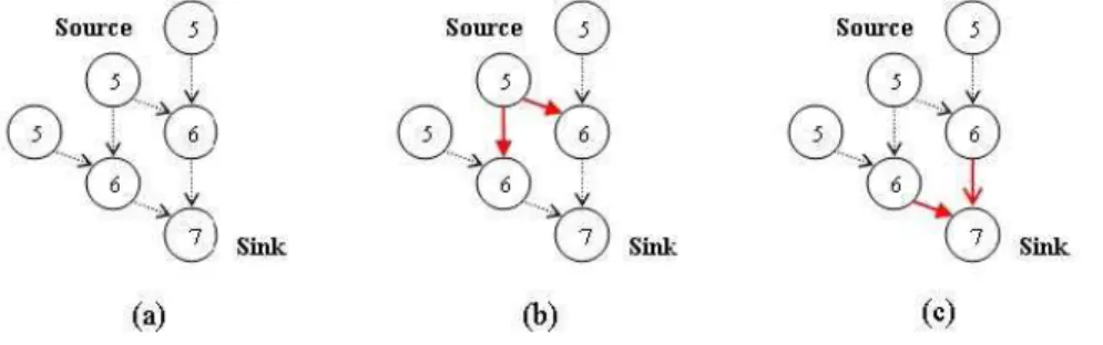
The task breakdown and project timeline is illustrated in Table 1. What highlighted are tasks completed so far. We have completed what have been planned for the first two years. In particular, for the service differentiation parts, we are ahead of the schedule.

Timeline Tasks Work

Flow Adaptive

Diffusion Fast Forwarding

Service

Differentiation Lit. Review Data-centric _delivery String search _algorithm Sensor network _QoS 1st Year Design Bandwidth usage and delay

analysis Protocol Specification Complexity analysis Pseudo code Data prioritization for desired QoS Mechanism

Evaluation ns-2-based _simulation

Implementation on Linux-based embedded systems ns-2-based simulation 2nd Year Validation Implementation and APIs on sensor notes Implementation and APIs on sensor nodes Implementation and APIs on networked embedded Linux devices 3rd Year Deployment Integration and porting of the adaptive diffusion, fast forwarding, and service differentiation mechanisms to the actual devices

三、成果自評與展望

On results of magnetic diffusion [1] for data-centric routing is published in a selective international conference with the acceptance rate is 21.8%, the 8th ACM/IEEE

International Symposium on Modeling, Analysis and Simulation of Wireless and Mobile Systems (MSWiM 2005). Subsequently, we submit the enhanced version [2] with more detailed results to Computer Communication (SCI) and the journal version is published August 2006. Our work on fast forwarding algorithm comparison is completed. The design, experimental results, and discussion are detailed in a master thesis [3]. A shorter version of the thesis is also submitted for publication [4]. Testbed establishment and evaluation on service differentiation for timely reliable data delivery is presented partly in [5] and detailed in a master thesis [6]. A concise version is under preparation for journal publication. The mechanisms and

evaluations are detailed in the subsequent 分析與討論 sections of this report. Other sensor network research on indoor localization has also received promising results. The idea of accelerometer-assisted energy-efficient location sampling technique is well received. An application of the idea on boundary detection [7] is published in IEEE PerCom 2006 and the extended version [8] is under revision to IEEE Transasction on Mobile Computing. Another application of the idea on our Zigbee-based indoor localization system [9] is published in IEEE SECON 2006. The extended version [10] of the work is invited and subsequently to appear in Ad Hoc Networks in 2008.

Our research activities have been noted by the international community. The project PI, Prof. Polly Huang, is invited to serve on the technical program committee of ACM SenSys 2007and HotEmNets 2008. ACM SenSys with a 10ish% is the flagship conference in the sensor network area and HotEmNets is the venue where the community shares the latest ideas.

On top of the research activities, our sensor network testbed, deployed in the Barry-Lam Hall of EECS NTU, is one of the largest and running testbed in Taiwan. The sensor networking mechanisms developed by this project and the indoor

localization work are integrated and working reliably on the testbed. The project PI has hosted more than 20 visits and 100 visitors from the industry, academia, NSC, as well as NSF representatives from the US. The demo videos are available at:

http://nslab.ee.ntu.edu.tw/demo/{BL-elevator.avi, BL-uhealth.wmv}

Looking forward to continue our work, we propose to investigate in depth the properties of data transmission over the physical sensor network testbed in office buildings. We observe in prior work that, even with routing and forwarding mechanisms designed for high quality of service (QoS), the delivery ratio of the sensor data varies depending on the (1) structure of the building, (2) building material, (3) human traffic, (4) the use of conflicting radio devices in the building, (5) weather, and (6) subtle differences in the sensor node hardware. These factors may impact the spatial and temporal stability of the sensor data delivery drastically. Given the advances in architectural and interior design, as well as very mobile and ubiquitous wireless communication lifestyle, we think that one of the key issues towards wide-spread use of sensor networks is the scalability and robustness of sensor

Knowing that the quality of sensor data delivery is not an issue that can be solved solely by a well-designed communication protocol suite, our aim in the follow-up project is to investigate in depth the environmental, protocol design, and

deployment factors to the quality of data dissemination in sensor networks. Our

premise is to develop, in a three year timeframe, a practical indoor sensor network deployment scheme, which may include a set of assistive software/hardware tools. The deployment scheme will enable easy deployment of quasi-reliable sensor networks in heterogeneous indoor environment. Our ultimate goal is to complete progressively a series of study towards effective sensor network deployment scheme for heterogeneous indoor environment: (1) to come to a fundamental understanding of the link quality distribution, (2) to perform a network- and MAC-layer protocol co-analysis, and (3) to design an effective sensor network deployment mechanism.

[1] Hsing-Jung Huang; Ting-Hao Chang; Shu-Yu Hu; Polly Huang, Magnetic

Diffusion: Disseminating Mission-Critical Data for Dynamic Sensor Networks, In the proceedings of the 8th ACM/IEEE International

Symposium on Modeling, Analysis and Simulation of Wireless and Mobile Systems (MSWiM 2005), Montreal, Qc. Canada, October 10-13, 2005

[2] Hsing-Jung Huang; Ting-Hao Chang; Shu-Yu Hu; Polly Huang, Magnetic

Diffusion: Scalability, Reliability, and QoS of Data Dissemination Mechanisms for Wireless Sensor Networks, Computer Communications,

Vol. 29, No. 13,, pp. 2482-2493, Aug. 2006

[3] Jui-Chieh Wu, Suffix Tree for Fast Sensor Data Forwarding, Master Thesis, National Taiwan University, June 2006.

[4] Jui-Chieh Wu, Hsueh-I Lu, Polly Huang, Suffix Tree for Fast Sensor Data

Forwarding, Under submission.

[5] Seng-Yong Lau, Ting-Hao Chang, Shu-Yu Hu, Hsing-Jung Huang, Lung-de Shyu, Chui-Ming Chiu, Polly Huang, “Sensor Networks for Everyday Use:

The BL-Live Experience,” IEEE International Conference on Sensor

Networks, Ubiquitous, and Trustworthy Computing (SUTC 2006), Industrial

Program, Taichung Taiwan, Jun. 2006.

[6] Ting-Hao Chang, Reliable Data Dissemination in Practical Sensor

Networks, Master Thesis, National Taiwan University, June 2006.

[7] Tsung-Han Lin, Polly Huang, Hao-Hua Chu, Hsing-Hau Chen, Ju-Peng Chen, Enabling Energy-Efficient and Quality Localization Services, In

the proceedings of the 4th IEEE International Conference on Pervasive Computing and Communications (PerCom 2006), Work in Progress Session,

Pisa Italy, March 2006

[8] Tsung-Han Lin, Chuang-Wen Yu, Polly Huang, Hao-hua Chu, Energy-efficient Boundary Detection for RF-Based Localization

Systems, In revision to IEEE Transaction on Mobile Computing (November

2006 submitted, September 2007 revision requested, December 2007 revision submitted)

[9] Chuang-wen You, Yi-Chao Chen, Hao-hua Chu, Polly Huang, Ji-Rung Chiang, Seng-Yong Lau, Sensor-Enhanced Mobility Prediction for

Energy-Efficient Localization, In the proceedings of the 3rd Annual IEEE Communications Society Conference on Sensor, Mesh and Ad Hoc

Communications and Networks (SECON 2006), Reston VA, USA,

[10] Chuang-wen You, Polly Huang, Hao-hua Chu, Yi-Chao Chen, Ji-Rung Chiang, Seng-Yong Lau, Impact of Sensor-Enhanced Mobility Prediction

for Energy-Efficient Localization, Elsevier Ad Hoc Networks, Invited

四、分析與討論之一 — Magnetic Diffusion for Disseminating Mission-Critical Data for Sensor Networks

4.1. Introduction

The technological advances have enlightened a future of intelligent and pervasive computing and communication. In that, miniature and robust sensor nodes would be able to generate, pre-process, and communicate metrics about the environment. For instance, auto-sensing of the room temperature allows tuning of the air conditioning to the level just as necessary. Auto-detection of pulse anomalies allows prevention of irreversible damages caused by diseases that are preceded by arrhythmia.

Envisioning a new generation of sensor network applications in healthcare , we seek mechanisms that provide reliable and timely transmissions of mission-critical data. the sensor nodes are likely to run on limited battery power for the ease of deployment. Thus, energy efficiency remains an important design challenge. Much of the related work in sensor network data dissemination either emphasizes on the energy efficient design or the reliable data transfer. We have not yet been able to identify any

mechanism comparable to the proposed mechanism, magnetic diffusion (MD) that aims at achieving timely delivery, reliability, and energy efficiency.

MD is a simple data dissemination mechanism that promises all the above properties. The inspiration comes from the magnetic interactions in the nature. Consider the data sink as a magnet and the data as nails. The data will be attracted towards the sink according to the magnetic field just as the metallic nails being attracted towards the magnet. The magnetic field is established by setting up the proper magnetic charges on the sensor nodes within the range of data sink. The strength of the charge is determined by the hop distance to the sink and the level of resource available at the sink. The data will be propagated based on the magnetic field from low to high magnetically charged nodes. This way of disseminating data results in optimal delay multi-path forwarding.

We are able to observe from the simulation results that MD does 1) perform the best in timely delivery of data, 2) achieve high data reliability in the presence of network dynamics, and yet 3) work as energy efficiently as the state of the art mechanisms. We thus conclude that MD is a promising data dissemination solution to the mission-critical applications such as home care and telemedicine.

There is a significant volume of related work in sensor network data dissemination. MD is particularly related to research in energy efficient routing and reliable data delivery. To put our work in context, we compare and contrast the existing work to our mechanism. In general, we are not able to identify any mechanisms comparable to MD that aims at achieving timely delivery, reliability, and energy efficiency. This is primarily due to the limited attention in sensor network design for mission-critical applications.

We choose to compare MD to the mechanisms that we are able to finnd actual implementations for the frequently-used Motes/TinyOS platform [28][29]. Directed diffusion [30][31] and flooding are the mechanisms considered in our evaluation. To facilitate discussions in the later sections, we give an overview of the directed diffusion mechanism, following the summary of existing work.

4.2.1 Energy efficient data dissemination

There are three major classes of energy efficient data dissemination mechanisms, the cluster-based, random-walk, and location-aware mechanisms. The cluster-based approaches [3] [32] [33] evenly distribute energy load among the sensors in the network. The idea is to form clusters for localized data dissemination and send only the aggregated data across the clusters to conserve energy. Random-walk approaches [26] [34] randomly select the next hop targets to disseminate data. These mechanisms are energy efficient in that they avoid the sending of control messages and the

maintenance of routing states. Location-aware schemes [35][36] exploit the nodes' geographical location information to minimize the cost of disseminating data. The location information might not be easy to obtain for certain sensor network

applications. More closely related to our work are the mechanisms dealing with efficient data dissemination to mobile sinks [37][38]. MD is similar in that our mechanism also aims at energy efficient data dissemination for dynamic networks. MD is yet different for that the mechanism design takes into account mobile non-sink nodes and considers the on-off type of network dynamics.

4.2.2 Reliable data dissemination

There are two major approaches towards better data delivery reliability. The passive approach retransmits data when losses are detected, whereas the active approach aims, instead, at avoiding losses. More specifically in the passive approach category, some proposed mechanisms [39][40] recover data end-to-end, and the others [41][42] retransmit hop-by-hop. In the end-to-end mechanisms, the sink nodes track the status of data delivery and send request messages to other nodes for recovery.

The hop-by-hop mechanisms implement the data recovery between two neighboring nodes. When a data packet is lost, the intermediate sending node retransmits. In the active approach category, several schemes [43][44][45] attempt to improve reliability by avoiding congestions. By avoiding congestions, these schemes indirectly lower the loss rate and improve the overall reliability. In addition, some schemes [46][47][48] avoid losses by selecting less lossy data paths.

Our work is closely related to [49], a multi-path mechanism. This work has suggested that disseminating data over multiple paths improves the reliability. The number of paths selected in the mechanism depends on the priority of the data and the network situation. Our MD is similar to this mechanism in that we also disseminate data over multiple paths for reliability. The primary difference is in our choices of the multiple paths. Opting for energy efficiency and timeliness of data delivery, we scope our choice to all the available shortest paths.

4.2.3 Directed Diffusion

Directed diffusion [1][2] is a data-centric data dissemination protocol for wireless sensor networks. The mechanism achieves energy efficiency by means of selecting empirically good paths and in-network aggregation. There are two dissemination modes in directed diffusion: one-phase pull and two-phase pull.

One-Phase Pull (OPP). In OPP, the sink periodically broadcasts an interest

message to each of its neighbors. The interest message specifies the data the sink is interested. The neighboring nodes continue to broadcast the interest message to their own neighbors if the interest message is not a duplicate. This action will be repeated until all nodes have received the interest message. Then, the source with the matching data selects the path of shortest latency according to the interest arrival time, and disseminates data to the sink. The data path is periodically refreshed by interest messages.

Two-Phase Pull (TPP). TPP operates in a similar way with a slight

complication. The sink also periodically broadcasts an interest message to its

neighbors, and the neighbors operate similarly to those in OPP. The main difference is at the broadcasting of exploratory data from the data source to all nodes in the sensor network. After the sink receives this exploratory data packet, it reinforces a good path back upstream by sending a reinforcement message. This reinforced path is

determined according to metrics such as delay, loss rate, and available bandwidth. The node that receives the reinforcement message acts in the same way and forwards the reinforcement message back upstream until the source receives this reinforcement message. After that, the source sends data along the reinforced path.

To adapt to network dynamics, the reinforced path is periodically refreshed by

periodic exploratory data. To conserve energy due to the flooding of data packets, the interval of periodic exploratory data is set to be significantly longer than that of the periodic interest messages. Please note following important differences between OPP and TPP that will be referred later while comparing the performance of OPP, TPP and MD:

A. To avoid collisions, TPP implements its own random wait mechanism to prevent synchronized sending of exploratory data. Each node selects a random waiting time when receiving an exploratory data. There is only one data transmission path in OPP. It does not need to schedule a random wait before propagating data.

B. To adapt to failures, OPP refreshes the data path by periodic interest message, whereas TPP refreshes the reinforced path by periodic exploratory data. C. The frequencies of sending exploratory data and interest messages are

different. The frequency of periodic exploratory data is twice as low as that of periodic interest messages.

4. 3. MAGNETIC DIFFUSION

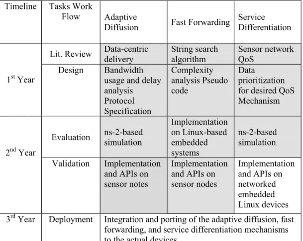
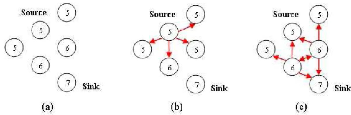
Magnetic diffusion is simple and yet powerful. Consider the data sink as a magnet and the data as metallic nails. The data will be attracted towards the sink according to the magnetic field just as the nails are attracted towards the magnet. The magnetic field is established by setting up the proper magnetic charges on the sensor nodes within the magnetic influence of the data sink. The strength of the charge is determined by both the hop distance to the sink and the level of resource available on the sink. The data will be propagated based on the magnetic field from low-charge to high-charge nodes (Figure 2-a). This way of disseminating data promises the following properties.

Multiple Paths. By the simple principle of data traveling towards the center of

attraction, the sensor nodes forward data coming strictly from the nodes with lower charges (Figure 2-b). Forwarding data this way, the paths selected by MD are optimal. Furthermore, there can be multiple next hops to forward the data. Thus, MD sends data in an optimal multi-path fashion.

Load Balancing. When there are multiple magnets in the environment, the

multiple magnetic fields will find their balance. The nails will thus be attracted by the magnets nearby. The same principle applies to MD. When there exist multiple sinks, their magnetic influences, decrementing MD charges from the sinks, will strike a balance (Figure 2-c) and attracts the data nearby. One advantage of such property is that whenever a new sink joins or an old sink leaves this system, a new balance will

be re-established automatically.

Resource Awareness. In the real world, some data sinks might be more

resource-limited than the others. For example, there could be sink nodes supplied by unlimited wall-power, while others run on batteries. By assigning sink charges based on the amount of resource at hand, we can achieve the goal of balancing the use of heterogeneous re- source and potentially prolonging the network lifetime without human intervention.

Figure 2-a. Data move toward magnet (i.e. sink).

Figure 2-b. Multiple paths: multiple nodes with equal charge, s1 < s2 < s3.

Figure 2-c. Load Balancing: multiple magnets attracting nearby nails. Figure 2. Illustration of Magnetic Diffusion

In a healthcare example, a patient with chronic diseases may wear biometric sensors for long-term monitoring of the patient's body temperature, blood pressure, and heart rate. These sensor data need to be collected to a remote patient record server for further analysis. When the patient goes outdoors where there are no infrastructural sinks, the sensor data need to be transmitted to a resource-limited personal device such as the patient's PDA. Through a GPRS interface, the sensor data can be transmitted to the patient record server. When the patient comes back home, or

wherever there are more resourceful sinks such as a full edged PC with low-cost ADSL connection, one can assign a stronger magnetic charge to the PC. Then the data, aware of the stronger attraction, will go through the PC rather than the PDA(Figure 3). Such resource-aware feature brings not only convenience but also optimized

utilization of the resources in the environment.

Figure 3-a. Small magnet (resource limited sink, ex:PDA) attract data and transmit via resource limited network (ex:GPRS) to Internet.

Figure 3-b. Large magnet (more resourceful sink, ex:PC) which overwhelm small magnet, attract data and transmit via wider bandwidth network (ex:ADSL) to Internet Figure 3. Resource-awareness: larger magnet out-attracting the small magnet

MD operates in two phases: the interest broadcast and data propagation. The magnetic field is established in the interest broadcast phase such that the data can be

disseminated towards the sink in the data propagation phase. In the subsections below, we describe the details of the MD operation and the implementation options.

4.3.1 Interest Broadcast

We first introduce two data entities involved in the interest broadcast phase: the interest and the entry. The interest is a message used to establish the magnetic field to facilitate the proper flow of data toward the sink. An interest message consists of two elements, the data type and magnetic charge. The former records what data type the sink wants to collect. The latter is an integer value recording the strength of the magnetic influence from the sink. The entry is where a node records the data type and the magnetic charge in each node.

When a sink wants to collect data, it sends an interest message to its neighbors. When a node receives an interest message for the first time, it creates an entry for this interest. Then the node decrement the magnetic charge in the interest by one. The

node records the data type and the magnetic charge into its entry and then forwards the interest message to its neighbors. The decrementing magnetic charges from the sink to source will guide the flow of data in the reverse direction, mimicing the traveral of metallic nails from the low-charge to high-charge points in the magnetic field.

If a node receives an interest message and the corresponding entry exists, it will compare the decremented magnetic charge of the interest with the one in the entry. If the magnetic charge of the interest is greater than the one in the entry, the node will update the value in the entry to that of the interest and forward the interests to its neighbors. Otherwise, the node will discard the interest knowing the interest is not from a node closer to the current sink. The sink node will broadcast interest messages periodically to re-establish proper magnetic charges in case of network dynamics. It provides a robust environment especially for the dynamic network.

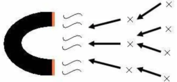
In Figure 4(a), the sink node broadcasts the interest to its neighbor nodes. In Figure 4(b), both nodes, A and B receive the interest, create corresponding entries, set the data type and proper magnetic charges in the entries, and then propagate the interests to their neighbors. In Figure 4(c), node C, D, and E receive the interests from node A and B and repeat the actions taken by A and B in Figure 4(b). Each node may receive and discard duplicate interests or interests of weaker magnetic charges.

Figure 4. An example of interest propagation.

4.3.2 Data Propagation

We next describe how the data is disseminated through a network. We have two implementation strategies for data propagation. One is gradient-based and the other is broadcast based.

4.3.2.1 Gradient-based

nodes with a stronger magnetic charge, the node will establish a gradient toward the interest-sending node. This gradient will lead the data through the network from the source to the sink.

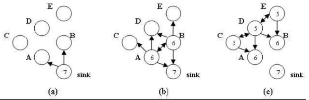
When a node senses data, it checks if it has an entry matching the data type. If it does, the node sends the data to the nodes pointed by the existing gradients. The receiving nodes check for the matching entry and then send the data according to the gradients as well. The forwarding process goes on and the data will reach the sink eventually. Figure 5(a) shows the gradients established by the interest broadcast in Figure 4. In Figure 5(b), the source sends data to the two neighbor nodes pointed by the gradients from the source. In Figure 5(c), the receiving nodes continue to send data to their neighbor nodes based on their gradients. The sink finally receives the data.

Figure 5. An example of data propagation with gradient-based mechanism.

4.3.2.2 Broadcast-based

In the broadcast-based mode, the nodes do not establish gradients in the interest broadcast phase. Instead, the magnetic charge is included in the data being

disseminated. The receiving node can tell from the charge carried in the data where the data is coming from and whether to forward the data further down the stream. More specifically, when a node receives the data, the node checks if it has any matching entry. If so, it compares the magnetic charge in the entry with the magnetic charge of the data. If the magnetic charge in the entry is greater than that of the data, it sets the magnetic charge of the data to the charge in the entry and then broadcasts the data. This means the data is sent from the node whose magnetic charge is lower than the intermediate node and the intermediate node should continue to broadcast them toward the sink. If a node receives a duplicate data or the data whose magnetic charge is greater than or equal to that in the entry, the data will be discarded.

gradients. The node simply compares the magnetic charges to decide whether to broadcast the data. The drawback is every data message will have to carry the magnetic charge of the sending node.

Figure 6. An example of data propagation with broadcast-based mechanism.

In Figure 6(a), the magnetic charge of every node is established with the sink having change strength 7. In Figure 6(b), when the source wants to send data to the sink, it will broadcast the data to its neighbor nodes. In Figure 6(c), the nodes with charge strength 6 broadcast the data because the magnetic charge of the nodes is greater than that of the data. Thus, the sink receives the data.

4.3.3 Random Wait

When the interests or data are being broadcast hop by hop through the network, the messages might collide to each other. To avoid collisions, the node waits a random period of time before sending a message. This technique might decrease the

probability of collision and, in the meantime, increase the transmission delay.

4.4. EVALUATION

We have conducted an extensive set of simulations that examines the scalability of MD to the size of the network, the change of the data rate, and the level of the network dynamics. In this evaluation, we are particularly interested in the performance of MD in dynamic networks. Thus, we focus our discussion on the quality of data delivery and the message overhead of MD in the presence of network dynamics.

Nodes 50

Size 160 x 160

Radio range 40 m

Data rate 5 sec

Periodic Interest 30 sec

Antenna OmniAntenna Simulation time 600 sec

Table 2. Simulation setup

4.4.1 Simulation Setup and Metrics

In this section, we describe the simulation setup and the metrics examined for the performance evaluation. We implemented MD in the ns-2 simulator [50]. In order to get the average behavior, there are 10 distinct runs for each setup. In each run, there are 50 nodes randomly placed in a 160m by 160m square. Each node has a radio range of 40m. We use one source and one sink randomly selected from 50 nodes in our simulation. The source sends data every 5 seconds, and the interests are

periodically sent every 30 seconds. The simulation time is 600 seconds, but source will stop sending data after 300 seconds. Table 2 summarizes the parameters of our choice.

We choose three metrics to evaluate the performance of MD and to compare it to other schemes: Overhead measures the amount of interest and data packets

transmitted. The metric is closely related to the energy consumption of the system in wireless sensor networks when an energy efficient MAC protocol is applied.

Reachability measures the probability the sink receives the data packet successfully.

This metric is important for medical applications in that the sensor data are mission critical and data losses can be life-or-death matters. Latency measures the data transmission time from the source to the sink. For medical applications, the metric represents the timeliness and temporal reliability of the data.

The MD implementation used in our experiments is the broadcast mode. There are several advantages of the MD broadcast (MDB) mode over the gradient (MDG) mode. MDB is more energy efficient. The interest packet overhead of the two modes are the same because interests are transmitted in an identical way in both modes. The

difference lies in the data packet overhead. In MDG, if a node has five gradients to its neighbors, there are five packets sent, one for each gradient. But in MDB, it

broadcasts only one data packet. Therefore, the overall overhead of MDB is much smaller than MDG. Additionally, the data latency is small in MDB. It does not need to send the handshake packets, e.g., the RTS/CTS in IEEE 802.11, before sending a data packet, but MDG does. As a result, MDB behaves better in latency. However, without the handshaking, there are more collisions observed in MDB simulations, and this results in a slight lower reachability in some cases. MDB performs also better in the presence of network dynamics. Given the various advantages of the MDB over MDG,

we use MDB for the rest of the comparison.

4.4.2 Impact of Dynamics

To be realistic, we simulated two kinds of dynamics in our experiments. First of all, we simulated mobile environment in which nodes moved around every 120 seconds. It means that the first movement of each node occurs at 120 seconds. After a node moves to its new position, it waits another 120 seconds to move again. The amount of time that a node takes to move to its new position varies from node to node because of the random new position selection. As a result, the movement of the nodes are not simultaneous.

Second of all, we simulated random node on and off according to the following probabilistic distribution. At the beginning, all nodes are in the on state for a random period between 5 to 65 seconds. Then each node goes into the off state for 25 to 35 seconds, and wake up again for 55 to 65 seconds. All the on or off time durations are uniform randomly selected. and this process will continue until the end of the

simulations. These sets of simulations are necessary because the two dynamics are common in reality. The choices of the parameters represent the extreme cases to highlight the distinct properties in MD to the other two mechanisms, DD (See Section 4.2.3.) and flooding, compared.

4.4.2.1 Overhead

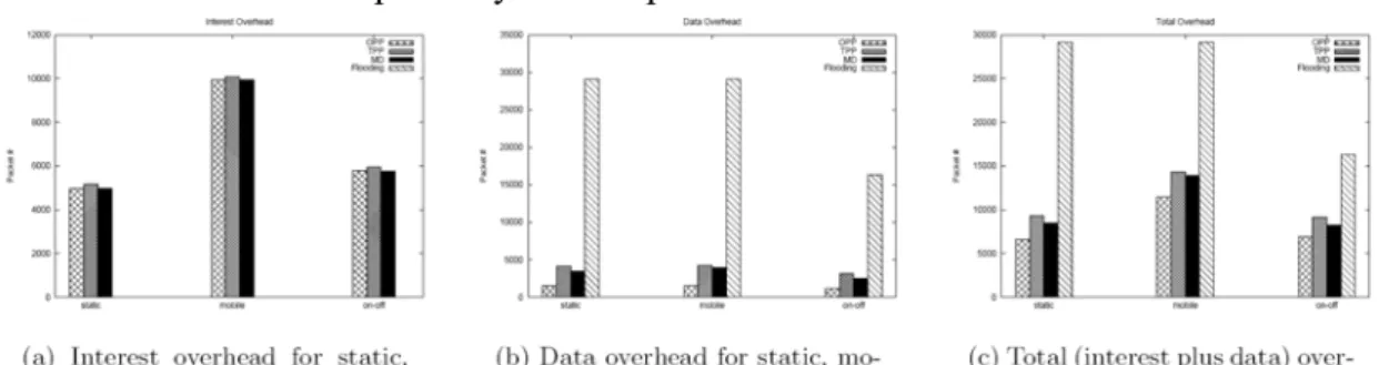
Figure 7 shows the amount of overhead for the static, mobile, and on-off cases. Note that in the static case, all nodes remain static and on for the entire duration of the simulations. We show the static case result here to compare to the mobile and on-off cases. In Figure 7(a), the interest packet overhead of TPP is slightly higher than that of OPP and MD in all cases. This is because TPP has to disseminate additional control packets such as the positive and negative reinforcement messages, whereas MD and OPP do not. Note that we set the interval of periodic interest to 30 seconds in all mechanisms. That is the reason that the interest packet overhead of MD and OPP are almost identical.

Figure 7(b) shows that MD has a lower data packet overhead than that of the TPP and a higher data overhead over that of the OPP in all cases. OPP selects only one way to disseminate data, and thus has the least amount of data packet overhead. This result suggests that, independent of the static, mobile, or on-off case, the resulting data packet overhead of TPP's exploratory data is higher than that of the multi-path delivery in MD, and that MD is more energy efficient than TPP. It seems that MD is worse than OPP in terms of data packet overhead. However, the higher data overhead,

in return, provides better data reachability and latency which will be discussed next. Figure 7(c) shows that flooding has the largest total packet overhead even though the mechanism does not require any control packets.

Figure 7. Overhead.

4.4.2.2 Reachability

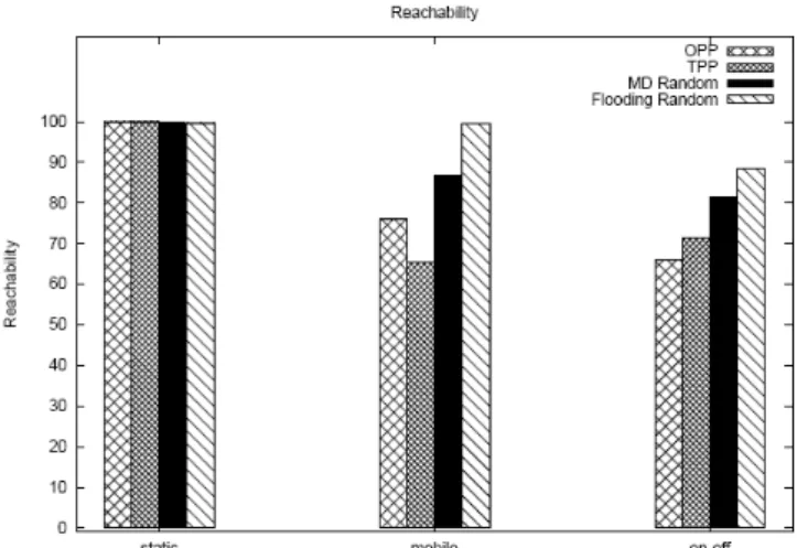
Figure 8 shows the reachability results of the static, mobile, and on-off cases. In the static case, OPP and TPP experience an 100% reachability, MD and flooding's reachability is at about 98%. The reason of the difference is at the way the data are propagated. OPP and TPP are gradient-based, whereas MD and flooding are broadcast-based. If data packets collide, the gradient-based mechanisms will retransmit assuming IEEE 802.11 as the underlying MAC protocol. The

broadcast-based mechanisms, however, do not detect, nor recover for errors, and thus the slightly lower reachability observed in MD and flooding.

Figure 8. Reachability for static, mobile, and on-off case

In the mobile case, the reachabilities of OPP and TPP drop significantly. MD's reachability is reduced to 85%, which is about 20% higher than TPP (65%) and 10% higher than OPP (75%). This is because MD sends data in multiple paths. When the nodes are mobile, the probability is higher to get the data through the network to the sink with multiple paths.

Note that TPP performs worse than OPP in the mobile case. The difference lies in the path update frequency. OPP reconfigures data path at the time of periodic interest, but TPP does so at the time of periodic exploratory data. The interval of periodic

exploratory data is twice as much as the periodic interest. Therefore, TPP results in a lowest reachability in this case. If we shortened the time of periodic exploratory data, there will be a higher reachability, but the data packet overhead will also increase. From this set of results, we can see the advantages of MD over OPP and TPP in terms of reachability in mobile sensor networks. Note that the reachability of flooding is close to 100%. The result suggests that if the data is absolutely critical and energy is not a constraint, flooding is the best choice for reliable data dissemination. Otherwise, MD provides as a reliable solution for environment that energy resource is limited. In the on-off case, we observe similar results. But the performance is unsatisfactory., Even the flooding mechanism manages only an 85% reachability. This is because of the potential of broken paths, or even a disconnected network, when certain

bottleneck nodes are turned off. Such conditions result in a lower overall reachability. However, we think that a good deployment strategy may compensate for such

situations.

We find that OPP performs the worst in the on-off case. In some sense, the on-off type dynamic presents greater challenge to reliable delivery of data and OPP, or single-path mechanisms, is less suitable for networks with extreme dynamics.

4.4.2.3 Latency

Figure 9 shows the cumulative probability of data delivery latency for the static, mobile, and on-off cases. In Figure 9(a), MD has the least latency because it broadcasts data and bypasses the RTS/CST handshake in IEEE 802.11. This is also why OPP performs much worse than MD, even if it always finds the fastest path. Flooding is better than OPP and TPP only in the preceding 60%. We observe an unusual amount of traffic and collisions in the flooding set of simulations, As a result, some data packets get retransmitted repeatedly and routed for a long way to finally reach the sink. This explains why flooding has a lot of data packets with long latency. TPP is very close to OPP in the preceding 90%, but there is a long tail caused by the random wait mechanism in disseminating exploratory data in the later 10%. This plot shows that the broadcast-based mechanisms work better for applications with latency requirements.

In Figure 9(b), MD has the least latency yet. Note that Flooding performs better than OPP completely. This is because OPP has to retransmit a packet many times as a result of high frequency of packet loss and collision in mobile networks. The same reason in OPP and lost data packets result in the poor performance of TPP. Figure 9(c) shows similar result as well. These results indicate that MD is a better solution for applications with requirements of restricted latency in dynamic network.

Figure9. Latency.

4.4.3 Impact of Random Wait

Figure 10 shows the reachability after adding random wait mechanism to MD and flooding. The figure clearly shows that MD and flooding are improved significantly in all static, mobile, and on-o_ cases. In the static case, MD and flooding are better than the previous result (Figure 8) and the reachabilities are close to 100%. In the mobile case, MD and flooding maintain the same level of reachability. In the on-off scenario, however, advances on MD and flooding can be clearly identified. These results show that random wait mechanism is effective in reducing collisions and thus improve reachability.

Figure 11(a) shows cumulative distribution of delay for static environment. Contrary to the previous result, MD performs slightly worse than OPP and TPP here. This is because the random wait mechanism incurs a longer data delivery latency. It does not have the long tail as in TPP though. As expected, the curve of flooding shifts to the right as what happened to MD. Figure 11(b) shows also the trend that the curves of MD and flooding shift to the right. But MD performs as well as OPP. TPP is the worst in latency. Figure 11(c) shows similar results to Figure 11(a) except the overall

amount of data received in MD and flooding simulations is higher.

These results show a trade-off between reachability and latency. The cost of a higher reachability is often the longer latency. One may trade-off a little reachability for much shorter latency. Whether to implement random wait depends on the

random wait will be a good option. If the latency is more critical, it is more appropriate to turn off the random wait mechanism.

Figure 10. Reachability for static, mobile, and on-off case after adding random wait to MD and Flooding

Figure 11. Latency.

4.5. CONCLUSION

Inspired by the physics of magnets and nails, we propose magnetic diffusion, a simple and yet efficient dissemination mechanism for mission-critical data. MD is able to identify all the shortest paths available from the data source to sink. By transmitting data over the multiple shortest paths, MD performs well in the timeliness and

reliability of data delivery while the overhead and energy consumption of MD is kept low. These properties are confirmed by the simulations. Therefore, we conclude that MD is particularly suitable for sensor network applications in healthcare and

workplace safety. For these applications, the timeliness and reliability of data, and the energy efficiency of the system are all required properties.

五、分析與討論之二 — Fast Forwarding: Suffix Trees for Fast Sensor Data

5.1. INTRODUCTION

On the address-centric Internet, communication nodes are numerically addressed, for example, 140.112.42.220. A source node sends data by the destination node’s address. Forwarding, also known as the routing table lookup problem, involves how, given the destination address of an incoming data packet, each intermediate router locates a matching entry in the routing table. From the matching entry, the router identifies the network interfaces (or ports) towards the next hops that the data packet should be forwarded further. Efficient algorithms and data structures such as [50] are proposed to speed up the number matching, which lead to the design of very high-speed IP switches today. Motivated to achieve high-speed forwarding for sensor networks, we seek efficient algorithms and data structures to speed up string matching for

data-centric sensor networks.

In data-centric wireless sensor networks [51], nodes are no longer addressed. Data do not carry the destination address. Instead, each sink node sends an explicit interest through the network to draw in a particular type of data. The intermediate nodes in turn disseminate the data based on the data content rather than the destination node’s address. This data-centric style of communication is particularly promising for that it alleviates the effort of node addressing and address reconfiguration in large-scale mobile sensor networks.

Figure. 12. An example of interest matching.

Forwarding in data-centric sensor networks is particularly challenging. It involves matching of the data content, i.e., string-based attributes and values, instead of numeric addresses. This content-based forwarding problem is well studied in the domain of publish-subscribe systems. It is estimated in [52] that the time it takes to

match an incoming data to a particular interest ranges from 10s to 100s milliseconds. This processing delay is several orders of magnitudes higher than the propagation and transmission delay.

Consider the MicaZ [53] and TinyOS [54] sensor network development platform. The packet size limit is 36 bytes. The wireless radio transmits at 100s kbps. The

transmission delay is thus at the scale of 1s milliseconds. Assume 10 meter radio range and 2x108m/s propagation speed The propagation delay can be found at the scale of 0.01s microseconds. The processing delay is evidently the bottleneck of the per hop forwarding delay. The interest lookup delay is contributed by 2 levels of matching - interest and predicate matching. Each interest may consist of multiple predicates. At the higher level, the system needs to identify, among various interests, a particular interest that matches the incoming data. At the lower level, the system verifies whether a predicate in an interest matches the incoming data. Illustrated in Figure 12 are 3 example interests composed by a number of predicates. Interest 1 is looking for anything related to the nslab group. Interest 2 looks for data about a faculty member whose name is polly, and interest 3 looks for data about all 2nd year and above master students. The incoming data in Figure 12 matches both interests 1 and 2.

Much of the recent work [55][56][57][58] focus on the strategies of structuring interests or content types to enable fast interest matching. Their objective is to reduce the number of predicate matching required. Our work complements these earlier studies in that we focus on improving the efficiency of individual predicate matching. Predicate matching involves attribute matching and value matching. Attribute

matching is essentially an exact string matching problem. One common practice to speed up attribute matching is to fix the bit position of all possible attributes in the data packet as well as the routing table. This method, although simplifies the attribute matching process, will be memory and bandwidth consuming when the number of different data types is high. When there are different sensors to be added to the network, the system will not be easily extendable without changing the packet format and interest table data structure. Value matching is also a string matching problem, when the data type is string. Depending on the operator of the predicate, value matching may require exact or sub-string matching. In essence, the efficiency of predicate is determined by the efficiency of the string matching algorithm used. For efficient string matching, prior work [7] suggests the use of ternary search tree (TST). It is a string matching algorithm with O(|P|+log(N)) time complexity and O(|S|)

space complexity. P denotes the input string, typically an attribute or value string in the incoming data. S denotes the training word set which concatenates all the strings appear in the entire interest table. N denotes the total number of strings in the training set. To speed up the string matching process further, we propose and evaluate the use of suffix tree (ST), a linear time string matching algorithm that can be easily extended to perform efficient prefix, suffix and substring matching. ST has an O(|P|) time and O(|S|) space complexity [59][60].

Although the large-scale performance of TST and ST’s memory requirement is the same, we find, in real implementations, the amount of memory required by ST is significantly higher than that of TST. This is a serious problem for sensor nodes in which the memory space is very limited. To tackle the problem, we further propose a scheme to optimize the memory consumption for ST.

To observe how the algorithms will perform in practice, we implement TST and ST, as well as a simple hash-based method for comparison. The experimental results show that the computation time is reduced by 29% to confirm a match and 48% to confirm a non-match at best. The memory usage of ST is improved by 24% with the memory optimization scheme.

Our contribution is three-fold: (1) we identify ST for scalable sensor data forwarding, (2) we propose a novel optimization for ST to reduce the space requirement, and (3) we implement four string matching algorithms and evaluate how well they will perform in practice. The remainder of this thesis is organized as follows. The related work is presented next in Section 5.2. We describe then in Section 5.3 the string matching algorithms. Next in Section 5.4, we provide an analytical comparison of the algorithms. In Sections 5.5, 5.6, and 5.7 we detail the experimental setup, results, and our findings on how the algorithms perform in practice.

5.2. RELATED WORK

5.2.1. Data-Centric Communication

In the traditional IP network, nodes communicate to each other by the fixed IP addresses. This communication model is proven, by the daily operation of Internet, effective in supporting applications running on static and full-fledged computers. For mobile and resource-limited sensor networks, how to configure and reconfigure node addresses in the presence of node dynamics poses a great challenge. This problem is first raised and addressed in one of the pioneer work on sensor networks [51]. In that, the authors propose the data-centric communication paradigm.

In data-centric communication, digital information are disseminated based on the feature/attribute/content of the information itself, not the addresses of issuers or receivers. In the first data-centric routing mechanism for wireless sensor networks [1], sinks send explicit interest packets to set up routing states at the intermediate nodes. These interest specific routing states in turn draw in the data of interest for the sinks. Such dissemination scheme relies on well-defined naming system to describe data attributes and sink interests. The corresponding naming system and the filter-based forwarding mechanism are detailed in [55]. The string matching problem, although recognized as the performance bottleneck, is not addressed.

5.2.2. Publish/Subscribe Systems

In [7][61], the authors design a set of efficient forwarding and routing mechanisms for content-based data dissemination. The notion of content-based communication is essentially the same as data-centric communication. The mechanisms proposed, although descends from the literature of publish/subscribe systems, are applicable to sensor networks. There are two different kinds of publish/subscribe systems:

channel-based and content-based. In both systems, multiple users may subscribe to the data of interest. In channel-based systems, the users subscribe to a particular channel and the corresponding data broker pushes particular data to the channel from which the subscribing users receive the data. In content-based systems, the concept of channel is refined as rules and interests, traveling through the intermediate nodes between brokers and subscribers. If the rules belonging to some subscribers are matched by certain data, the data will be forwarded further to the indicated output ports, otherwise the data will be dropped by the node. Much of the improvement in rule matching concentrates on the management of the subscriptions, i.e., organization of predicates and rules. For instance, index algorithms, used also extensively in database management, are adopted by [56] to manage the subscriptions and speed up the matching process.

Other data structures such as button-up selection trees and binary decision diagrams are proposed to improve the matching performance by [57] and [58] respectively. Little work has addressed formally the problem of string matching.

5.2.3. Ad Hoc Publish/Subscribe Systems

The close relationship between publish/subscribe systems and data-centric sensor networks is first formally noted by [62]. The limited energy, computing power, and memory space on a typical wireless sensor node give rise to unique challenges in the design of data forwarding algorithms. Authors of [63] found that the interest diffusion mechanisms used by general publish/subscribe systems will not be suitable for

resource-limited wireless sensor networks. Energy-efficient routing schemes such as [64][65] are proposed to minimize the interest dissemination overhead. Despite the level of activities in energy-efficient publish-subscribe routing for sensor networks, the problem of efficient forwarding receives little attention.

5.2.4. String Matching Algorithms

String matching problems are well studied in the domain of bio-informatics, AI, and data mining. From the classic KMP [66] matching algorithm to the more recent ones, there has been a range of schemes proposed. TST [67] is a state-of- the-art algorithm that enables efficient binary search of strings. It is widely used in dictionary lookup and information retrieval.

ST [68] is a data structure for very high speed string matching. To handle dynamics in wireless sensor networks, an efficient algorithm must be able to insert attribute and value strings onto the suffix tree in an efficient ways. The online tree construction algorithm for suffix tree proposed by Ukkonen [59] satisfies the requirement. In [60], a memory improvement technique is presented to remove the redundancy inside internal nodes of suffix trees . Through the new data management of suffix tree, the space requirement of a static suffix tree can be reduced and be less than four integers per node in average. In this work, we adopt ST for string matching involved in the data forwarding process for sensor networks.

5.3. ALGORITHMS

We introduce in this section the four string matching algorithms in comparison. We begin with the straightforward algorithms, hash and TST. Details of the ST algorithm and its improvement will follow.

5.3.1. Hash

We use a rotation-based hash function [69] to construct the hash table of attribute and value strings and to search for strings in the hash table. The result of the hash function is calculated from the whole input string. Suppose every character in the string is coded as a number and s[i] represent the ith character in the string. For an n-character string, the hash value, h(n), is defined as follows:

h(n) = h(n − 1) << d + s[n − 1] h(0) = C

C is a pre-defined constant. We can obtain the hash value of an n-character string by iterating the shift and add operations n times. h(n) further takes a modulo m for a hash table of m slots. The final hash value is used to associate the string with the string’s

location in the hash table. A string with hash value j will be stored in the jth slot. Multiple strings might be hashed to the same slot. A simple linked list is used to handle the collisions. When a new interest packet is received, the attribute or value string will be inserted into the linked list at the corresponding slot. Similarly, when a data packet is received, the hash function is applied to obtain the hash values of the attribute and value strings. The system then may look up the hash table to see if there’s a matching attribute and value, i.e., a matching predicate.

5.3.2. Ternary Search Tree (TST )

String search using TST is similar to binary search. In TST, the data structure of a node contains a character and 4 pointers. The character is also known as the key for string comparison. Three of the pointers are used to track the decendant nodes cl, cm and cr, cl leads to substrings that begin with a character alphabatically smaller than the key. cm leads to substrings that begin with a character that equals the key.

Likewise, cr leads to substrings that begin with a character alphabatically greater than the key. When a match is identified, one follows the 4th pointer to the matched entry. Figure 13 shows the TST after inserting five words: egg, gas, get, aids, and bad. Following the principle of binary search, for an incoming string ”bad”, the search path on the tree will

be e → a → b → a → d.

The TST search algorithm is detailed below in Algorithm 1. To insert a string, one search on the existing TST first. From the branch the search stops, the remaining substring is attached to extend the TST. Let gdp be a string to be inserted into the TST in Figure 13, for example. The search stops at the g node on the right. To this end, part of the incoming string, g, is already be matched. To complete the insertion, new nodes representing the remaining substring, dp, will be created and attached one by one onto the branch.

Figure 13. An example of a ternary search tree.

5.3.3. Suffix Tree (ST )

The concept of suffix tree is better explained by a more intuitive data structure called

suffix trie. A suffix trie for a string S is a joint tree of its suffixes S1, S2, ..., to S|S|.

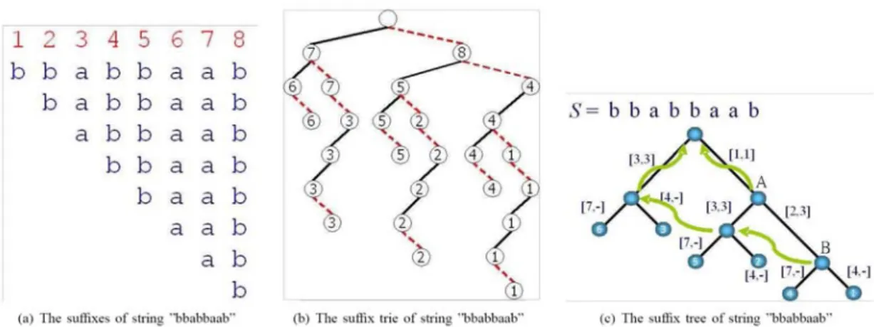
Let Si denotes the suffix of S starting from the ith character. For instance, in Figure 14(a), there are 8 suffixes for string bbabbaab, and bbaab is the forth suffix. Once we have the suffixes, we can build a suffix trie for the original string. Figure 14(b) shows the suffix trie of bbabbaab. The right (red dash) edge accounts for the character b and the left (black) one for a. The number on the leaves shows which suffix of the string on the interest table the incoming string matches to. Given the original string and the suffixes, it is trivial to extend the algorithm for substring matching. Any substring of bbabbaab must be the prefix of one of its suffixes. A naive method to create a

suffix trie is iteratively inserting the suffixes into the trie from the longest to the shortest. The construction cost is O(|S|2) steps, but it is clear that any substring search can finish in O(|P|) steps for any input string P.

ST retains this strong suit because it is essentially a compact representation of suffix trie. In a suffix trie, each edge carries one character. ST is more compact in that an edge on ST may carry a sequence of characters. A suffix trie can be transformed to an ST, and vice versa. Figure 14(c) is the ST of Figure 14(b). The pair-wise number on each edge denotes the beginning and end indices of the original string. For example [2,3] is to indicate the substring from the 2nd character to the 3rd, i.e., ba in the example. The numbers on the leaves represent the matched suffix. The curly (green) edges are traveled when none of the child matches. In this case, we can declare the exact match

fails.

As for the insertions, we adopt Ukkonen’s online construction [59]. With that, one can insert a new string T into ST by gradually adding characters T1, T2, ... , T|T| into the data structure without breaking any properties of the original tree.

Taking advantage of the suffix edges, each insertion can be completed in O(|T|) time. This fast construction of ST allows us to build a suffix tree in linear time. We apply ST on the attribute and value matching for sensor data forwarding. To enable exact string matching, each suffix tree is initialized by adding a special character $, which is considered a character that will never appear in any input strings. At the initialization stage, the ST, T , begins with an empty string followed by the special character, $. In each insertion, an input string Ti will be extended by adding one $ at its end and concatenates to the ST set, T . The string Ti$ is then added to the ST structure. After k insertion operations, the ST set, T , equals string $T1$T2$...$Tk−1$Tk$. An exact search for string P can be achieved by searching the string $P$ in T . Other string operations such as prefix and suffix can also be achieved by using strings like $P or P$ as input. We apply also a memory requirement reduction technique proposed in [60] to improve the scalability of ST in space.

Figure 14. Illustration of the relationship between suffix trie and tree

5.3.4. Suffix Tree with Space Improvement (ST+)

The drawback of ST is the high memory consumption. We conducted preliminary experiments to examine different possible sensor network related word sets on ST to check the space efficiency. The results shown in Figure 15 indicate that there are only 10% of nodes that have more than 5 children regardless of the size or the

characteristics of the word set.

We exploit this property and present a memory optimization scheme for ST , namely, ST+. The main strategy concentrates on optimizing the memory usage of internal tree node. This is because of the observation that the larger the training/table word set is, the more internal nodes there will be. Therefore, the memory consumption can be effectively improved. will be higher.

Figure. 15. ST children number distribution over different wordsets As described in 5.3.3, each node maintains a direct mapping of

we use two types of internal nodes, M-type and H-type internal nodes. M-type node is the same as internal nodes described in 6.3.3. H-type node uses another hash function to map its child nodes to a smaller hash table. The difference between ST and ST+ is that ST+ uses M-type nodes when a node is frequently traversed, such as the attribute strings, or when the number of its child nodes exceeds a certain threshold. Using these two criteria, we classify the internal nodes in ST , and then keep the mapping in the critical nodes direct for speed and the mapping in other nodes indirect, i.e., another hash table, for space efficiency.

5.4. ANALYTICAL COMPARISON

5.4.1. Definitions and Operations Description

Hash TST ST ST + search O(1) O(|P | + log N ) O(|P |) O(|P |) insert O(1) O(|P | + log N ) O(|P |) O(|P |) memory O(|S|) O(|S|) O(|S| + N ) O(|S| + N )

Table 3. A comparison of theoretical attributes of matching algorithms. Table 3 provides as a concise overview of the theoretical average search time, insertion time and memory space requirement for the algorithms in comparison. We will elaborate in this subsection the results presented in the table in detail. The

terminology in this section and the rest of the paper related to strings are listed below: • S: The training word set consist of N strings from S1 to SN, the total word length of S is represented by |S|

• P: The test string, and the length of the string is |P|

Meanwhile, the operations we would use for fast forwarding are defined as follows: • Search exact match through the data structure (exact match): For a input string P, search through all the strings in the training set S to see if there’s a string P* that is exactly the same as P; If such string exists, then return the index of the string, otherwise, the operation returns a search fail notice.

• Search for prefix/suffix/substring match through the data structure: For a input string P, search all the strings in the training set S to see if there’s a set of string {P’} such that every strings in {P’} has more than one prefix/suffix/substring that exactly matches P.

• Insertion: Insert a string P into the data structure.

• Deletion: Delete a given string P from the data structure. In our implementation, the prefix/suffix/substring matching are both applying the algorithms listed in [52]. In consequences, the performance of these operations thus can analogize to exact match.

As for deletion, to keep the designation simple, we add a valid bit on each leaf or entry for all the data structures and 2 counters to represent the number of valid/invalid strings in the training word set. If the ratio of valid/invalid strings is too low, then we automatically rebuild the whole structure with respect to the current word set. This deletion strategy is also highly related to an exact match operation.

5.4.2. Search Time

TST is an efficient algorithm, it can complete an exact string search in O(log(N) + |P|) steps. In substring search cases, TST can finish a search in O(|P| log(N)+ |P|*2) steps according to [3]. Each step can be viewed as a jump from one tree node to another. ST can complete a single attribute-value matching, a search or an insertion in O(|P|) steps. For substring search, ST can accomplish a single task in O(|P|+β) steps if the substring relationships among all training strings are figured out in the insertion operations, whereβdenotes the number of matched strings in S. Each step can either be a pointer jumping. (The pointer moves one step on the edge). The performance of hash table really depends on the design and adjustment of the hash function. It is generally fast and low memory consumption but still has some weak points. For example, it is hard to implement a substring or super string matching by using merely a hash table while there are already efficient ways for such requirements. The time complexity of a hash table based attribute-value matching with rotation algorithm is O(|P|) steps for hash value calculation and O(|P|) string comparisons. Notice that the asymptotic notation of the three algorithms are based on the ”number of steps”, the real time performance still needs to be tested.

5.4.3. Insert Time

As paper [66] suggests, ST can have insertion time linear to the length of the input string input. For TST, an insertion can have a cost of O(|P| + log(N)). For hash based method, it takes an amortized O(1) steps for any insertion when the hash table is sparse enough.

5.4.4. Memory Consumption

For memory usage, both the four data structures/algorithms consume memory space linear to the length of the training string set S. But the coefficients attached with asymptotic compounds for these algorithms are not the same. Generally speaking, the memory complexity coefficient comes with suffix tree-based data structure is much greater than TST and Hash. The effect will show in the experiment results.