行政院國家科學委員會專題研究計畫 成果報告
貶值緊縮效果--東亞國家與拉丁美洲國家之比較
計畫類別: 個別型計畫
計畫編號: NSC91-2415-H-110-002-
執行期間: 91 年 08 月 01 日至 92 年 07 月 31 日
執行單位: 國立中山大學中山學術研究所
計畫主持人: 印永翔
計畫參與人員: 岳俊豪,湯蕙霞,陳嘉琪
報告類型: 精簡報告
處理方式: 本計畫可公開查詢
中 華 民 國 92 年 10 月 27 日
An effect of contractionary devaluation
--the cases of East Asian Countries
Yung-Hsiang Ying
The Institute of Interdisciplinary Studies Kaohsiung, Taiwan 804
Abstract
The hypothesis of contractionary devaluation has received surprisingly strong empirical support especially in the context of Latin American countries. In this paper, we study whether it applies equally well in seven East Asian countries. We find that the results are sensitive to the definition of the exchange rate and the period of estimation. When we use the pre-1997 crisis data and the trade-weighted exchange rate, we find no evidence of contractionary devaluations. In fact, a devaluation appears strongly expansionary in several countries. However, using the whole period data including the post-1997 crisis period and the US dollar exchange rate, the evidence of contractionary devaluation is almost as strong in East Asia as in Chile and Mexico.
1. Introduction
Is a devaluation contractionary on output? A typical textbook presents a model in which devaluation of the domestic currency is unambiguously expansionary. The Marshall-Lerner’s elasticities condition is considered to be met and thus the trade balance improves with a devaluation. In the context of the AD-AS model, a devaluation increases aggregate demand by increasing net exports. The potentially adverse supply-side effects are either ignored or assumed to be minor. (See Frankel, 1988; Goldstein and Khan, 1985 for more discussion and empirical evidence.) It is not surprising that devaluations have been almost invariably included in a standard package recommended by the International Monetary Fund for
economies facing balance-of-payments difficulties and recessionary pressure at the same time. The possibility of contractionary devaluation has been studied in seminal papers by Diaz-Alejandro (1963), Cooper (1971), and Krugman and Taylor (1978). A contractionary devaluation may occur from the aggregate demand side: the trade balance may worsen if the price elasticities of export and import demands are too low or if the initial trade balance is in deep deficit. In the monetary model, devaluation reduces aggregate demand by raising the domestic price level through higher prices of imported goods and thereby lowering the real money balance. (Frenkel and Johnson, 1976). Another channel is a redistribution of income from low saving groups (wages) to high saving groups (profits). (Krugman and Taylor, 1978)
Devaluation can work through the supply-side channels as well. It raises the price of imported intermediate goods and, under indexation, wages, resulting in an upward shift in the aggregate supply. See, inter alia, Findlay and Rodriguez (1977), Sachs (1980), Marston (1982), and Buffie (1989). Relative to the ambiguous demand-side effects, the supply-side effects are more clear-cut and have been treated as the main channel in which devaluation can be contractionary. (See Lizondo and Montiel (1989) for a comprehensive model.)
With liberalization of financial markets, additional channels have emerged that may make devaluations more likely to be contractionary especially in developing countries. When domestic financial and nonfinancial firms have liabilities in foreign currency, currency
devaluation will increase debt-servicing obligation and, similar to a negative supply shock, generate stagflationary effects. (Gylfason and Risager, 1984). The deterioration of the balance sheet induced by increases in the domestic currency value of foreign debt upon unexpected devaluations has been cited as one of the main causes of the “twin” crises leading to
unprecedented recessions in East Asia. (See Krugman, 1999; Corsetti et al, 2000; Schneider and Tornell, 2000 for more discussion of the “balance sheet effects.”) In developing countries, a devaluation − often preceded by speculative attacks − may trigger a loss of access to capital markets, especially if it is seen as breaking a policy commitment. The resulting serious interruption of external financing constitutes another supply-side shock. (Reinhart, 2000).
Despite theoretical ambiguity and the prevailing assumption, empirical studies find that devaluations tend to be contractionary in surprisingly many case studies beginning with Edwards (1989) and Morley (1992). A review of recent econometric studies by Kamin and Rogers (2000) indicates that a devaluations almost uniformly leads to reduced output and there is little evidence for subsequent reversal. These empirical results were mostly obtained using Mexican and other Latin American data. This can be contrasted with relatively more positive views about the effects of devaluations in industrial countries. Examples are the devaluations in the United Kingdom after the Exchange Rate Mechanism (ERM) crisis in 1992 where growth accelerated with little inflationary consequence.1 Similarly, devaluations by the nations that broke away from the gold standard in the 1930s are considered to have helped those economies to recover from severe recessions. (Obstfeld and Rogoff, 1995; Eichengreen and Sachs, 1985) Although exclusive studies for East Asian countries are relatively scarce, it is commonly believed that devaluation against the yen boosts exports and generally expansionary. (Kwan, 1994) Thus, one can be led to suspect that contractionary
1 Gordon (2000) shows that the experience of the United Kingdom was exceptional although ERM
leavers (Finland, Italy, Portugal, Spain, Sweden, and the United Kingdom) did show better output and inflation performance than the stayers (Austria, Belgium, France, Netherlands, and Switzerland). He points out that some third factors such as fiscal constraints due to Maastricht Treaty may be responsible for such “free-lunch” like outcome.
devaluations are mainly a Latin American phenomenon.2 A panel study by Kamin and Klau (1998), however, shows that contractionary devaluation applies equally to developed economies and Asian countries as well as Latin American countries.
In this paper, we investigate the effects of currency devaluations in seven East Asian countries − Indonesia, Korea, Malaysia, Philippines, Singapore, Taiwan, and Thailand − and compare them with Mexico and Chile.3 The results are sensitive to the definition of the exchange rate and the period of estimation. When we use the pre-1997 crisis data and the trade-weighted exchange rate, we find no evidence of contractionary devaluations. In fact, a devaluation appears strongly expansionary in several countries. However, with the whole period data including the post-crisis and the US dollar exchange rate, the evidence of contractionary devaluation is almost as strong in East Asia as in Chile and Mexico.
The balance of the paper is organized as follows: section 2 provides preliminary data analysis using cross correlation and Granger causality analyses. Section 3 presents a vector autogressive (VAR) model for a small open economy. Estimation results are reported in section 4. The paper concludes in section 5.
2. Preliminary Data Analysis
In this study, we use quarterly data for seven countries in East Asia: Indonesia, Korea, Malaysia, Philippines, Singapore, Taiwan, and Thailand. For comparison, two Latin
American countries are chosen: Chile and Mexico. The choice of countries has been dictated by the availability of relevant data. Many countries in Latin America had to be excluded since necessary quarterly data tend to be short due to the history of high inflation in those countries.
2 In marked contrast to that of Latin American countries, the exchange rate policy in East Asia has
been evaluated positively at least until the onset of the financial crisis in 1997. Some of the main features would include: (1) with the emphasis on the competitiveness of the trade sector, the real exchange rate has been well maintained without severe real exchange rate misalignments (World Bank, 1993); (2) thanks to moderate inflation, the nominal exchange rate has not been used as a nominal anchor (Dornbusch and Park, 2000). Moreover, large devaluations have been relatively rare and considered an important policy tool in times of economic downturn.
3 Devaluation may be a misnomer as the term usually applies to exchange rate changes under a fixed
exchange rate regime whereas most countries in this study maintained some sort of managed floating for substantial parts of the sample period. We use devaluation and depreciation interchangeably. In so
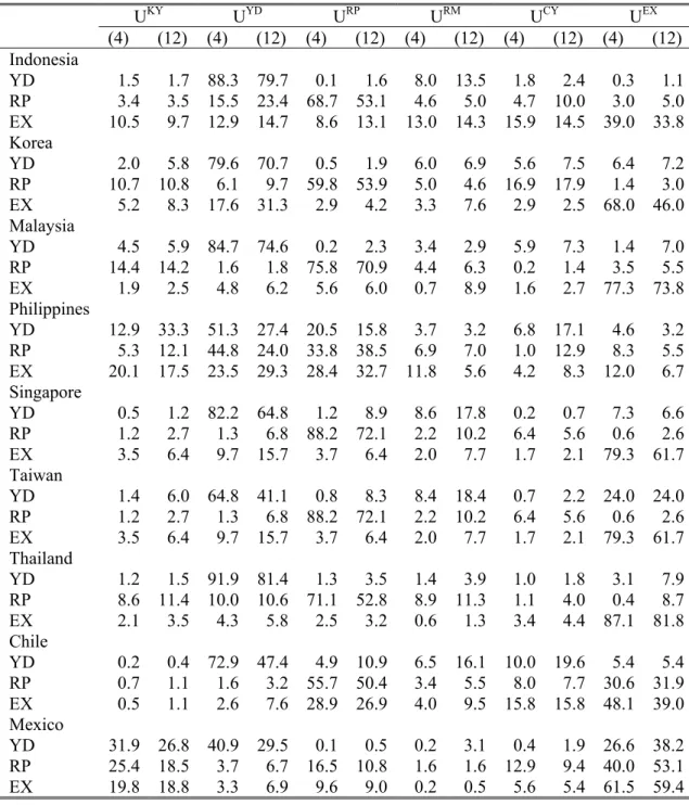
Figure 1 here
Figure 1 shows the real exchange rate (in real line) and output (in dotted line). The nominal and real exchange rates are defined so that an increase denotes depreciation of the domestic currency. We use a trade-weighted exchange rate for all countries other than Mexico, for which the bilateral US dollar rate is used. (See further discussion below.) The Hodrick-Prescott filter is used to eliminate the strong trend in real income data (with λ = 1600). As indicated by the scale of the real exchange rate shown on the right side of the figure, the real exchange is more stable in East Asian countries with the exception of Indonesia.
The case of negative correlation shows up most clearly in Mexico where cyclical
downturns are almost invariably associated with real depreciation. The relative stability of the real exchange rate makes it difficult to read correlation in other countries. In general,
unusually large real depreciation tends to be associated with unusually large decline in real income, the most recent and visible case being the financial crisis of 1997-8 in East Asia.
Theory does not make it clear whether the bivariate relationship is long-term or short-term. The effects of exchange rate changes on income are expected to be temporary since, in the long run, prices adjust proportionately to the change in the nominal exchange rate. The Balassa-Samuelson effect suggests, however, that there may be a negative correlation in the long run. In fast-growing economies like those of East Asian countries, the relative price of nontraded goods would rise faster and thus lead to appreciation of the real exchange rate over time. Existing empirical studies seem to suggest that the above growth effects on the real exchange rate is small or nonexistent in most Asian countries. (Kamin and Klau, 1988; Bahmani-Oskooee, 1998; Upadhyaya,1999)
Table 1 here
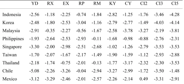
We employ cointegration tests to investigate the nature of long-run relationship. Table 1 reports the results of unit root and cointegration tests. Augmented Dickey Fuller (ADF) tests with 4 lags are used. Variables are defined as follows: YD, domestic real income; RX, the
real exchange rate; EX, the nominal exchange rate; RP, the ratio of the domestic price level to the foreign; RM, real money supply; KY, the capital account-income ratio; CY, the current account-income ratio. (See Appendix 1 for the definition of each variable used in this study.) The results indicate that the presence of unit roots is not rejected for most variables in most countries. In a small number of exceptional cases such as Mexico’s real exchange rate and Chile’s real income, there is evidence that the unit root hypothesis is rejected at the 5 percent significance level.
The last three columns in Table 1 labeled CI2, CI3, and CI5 report the ADF test of cointegration for real income and the real exchange rate. Given the possibility of omitted variables in the cointegration relations, we also report the test results adding foreign income in CI3, foreign income, the capital account-income ratio and real money supply in CI5. In no case, the null hypothesis of noncointegration between output and the real exchange rate is rejected at the 5 percent level. Based on these results, we proceed with the assumption that variables employed here are nonstationary and noncointegrated. Given that the low power of the test and that there is some evidence suggesting the assumption may not be valid, one needs to be cautious and further check on robustness of the results may be necessary.
Table 2 here
The bivariate relationships between the real exchange rate and real income are summarized using cross correlations with leads and lags up to 4 quarters. Since the results turn out to be somewhat sensitive to the method of detrending, we employ 3 different filters: linear detrending, first differencing, and the Hodrick-Prescott filter. The 1997 financial crisis in most East Asian countries constitutes a major structural break in the data. (See Appendix 3 for tests of structural break.) During the period, extremely large devaluations were
accompanied by deep recessions in all countries under study here. To separate the effects of the crisis, we present the results using only the pre-crisis data until the second quarter of 1997 as well as for the whole period.
Another issue in empirical investigation is what exchange rate concept best fits in the study of devaluation. While using the effective exchange rate might be reasonable in most cases, choosing the weights for currencies in the basket can be tricky. Weights based on exports, total trade, trade invoice, and debt contracts can be very different from each other. Appendix 2 summarize the importance of major industrial countries − the U.S., Japan, Western Europe and Germany − in each country’s exports and imports in 1992. Most East Asian countries appear to have fairly diversified trade pattern by 1992, with the U.S., Japan and Western Europe taking roughly equal share in trade in several countries. Exceptional cases are the importance of the U.S. in Malaysian imports and Korean exports. Japan appears to be more important on the import side especially for Malaysia and Thailand. The trade patterns of the two Latin American countries are noticeably different. In Mexico, the U.S. is clearly dominant while Japan and Europe are relegated to minor trading partners. On the other hand, Chile shows the highest portion of trade with European countries among all countries in this study.
We use, as the benchmark case, the bilateral exchange rate against the US dollar. The role of Japan and the yen in East Asia appears almost as important as that of the US and the dollar. In these countries, the prevailing assumption is that the strong yen boosts their economies as their products become more competitive in the world market while the weak yen is associated with difficulties in exports and thus weak economies. (Kwan, 1994; McKinnon, 2000) For these reasons, we employ an effective exchange rate for East Asian countries that is obtained by a simple geometric average of the exchange rate against the US dollar and the exchange rate against the yen. The results are reported under the column “EER”.4 The foreign price level used in defining the real exchange rate is constructed in a parallel manner. For Chile, we use a simple geometric average of the US dollar-, the yen-, and the mark exchange rates. We do not consider the effective exchange rate for Mexico.
4 Although Western Europe as a whole takes a share almost as large as the U.S. or Japan in some cases,
in terms of currency, it is a mixture of many floaters and ERM countries. The latter explain close to half of Western Europe in international trade of East Asian countries.
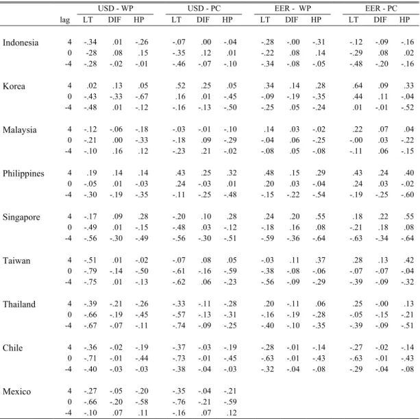
Table 2 reports three representative short-term cross correlations between the real
exchange rate and real income at lags 4, 0, and -4. A positive (negative) lag means the number of quarters by which the real exchange rate leads (lags) real income. The effects of
devaluation on output can be gleaned from correlations at positive lags while correlations at negative lags suggest the extent of reverse causation from real income to the real exchange rate. Correlations at positive lags are clearly negative in the two Latin American countries. In other words, a real devaluation is followed by a cyclical downturn, consistent with the hypothesis of contractionary devaluations. The statistical significance is strongest with the linear trend and much weaker when first differencing is used. As for the East Asian countries, such evidence is quite elusive and depends on the period of estimation and the definition of the real exchange rate. When the US dollar exchange rate is used for the whole period in Case I, there seems strong evidence of contractionary devaluation. Exceptions are noted for Korea, the Philippines, and perhaps, Singapore. It is interesting that the cross correlation at positive lags tends to increase and become positive as the effective exchange rate is used instead of the bilateral dollar rate. Similar changes are observed when the post-crisis period is eliminated in estimation. Thus in Case IV where the effective rate is used for the pre-crisis period, there is no evidence that devaluation is contractionary except possibly the case of Indonesia where the correlation seems insignificantly small anyway. The correlations turn to strongly positive in all other countries. In Chile and Mexico, however, devaluation seems contractionary in the short run regardless of whether the post-1997 data are included or not, and for Chile, whether the US dollar rate or the effective exchange rate is used.
The cross correlations at negative lags, in contrast, appear to be strongly negative in both regions with few exceptions. They are also consistently negative regardless of the sample period and the definition of the exchange rate although such evidence is weaker in Mexico. It suggests that robust economic growth tends to be followed by real appreciation and recession by real depreciation in all these countries.
In sum, Mexico seems to be the only country where the hypothesis of contractionary devaluation appears to be more plausible than the reverse causation hypothesis. For most East Asian countries, the evidence reported in Table 2 is more consistent with the hypothesis in which increases in real income cause appreciation in the real exchange rate than with one in which devaluations cause economic contraction.
Table 3 here
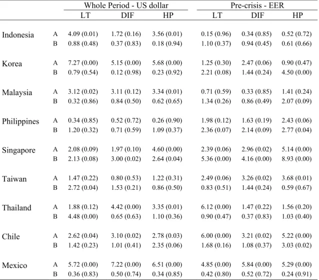
To explore the bivariate relationship further, we report in Table 3 the results of Granger causality tests. In all regressions, we use four lags. For space reasons, we report only two representative cases out of four possible combinations. In Chile and Mexico, there is evidence that the causation is from the real exchange rate to real income than the other way around. It shows up consistently regardless of the sample period or the definition of the exchange rate. In East Asia, Singapore seems to be the only country where the causation from the real exchange rate to output is consistently significant. In this case, the causation from real income to the real exchange rate seems equally strong. In other countries, however, evidence that the observed bivariate correlation is due to causal factors does not seem to be robust. For instance, for Indonesia, Korea, and Malaysia, the real exchange rate Granger-causes real income when the US dollar rate is used (shown in the left columns). However, such evidence disappears when the effective rate is used (shown in the right columns). The opposite holds for Taiwan.
3. The Model
The negative correlation between real income and the exchange rate may arise due to reverse causation and spurious correlation instead of contractionary effects of devalution. Reverse causation from real income to the real exchange rate is likely to be negative especially in fast-growing developing countries where higher income is associated with increases in the relative price of nontraded goods and accompanying appreciation of the real exchange rate over time. Spurious correlation arises where both are affected by some third factors and devaluations usually occur in times of adverse economic conditions. Sharp changes in oil price or capital flows may drive both income and the real exchange rate in opposite directions. In several Latin American countries, exchange rate-based stabilization was a main cause of large capital flows leading to a negative correlation in the two variables. (Kiguel and Liviathan, 1992; Calvo and Vegh, 1993) It is thus important to control for macroeconomic conditions and separate exchange rate changes that may be classified as an exogenous policy shock from those that are reactions to macroeconomic events.
Another weakness of correlation or Granger causality tests is that they cannot explain why devaluation can be contractionary. If small trade elasticities and slow responses in the trade sector are responsible, we should observe that the current account declines with a devaluation. Alternatively, contractionary devaluation may arise due to price shocks that accompany exchange rate changes and the associated increase in the price of imported intermediate and final goods. Unless accommodated by appropriate money supply changes, the price shock reduces real money balance and generates a recessionary pressure by raising the real interest rate. Thus the movements of the price level and real money balance can shed light on the source of contractionary devaluation if it occurs.
In this section, we develop a VAR model to shed some light on the issue raise in the previous section. We consider a 6-variable model that consists of the following variables: capital inflows (
k
t), real income (y
t), the relative price (q
t), real money supply (m
t), the current account balance (c
t), and the nominal exchange rate (e
t). The model also includestwo exogenous variables: foreign real GDP (
y
t*) and the foreign interest rate (i
t*). The 6-variable model with 2 exogenous 6-variables is fairly comprehensive. The six endogenous variables are ordered as listed. Given the evidence reported in the previous section, allvariables are differenced in the model.5 Equation (1) summarizes the model in a compact form:
(1)
+
∆
∆
+
∆
∆
∆
∆
∆
∆
+
=
∆
∆
∆
∆
∆
∆
− − − − − − − − 6 5 4 3 2 1 * 1 * 1 1 1 1 1 1 1 6 5 4 3 2 1)
(
)
(
t t t t t t t t ij t t t t t t ij t t t t t ti
y
L
B
e
c
m
q
y
k
L
A
e
c
m
q
y
k
ε
ε
ε
ε
ε
ε
µ
µ
µ
µ
µ
µ
where
A
ij(L
)
andB
ij(L
)
are 6×6 and 6×2 matrices of polynomials in lag operatorL
.Several features of the model can be noted. First, external shocks are explicitly
incorporated. (We tried additional variables such as the terms of trade but dropped them as they make little qualitative differences in results.) Second, capital flows are treated as a driving force of the macroeconomic variables. The placement of the variable at the top of the endogenous variables reflects the assumption that, in the short run, it is largely determined by external factors. (See, for supporting evidence, Calvo et al. 1993.) Third, the real exchange rate is decomposed into the nominal exchange rate and the relative price. A country may have some control over the nominal exchange rate. However, the real exchange rate is determined by factors such as productivity growth and thus cannot be controlled except in the short run. Moreover, devaluation often fails as resulting increases in the price level erode competitive advantage generated by the change in the nominal exchange rate. With the setup, we can study the effects of a nominal devaluation on the relative price and therefore on the real exchange rate. Fourth, the real money balance is included since changes in the money supply may determine the short-term results of devaluation. The effects of devaluation crucially
5 VAR models have been employed in related contexts. Rogers and Wang (1995) show that
devaluations lead to output declines in Mexico; Copelman and Werner (1996) introduce credit channels as a potential link to contractionary devaluations; Hoffmaister and Vegh (1996) find that a permanent reduction in the exchange rate depreciation leads to a long-lasting increase in output. See
depend on monetary and fiscal policies that accompany it. The behavior of the real money supply can be an important key to the understanding the effects of devaluation.
Fifth, the current account is included as well as the capital account. Most countries included in this study eliminated capital controls and liberalize capital account transactions only recently. During the bulk of the sample period, shocks to the current account such as terms of trade shocks were the main shock to the balance of payments. Moreover, due to heavy intervention in the foreign exchange market, the two accounts were strongly related but not identical with opposite signs. By placing the current account above the nominal exchange rate, we can also narrow the range of exchange rate shocks so that they do not include
contemporaneous reactions to developments in the balance of payments from both capital and current account sources.
One of the most important differences between this model and the models adopted in the previous studies would be that the nominal exchange rate is placed at the bottom. The ordering is based on the observation that the exchange rate, as a forward-looking asset price, responds quickly to macroeconomic shocks. For instance, the exchange rate authority may respond to adverse shocks to the current account by letting the domestic currency depreciate. Similarly, favorable productivity shocks may lead the authority to allow its appreciation. In this setup, these contemporaneous (endogenous) changes in the exchange rate due to other variables in the system are taken care of and excluded from exchange rate shocks. What remains after accounting for those endogenous responses can be termed exchange rate shocks. They may be called exogenous changes in the exchange rate that are the subject of a
devaluation study.6 This is adapted from the methodology of Kim and Roubini (2000) who employed a similar methodology in their study of monetary policy effects and accounted for
Kamin and Rogers (2000) for a comprehensive study with the Mexican data as well as an excellent survey of recent literature.
6 The exchange rate is often placed at or near the top of ordering on the grounds that empirical studies
have found that it is not well explained by other variables. For instance, Kamin and Rogers (2000) place the real exchange rate near the top after external variables such as the foreign (U.S.) interest rate and the terms of trade. In such models, innovations from the exchange rate equation are likely to include adverse shocks to the economy such as deterioration in the terms of trade, leading to spurious correlation.
various puzzles in existing studies. The idea is that the exchange rate, as a forward-looking asset price, is contemporaneously affected by other variables such as income, prices and the balance of payments. The assumption appears reasonable in our case since most countries studied in this paper have maintained some sort of managed floating in which the exchange rate is adjusted in response to the economic condition.
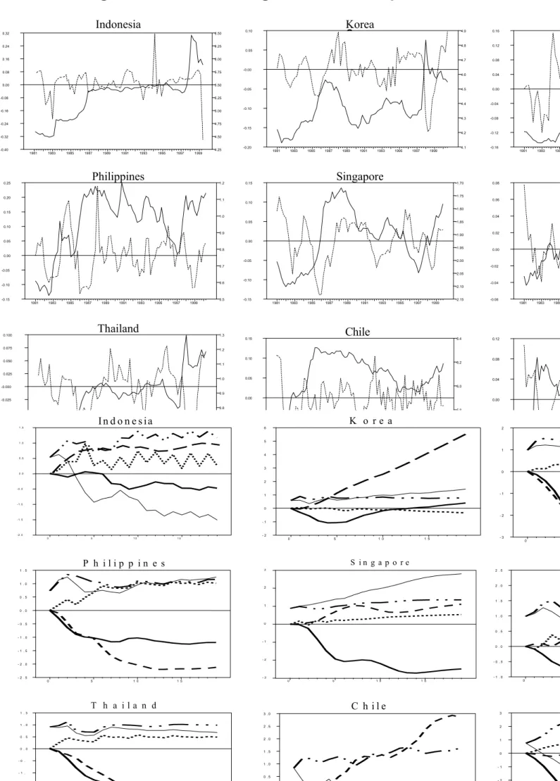
Figure 2 here Figure 3 here
Panels in Figures 2 and 3 show the impulse responses to an increase in the nominal exchange rate (shown in double-dotted line). In addition to the response of output (in thick real line), responses of the real exchange rate (thin real line), the current account (dotted line), and the real money supply (broken line). Although the model is estimated in the first
difference form, the variables are converted back to levels in impulse responses.
As noted in the above, the effects of the dollar exchange rate are very different from those of the effective rate. Also, due to the structural break in the series induced by the financial crisis, it is not clear which, between the whole sample and the pre-crisis period, better represents the economies in East Asia. There is strong evidence of structural breaks in most variables in the system in all crisis-stricken economies. (See Appendix 3.) Out of four possible combinations, we present two cases: one with the US dollar and the whole period in Figure 2 and the other with the effective rate and the pre-crisis in Figure 3. The other two cases that are not presented here lie between the two that are shown. (For Mexico, the two cases are identical since the case with the effective rate is not considered separately. The US dollar rate is used in both figures.)
According to Figure 2, a devaluation is unambiguously contractionary in all nine
countries. The case of Mexico has been well documented. See Kamin and Rogers (2000) for a recent study. Figure 2 suggests that devaluation leads to similar results in other countries as well. In the Philippines, Singapore and Thailand, the recessionary effects of devaluation appear to be persistent. In Korea, Taiwan, and Chile, they seem to be reversed to
expansionary effects in two to three years. In Indonesia, the contractionary effects seem to kick in with some delay.
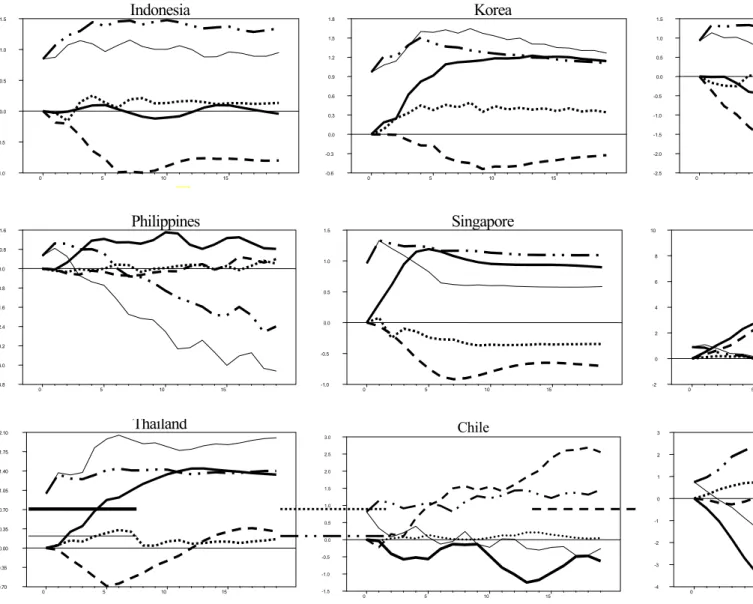
Panels in Figure 3, in sharp contrast to those in Figure 2, suggest that devaluation of the
effective exchange rate in the pre-crisis period has been contractionary in no East Asian
countries. On the contrary, devaluation seems to be strongly expansionary in all countries but Indonesia and Malaysia where the output effects appear small and insignificant. Moreover, the expansionary effects seem to be persistent and supported by persistent depreciation of the real exchange rate after devaluation. In a remarkable contrast, devaluation continues to be equally contractionary in the two Latin American countries. The comparison of the two figures also suggests that the 1997 crisis did not constitute a major structural break for Latin American countries. (See Appendix 3 for supporting evidence.) For Chile, using the effective exchange rate makes little difference except that initial effects appear somewhat smaller.7 It then follows that the possibility of contractionary devaluation is more general for Chile and Mexico whereas, in East Asia, it is limited to the US dollar exchange rate (and the inclusion of the crisis episode).
A closer inspection of Figure 2 reveals that sources of contractionary devaluations differ across countries. In Chile and Mexico, the real exchange rate falls below the pre-devaluation level within a few quarters after devaluation. In these cases, appreciation of the real exchange rate seems to be the main cause of the contractionary pressure after devaluation. The two countries have employed the exchange rate as an anchor in a number of attempts to reduce inflation, in which the rate of currency devaluation was kept at a level lower than the
7
If the pre-crisis sample is used along with the US dollar rate (not shown here), contractionary devaluation is found (as in the whole period) in Singapore, Thailand, Taiwan as well as Chile and Mexico. In the other countries, effects are weak or initial contractionary effects are reversed (or vice versa). In no countries, however, devaluation seems to be expansionary. On the other hand, when the whole period is used along with the effective rate (not shown), there is evidence of contractionary devaluation for Indonesia, Malaysia, and the Philippines while a devaluation is followed by output expansion in Korea, Singapore, Taiwan (and very weakly, in Thailand). It seems that, in the first three countries, the structural break associated with the 1997 crisis pulls the results to the direction in which devaluation is associated with weak output performance. One could say that the use of the US dollar rate is a bit more responsible for the finding of contractionary devaluations while, for Indonesia, Malaysia, and the Philippines, it is the weight of the recent crisis that produces the results.
differential between domestic and foreign inflation rates. With strong inflation inertia, the real exchange rate started appreciating soon after devaluation episodes, thereby building up the recessionary pressure as the traded sector of the economy loses competitiveness. In East Asia, Indonesia − perhaps the only East Asian country that has had inflation problems similar to that of Chile and Mexico − seems to follow this pattern. In all the other countries, the real exchange rate and the nominal exchange rate follow similar paths, suggesting that currency devaluation has not been undermined by price increases for a significant length of time.
In Malaysia, the Philippines, and Thailand, the real money supply sharply declines with devaluation. In those countries, contractionary devaluation seems to arise mainly from conservative (unaccommodating) monetary policy that accompanies devaluation. Figure 3 suggests, however, that tight monetary policy was not entirely responsible for the outcome given that devaluation leads to output expansion despite sustained reduction in real money supply in several other countries. In Korea and Taiwan, contractionary devaluation seems mainly a short-term phenomenon, lasting less than 10 quarters and then reverting to expansionary effects afterwards.8
It is important to note that, in both sets of figures, the current account almost invariably improves after devaluation. This is true even for Chile and Mexico where there is strong and consistent evidence that devaluation causes contractionary influences. Singapore is the only exception where the current account deteriorates slightly. It suggests that, whether
devaluation is contractionary or expansionary may have little to do with the trade elasticities condition.
Table 4 here Table 5 here
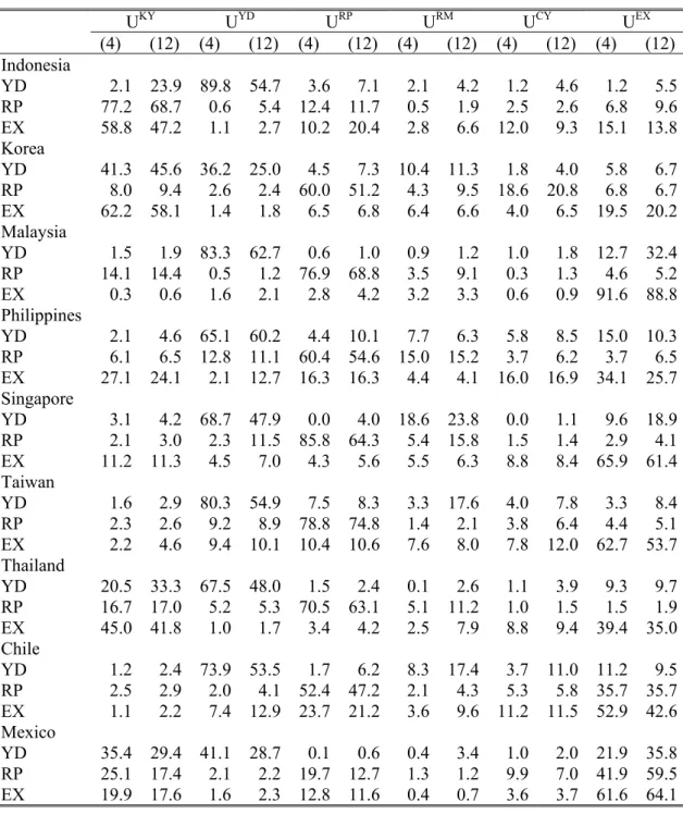
In Tables 4 and 5, we present two sets of variance decomposition for the two same combinations of the exchange rate definitions and the sample period. Ui denotes innovations
8 Singapore is unique in that economic contraction is persistent and shows no sign of reversal. Our
model is unable to explain such tendency. Perhaps, real income is determined entirely independent of exchange rate movements while the domestic currency weakens at the sign of recession. The two recessions in the data during 1985-5 and 1997-8 were accompanied by sharp currency depreciation.
from the equation for variable i. For space reasons, variance decompositions of only 3 variables are reported: output, the relative price, and the nominal exchange rate. A
comparison of the two tables indicates that the causes of movements for the exchange rate are quite different depending on the period and the definition of the exchange rate. For the effective exchange rate, Table 5 suggests that own shocks are most important (with the exception of the Philippines). Shocks to income are the distant second in explaining the exchange rate. Other than shocks to income, no variables seem to be consistently related to exchange rate shocks. The results suggest that the exchange rate authorities of these countries have used the exchange rate as a stabilization tool, allowing it to adjust to business conditions while trying to maintain the effective exchange rate stable. As far as the US dollar exchange rate is concerned for the whole period (shown in Table 4), capital flows take a major role in all cases. In Indonesia, Korea and Thailand, the capital account is the most important variable that explains the exchange rate behavior. Malaysia and Chile − and, perhaps, Taiwan − are interesting exceptions. Malaysia and Chile are well known to have used capital controls in times of exchange rate crises, which have presumably helped to maintain stability in the middle of financial turmoil. As a consequence, variations in capital flows have minimal effects on the exchange rate in these cases.
For domestic output, own shocks are the most important one in all cases. In the precrisis East Asia (Table 5), output is little affected by the exchange rate in any East Asian countries except Taiwan. Also, capital flows play a small role for all but the Philippines. These results suggest that East Asian countries during the pre-crisis period may well be described as “insular.” Even though the export-driven economic growth has significantly opened up the economy and raised the extent of dependence on foreign economic conditions, interest rate and foreign exchange controls and various other impediments on capital flows seem to have rendered them to largely insensitive to external shocks.9 In contrast, Table 4 reports that
9 Note that our model includes two exogenous variables, foreign output and the foreign interest rate.
external variables are far more important for output when the US dollar rate is used for the whole period. The increase in the importance of capital flows is clear in Indonesia, Korea, Thailand, and Mexico. Malaysia and Singapore show a greater role of the exchange rate.
5. Conclusion
In this paper, we investigated whether a devaluation is likely to be contractionary on domestic output in East Asian countries as it is in Latin American countries with surprising consistency suggested in many existing studies. We employed quarterly data for the last two decades. Summarizing main results: historically, devaluation is closely associated with recession in both groups of countries. A closer inspection reveals, however, that the negative correlation may be due to reverse causation especially in East Asian countries in which strong income growth has preceded appreciation of the real exchange rate. The effects of devaluation seem very different depending on the period of estimation and the definition of the exchange rate, however. When the effective rate is used for the pre-1997 crisis period, there is little evidence of contractionary devaluation in East Asia. In fact, in more than half the cases, a devaluation leads to a persistent output expansion. This is sharply contrasted to the case of Mexico and, somewhat weakly, Chile, where there is strong evidence that a devaluation leads to temporary reduction in output.
The results also suggest that contractionary devaluation cannot be ruled out in East Asia. They indicate that devaluation in terms of the US dollar exchange rate is likely to be
contractionary in East Asian countries just as well as in Mexico and Chile especially when the post-crisis data are included in estimation. No doubt the inclusion of the dramatic episode tilts the results towards such results. Our exercise suggests the crisis period indeed was different. With financial liberalization and tremendous improvement in information technology, devaluation may be more likely to be contractionary than before as it worsens the balance sheet of financial and nonfinancial business firms with heavy foreign-currency liabilities and
the variations in capital flows. Thus when their effects are taken into consideration, little is left to capital flows.
results in serious interruption of external financing through a loss of credibility with
international financial investors. It is too early to determine whether this new paradigm is here to stay for East Asian countries. One must exercise due care in interpreting the results for the period including financial crises since the exchange rate - output linkage can be complicated by many abnormal factors such as contagion and self-fulfilling expectations.
Policy implications of the finding of this paper are significant. First of all, when
the trade pattern is as diverse as in East Asian countries, it matters a great deal how
the exchange rate is defined. Due to the international role of the dollar and due to the
fact that it is closely watched by investors, the dollar exchange rate is certainly
important for all countries. However, devaluation in terms of the dollar may bring
contractionary effects in East Asian countries. It may be the recognition of such a
perverse outcome that has lead virtually all East Asian countries to soft dollar pegging
similar to their past policy soon after the worst moment of the crisis is over.
(McKinnon, 2000) For them, devaluation of the dollar exchange rate may no longer
be an effective tool of economic stabilization. On the other hand, the exchange rate
against the yen plays a more regular function as expected in the textbook. As a gauge
of international competitiveness against the major competitor in the world market,
devaluation against the yen promotes the traded goods sector and boosts economic
activity. The perverse effects of devaluation through adverse supply-side effects or
credit channels do not seem to be dominant as in the case of the dollar exchange rate.
This is surprising given that substantial amounts of foreign debt are denominated in
yen and Japan is the major source of intermediate inputs in many East Asian countries.
For those countries that have returned to the soft-dollar pegging, the regular and more
expected effects of the yen exchange rate do not mean much consolation since it is
beyond the control as they choose to stabilize their currency against the dollar. Instead,
the gyrations of the yen-dollar exchange rate as observed in the past decade pose a
serious challenge to the exchange rate policy.
Appendix 1: Data and definitions
The domestic price level is measured by the consumer price index (CPI) and real income by industrial production or, in Taiwan, real GDP. Most real income series are deseasonalized by removing the effects of seasonal terms in a simple regression containing a linear trend and seasonal dummies. For the money supply, the M2 concept is used. The capital (current) account-income ratio, KY (CY), is obtained as the ratio of the capital (current) account balance to the trend nominal GDP. If the balance of payments statistics are unavailable, the current account balance is approximated by the difference between merchandise exports and imports. The capital account, in turn, is approximated by first obtaining the difference in net foreign assets at the central bank (which is considered the official reserve balance) and then subtracting the current account from it. The log of trend nominal GDP is assumed to be linear in trend. For nominal income series, we use nominal GDP if available. Otherwise, it is
approximated by the product of real income and the domestic price level, both defined above. Foreign real income and the foreign price level are measured by real GDP and the CPI of the US. The US 3-month Treasure Bill interest rate is used as foreign interest rate. For EER, the simple geometric average of the US and Japan (the US, Japan, and Germany) is used as the foreign country in East Asian countries (Chile). All variables are in logarithm except the interest rate and the CY and KY ratios.
The sample periods are: Indonesia (1981:1-1999:2), Korea (1980:1-2000:3), Malaysia (1970:1-2000:1), Philippines 2000:2), Singapore (1970:1-1999:4), Taiwan (1981:1-2000:3), Thailand (1976:1-2000:2), Chile (1972:4-(1981:1-2000:3), and Mexico (1981:1-2000:2). Taiwan’s data are extracted from Aremos databank. All other data are obtained from International Financial Statistics (CR-ROM).
Appendix 2: Trade Patterns
Share of Export Share of Imports
IC U.S. Japan Europ
e Ger IC U.S. Japan Europe Ger
Indonesia 65.9 13.7 34.3 14.3 3.1 63.1 11.1 22.2 22.9 7.9 Korea 97.6 23.7 15.1 13.5 3.8 99.5 22.4 23.8 13.8 4.6 Malaysia 50.6 18.7 13.3 16.1 4.0 61.1 15.9 46.0 15.3 4.2 Philippines 81.9 40.0 19.7 19.1 6.4 60.5 18.7 23.7 14.2 4.3 Singapore 45.9 21.2 5.7 15.7 4.4 54.1 15.8 21.6 15.3 3.4 Taiwan 51.8 28.9 10.9 16.8 4.4 64.4 21.9 30.2 16.3 5.5 Thailand 64.8 22.5 17.5 21.8 4.4 62.0 11.7 29.3 17.4 5.3 Chile 64.0 16.6 15.9 30.4 5.9 55.2 20.4 9.9 22.6 6.5 Mexico 92.6 76.4 2.6 8.4 1.2 91.2 69.3 6.5 14.0 4.8
Note: Calculated using 1992 annual exports and imports data obtained from Direction of
Appendix 3: Tests of Structural Break
Tests of Structural Break
DF1 DF2 Y EX RP RM KY CY Indonesia 8 37 0.38 19.6** 9.74** 2.29+ 112** 3.13* 0.42 18.7** 5.52** 2.27+ 101** 4.22* Korea 13a 46a 0.72 61.5** 4.38** 4.47** 10.1** 4.15** 2.07+ 13.8** 3.88** 3.85** 7.88** 2.72* Malaysia 11 84 1.07 11.9** 0.23 1.11 0.89 2.34+ 1.47 5.71** 0.21 1.47 1.05 2.45+ Philippines 11a 30a 9.83** 3.20* 5.14** 0.96 4.34** 1.20* 11.4** 2.72* 2.89* 0.84* 4.26* 1.51 Singapore 10 83 0.72 4.26** 0.12 4.89** 1.74 1.61 1.11 2.92* 0.42 4.01* 1.55 1.84 Taiwan 13 42 1.20 3.95* 1.04 0.59 0.99 0.67 1.29 1.00 1.06 1.23 0.99 0.61 Thailand 12 64 0.78 14.0** 2.18* 1.54 5.15** 2.95* 1.63 5.14** 2.59* 1.60 6.68** 3.38* Chile 13 61b 0.74 0.39 0.51 1.30 0.16 0.11 Mexico 12 49 0.56 0.50 0.43 0.48 0.38 0.50
Note: Reported are the F-statistics for the Chow predictive tests. DF1 and DF2 are the degrees of freedom for the numerator and the denominator. ‘a’ denotes that the degrees of freedom for KY and CY (and also DF2 of RM for the Philippines) are lower by 1. In case of Chile (‘b’ ), the degree of freedom is 60 for RM and KY. ‘+’, ‘*’ and ‘**’ denote significance at the 10, 5 , and 1 percent level, respectively.
References
Bahmani-Oskooee, Mohsen. Are Devaluations Contractionary in LDCs? Journal of Economic
Development. Vol. 23 (1). p 131-44. June 1998.
Buffie, Edward F. 1989. Imported inputs, real wage rigidity and devaluation in the small open economy. European Economic Review. 33(7): 1345-61.
Calvo, G., Vegh, C.A., 1993. Exchange rate based stabilization under imperfect credibility. In: Frisch H., Worgotter, A. (Eds.), Open Economic Macroeconomics. MacMillan, London, pp. 3-28.
Calvo, Guillermo, Leonardo Leiderman, and Carmen M. Reinhart, “Capital Inflows and Real Exchange Rate Appreciation in Latin America,” IMF Staff Papers 40 (March 1993), 108-151.
Cooper, Richard, “Currency Depreciation in Developing Countries,” Princeton Essays in
International Finance 86 (1971).
Corsetti, G., P. Pesenti, and N. Roubini, “What Caused the Asian Currency and Financial Crisis?” Japan and the World Economy 11 (1999), 305-373.
Diaz-Alejandro, C.F., 1963. A note on the impact of devaluation and the redistributive effects,
Journal of Political Economy 71. 577-580.
Domac, Ilker. Are Devaluations Contractionary? Evidence from Turkey. Journal of Economic
Development. Vol. 22 (2). p 145-63. December 1997.
Dornbusch, R. and Y. C. Park, “Flexibility or Nominal Anchor?” in Stefan Collignon, Jean Pisani-Ferry and Yung Chul Park (eds), Exchange Rate Policies in Emerging Asian
Countries (London: Routledge, 1999), 3-34.
Edwards, Sebastian, “Are Devaluations Contractionary?” Review of Economics and Statistics 68 (1986), 501-508.
_____, Real Exchange Rates, Devaluation, and Adjustment (MIT Press: Cambridge, MA, 1989)
Eichengreen, Barry and Jeffrey Sachs, “Exchange Rates and Economic Recovery in the 1930s,” Journal of Economic History 44 (December 1985), 925-946.
Findlay, Roland and Carlos Alfredo, Rodriguez (1977). “Intermediated imports and macroeconomic policy under flexible exchange rates. Canadian Journal of Economics 10(2):208-17.
Frankel, J. A. “Ambiguous Policy Multipliers in Theory and in Empirical Models,” Ralph C. Bryant, et al. (eds.) Empirical Macroeconomics for Interdependent Economies
(Washington, DC: Brookings Institution, 1988), 17-26.
Frankel, J. A. and A. Rose, “Fixing Exchange Rates: A Virtual Quest for Fundamentals,”
Goldstein, Morris, and Mohsin S. Khan, “Income and Price Effects in Foreign Trade,” in
Handbook of International Economics, Vol. II, edited by Ronald W. Jones and Peter B.
Kenen (Amsterdam: North-Holland, 1985), 1041-1105.
Gordon, Robert J. “The Aftermath of the 1992 ERM Breakup: Was There a Macroeconomic FreeLunch?” P. Krugman, (ed.) Currency Crises (Chicago: National Bureau of Economic Research, 2000).
Gylfasson, T. and O. Risager, “Does Devaluation Improve the Current Account?” European
Economic Review 25 (1984), 37-64.
Gylfasson, T. and M. Schmid, “Does Devaluation Cause Stagflation?” Canadian Journal of
Economics 16 (1983), 641-654.
Hallett, A J Hughes; Wren-Lewis, S. Is There Life Outside the ERM? An Evaluation of the Effects of Sterling's Devaluation on the UK Economy. International Journal of Finance &
Economics. Vol. 2 (3). p 199-216. July 1997.
Hoffmaister, A.W., Vegh, C., 1996. Disinflation and the recession-now-versus-recession-later hypothesis: evidence from Uruguay. IMF Staff Papers 43, 355-394.
Kamas, Linda. Devaluation, National Output and the Trade Balance: Some Evidence from Colombia. Weltwirtschaftliches Archiv-Review of World Economics. Vol. 128 (3). 425-45. 1992.
Kamin, Stevel B and John Rogers H. 2000. Output and the real exchange rate in developing countries: an application to Mexico. Journal of Development Economics. 61(1): 85-109. Kamin, Steven B; Klau, Marc. Some Multi-Country Evidence on the Effects of Real
Exchange Rates on Output. Board of Governors of the Federal Reserve System, International Finance Discussion Papers: 611. p 18. May 1998.
Kiguel, M. and N. Liviathan. “The Business Cycle Associated with Exchange Rate Based Stabilization.” World Bank Economic Review 6 (1992), 279-305.
Krugman, P. “Balance Sheets, the Trasnsfer Problem, and Financial Crises,” unpublished (January 1999), MIT.
Krugman, P., and L. Taylor, “Contractionary Effects of Devaluation,” Journal of
International Economics 8 (August 1978), 445-456.
Kwan, C. H., Economic Interdependence in the Asia-Pacific Region (London: Routledge, 1994).
Lizondo, S. and Montiel, P.J., 1989, Contractionary devaluation in developing countries: an analytical overview. IMF Staff Papers 36, 182-227.
Marston, R. C. (1982) “Wages, relative prices and the choice between fixed and flexible exchange rates” Canadian Journal of Economics 15(1): 87-103.
McKinnon, Ronald I. “After the Crisis, the East Asian Dollar Standard Resurrected: An Interpretation of High-Frequency Exchange Rate Pegging,” Department of Economics, Stanford University, (August 2000).
Morley, Samuel A. 1997. On the effect of devaluation during stabilization programs in LDCs.
Review of Economic & Statistics. 74(1): 21-27.
Obsteld, M. and K. Rogoff, “The Mirage of Fixed Exchange Rates,” Journal of Economic
Perspectives 9 (Fall 1995), 73-96,
Reinhart, C. M. “The Mirage of Floating Exchange Rates,” American Economic Review 20 (May 2000)
Rogers, J.H., Wang, P., 1995. Output, inflation, and stabilization in a small open economy: evidence from Mexico. Journal of Development Economics 46, 271-293.
Sachs, Jeffery. (1980) “Wages, flexible exchange rates, and macroeconomic policy”
Quarterly Journal of Economics 94(4):731-47.
Schnedier, Martin and Aaron Tornell, “Balance Sheet Effects, Bailout Guarantee and Financial Crises,” NBER Working Paper 8060 (December 2000).
Solimano, A. “Contractionary Devaluation in the Southern Cone: The Case of Chile,” Journal
of Development Economics 23 (September 1986), 135-151.
Upadhyaya, Kamal P., “Currency devaluation, aggregate output, and the long run: an empirical study,” Economics Letters 64 (1999), 197-202.
Williamson, J. “The Case for a Common Basket Peg for East Asian Currencies?” in Stefan Collignon, Jean Pisani-Ferry and Yung Chul Park (eds), Exchange Rate Policies in
Emerging Asian Countries (London: Routledge, 1999), 327-343.
Williamson, J. Exchange Rate Regimes for Emerging Markets: Reviving the Intermediate
Table 1: Unit Root and Cointegration Tests
YD RX EX RP RM KY CY CI2 CI3 CI5
Indonesia -2.56 -1.18 -2.25 -0.74 -1.84 -2.82 -1.25 -1.76 -3.46 -4.28 Korea -2.48 -1.80 -2.53 -3.04 -1.16 -2.79 -2.77 -1.49 -4.03 -4.14 Malaysia -2.91 -0.35 -2.27 -0.56 -1.67 -2.58 -3.78 -3.27 -2.19 -3.81 Philippines -1.93 -2.64 -2.53 -2.93 -0.11 -1.68 -0.98 -0.88 -2.76 -2.31 Singapore -3.30 -2.00 -2.98 -2.51 -2.68 -1.02 -1.26 -2.79 -3.53 -3.53 Taiwan -1.70 -2.07 -1.67 -2.17 -1.49 -1.90 -1.59 -1.12 -2.93 -2.88 Thailand -2.18 -1.74 -0.75 -2.01 -0.13 -1.77 -3.17 -2.32 -2.30 -3.53 Chile -5.08 -2.26 -3.26 -0.04 -2.94 -3.27 -2.99 -1.72 -3.50 -1.48 Mexico -3.12 -3.29 -2.46 -2.01 -2.57 -2.26 -2.14 0.49 -3.31 -2.91 Note: Reported are Augmented Dickey Fuller unit-root tests with 4 lags. CI2 and CI3 are cointegration tests with (YD, RX) and {YD, RX, YF}, respectively. CI5 is an expanded model with {YD, RX, YF, KY, RM}. For the real and nominal exchange rates, the effective exchange rate is used for the East Asian countries and the bilateral US dollar rate for Chile and Mexico.
Table 2: Cross Correlations
USD - WP USD - PC EER - WP EER - PC lag LT DIF HP LT DIF HP LT DIF HP LT DIF HP
Indonesia 4 -.34 .01 -.26 -.07 .00 -.04 -.28 -.00 -.31 -.12 -.09 -.16 0 -28 .08 .15 -.35 .12 .01 -.22 .08 .14 -.29 .08 .02 -4 -.28 -.02 -.01 -.46 -.07 -.10 -.34 -.08 -.05 -.48 -.20 -.16 Korea 4 .02 .13 .05 .52 .25 .05 .34 .14 .28 .64 .09 .33 0 -.43 -.33 -.67 .16 .01 -.45 -.09 -.19 -.35 .44 .11 -.04 -4 -.48 .01 -.12 -.16 -.13 -.50 -.25 .05 -.24 .01 -.01 -.52 Malaysia 4 -.12 -.06 -.18 -.03 -.01 -.10 .14 .03 -.02 .22 .07 .04 0 -.21 .00 -.33 -.18 .09 -.29 -.04 .06 -.25 -.00 .03 -.22 -4 -.10 .16 .12 -.23 .21 -.02 -.08 .05 -.08 -.11 .06 -.15 Philippines 4 .19 .14 .14 .43 .25 .32 .48 .15 .29 .43 .24 .40 0 -.05 .01 -.03 .24 -.03 .01 .20 .03 -.04 .24 .03 -.02 -4 -.30 -.19 -.35 -.11 -.25 -.48 -.15 -.22 -.54 -.19 -.25 -.60 Singapore 4 -.17 .09 .28 -.20 .10 .28 .24 .20 .55 .18 .22 .55 0 -.49 .01 -.15 -.48 .03 -.12 -.18 .16 .08 -.21 .18 .08 -4 -.56 -.30 -.49 -.56 -.30 -.51 -.59 -.36 -.64 -.63 -.34 -.64 Taiwan 4 -.51 .01 -.02 -.07 .08 .05 -.03 .11 .37 .28 .13 .42 0 -.79 -.14 -.50 -.61 -.16 -.59 -.38 -.08 -.06 -.07 -.07 -.04 -4 -.75 .01 -.13 -.62 .06 -.23 -.56 -.09 -.29 -.39 -.09 -.32 Thailand 4 -.39 -.21 -.26 -.33 -.11 -.28 .20 -.11 .06 .25 -.00 .13 0 -.66 -.19 -.45 -.57 -.13 -.31 -.16 -.19 -.28 -.05 -.15 -.21 -4 -.67 -.07 -.11 -.74 -.09 -.25 -.40 -.10 -.35 -.39 -.09 -.51 Chile 4 -.36 -.02 -.19 -.37 -.03 -.19 -.28 -.01 -.14 -.27 -.02 -.14 0 -.71 -.01 -.44 -.73 -.01 -.45 -.63 -.01 -.43 -.63 -.01 -.43 -4 -.40 -.03 -.03 -.38 -.04 -.03 -.32 -.04 -.08 -.29 -.04 -.08 Mexico 4 -.27 -.05 -.20 -.35 -.04 -.21 0 -.66 -.20 -.58 -.76 -.21 -.59 -4 -.10 .07 .11 -.16 .07 .12
Note: Reported are the cross correlations of real exchange rate and detrended real income and at lag k. A positive (negative) lag represents the number of quarters by which the real
exchange rate leads (lags) real income. USD refers to the case where the US is considered as the foreign country. For EER, the simple geometric average of the US and Japan (the US, Japan, and Germany) is used as the foreign country in East Asian countries (Chile).
Table 3: Granger Causality Tests
Whole Period - US dollar Pre-crisis - EER
LT DIF HP LT DIF HP Indonesia A 4.09 (0.01) 1.72 (0.16) 3.56 (0.01) 0.15 (0.96) 0.34 (0.85) 0.52 (0.72) B 0.88 (0.48) 0.37 (0.83) 0.18 (0.94) 1.10 (0.37) 0.94 (0.45) 0.61 (0.66) Korea A 7.27 (0.00) 5.15 (0.00) 5.68 (0.00) 1.25 (0.30) 2.47 (0.06) 0.90 (0.47) B 0.79 (0.54) 0.12 (0.98) 0.23 (0.92) 2.21 (0.08) 1.44 (0.24) 4.50 (0.00) Malaysia A 3.12 (0.02) 3.11 (0.12) 3.34 (0.01) 0.71 (0.59) 0.33 (0.85) 1.41 (0.24) B 0.32 (0.86) 0.84 (0.50) 0.62 (0.65) 1.34 (0.26) 0.86 (0.49) 2.07 (0.09) Philippines A 0.34 (0.85) 0.52 (0.72) 0.26 (0.90) 1.98 (0.12) 1.63 (0.19) 2.43 (0.06) B 1.20 (0.32) 0.71 (0.59) 1.09 (0.37) 2.36 (0.07) 2.14 (0.09) 2.77 (0.04) Singapore A 2.08 (0.09) 1.97 (0.10) 4.60 (0.00) 2.39 (0.06) 2.96 (0.02) 5.14 (0.00) B 2.13 (0.08) 3.00 (0.02) 2.64 (0.04) 5.36 (0.00) 4.16 (0.00) 8.93 (0.00) Taiwan A 1.47 (0.22) 0.80 (0.53) 1.22 (0.31) 2.49 (0.06) 3.26 (0.02) 3.68 (0.01) B 2.72 (0.04) 1.53 (0.21) 0.86 (0.50) 0.83 (0.51) 1.44 (0.24) 0.59 (0.67) Thailand A 1.88 (0.12) 4.42 (0.00) 3.35 (0.01) 6.12 (0.00) 1.47 (0.22) 1.56 (0.20) B 4.48 (0.00) 0.65 (0.63) 1.10 (0.36) 0.90 (0.47) 0.37 (0.83) 1.03 (0.40) Chile A 2.62 (0.04) 3.10 (0.02) 2.78 (0.03) 6.00 (0.00) 3.21 (0.02) 5.22 (0.00) B 1.42 (0.23) 1.01 (0.41) 2.35 (0.06) 1.68 (0.16) 1.08 (0.37) 3.03 (0.02) Mexico A 5.72 (0.00) 7.22 (0.00) 6.51 (0.00) 4.85 (0.00) 5.84 (0.00) 5.29 (0.00) B 0.36 (0.83) 0.50 (0.74) 0.34 (0.85) 0.42 (0.80) 0.52 (0.72) 0.24 (0.91)
Note: Reported are F-statistics with P values inside the parentheses. Row A tests the
hypothesis that the real exchange rate Granger causes real income. Row B tests the hypothesis that real income Granger causes the real exchange rate. For Chile and Mexico, the US dollar exchange rate is used in place of the effective rate.
Table 4: Variance Decomposition (Whole period, US dollar) UKY UYD URP URM UCY UEX (4) (12) (4) (12) (4) (12) (4) (12) (4) (12) (4) (12) Indonesia YD 2.1 23.9 89.8 54.7 3.6 7.1 2.1 4.2 1.2 4.6 1.2 5.5 RP 77.2 68.7 0.6 5.4 12.4 11.7 0.5 1.9 2.5 2.6 6.8 9.6 EX 58.8 47.2 1.1 2.7 10.2 20.4 2.8 6.6 12.0 9.3 15.1 13.8 Korea YD 41.3 45.6 36.2 25.0 4.5 7.3 10.4 11.3 1.8 4.0 5.8 6.7 RP 8.0 9.4 2.6 2.4 60.0 51.2 4.3 9.5 18.6 20.8 6.8 6.7 EX 62.2 58.1 1.4 1.8 6.5 6.8 6.4 6.6 4.0 6.5 19.5 20.2 Malaysia YD 1.5 1.9 83.3 62.7 0.6 1.0 0.9 1.2 1.0 1.8 12.7 32.4 RP 14.1 14.4 0.5 1.2 76.9 68.8 3.5 9.1 0.3 1.3 4.6 5.2 EX 0.3 0.6 1.6 2.1 2.8 4.2 3.2 3.3 0.6 0.9 91.6 88.8 Philippines YD 2.1 4.6 65.1 60.2 4.4 10.1 7.7 6.3 5.8 8.5 15.0 10.3 RP 6.1 6.5 12.8 11.1 60.4 54.6 15.0 15.2 3.7 6.2 3.7 6.5 EX 27.1 24.1 2.1 12.7 16.3 16.3 4.4 4.1 16.0 16.9 34.1 25.7 Singapore YD 3.1 4.2 68.7 47.9 0.0 4.0 18.6 23.8 0.0 1.1 9.6 18.9 RP 2.1 3.0 2.3 11.5 85.8 64.3 5.4 15.8 1.5 1.4 2.9 4.1 EX 11.2 11.3 4.5 7.0 4.3 5.6 5.5 6.3 8.8 8.4 65.9 61.4 Taiwan YD 1.6 2.9 80.3 54.9 7.5 8.3 3.3 17.6 4.0 7.8 3.3 8.4 RP 2.3 2.6 9.2 8.9 78.8 74.8 1.4 2.1 3.8 6.4 4.4 5.1 EX 2.2 4.6 9.4 10.1 10.4 10.6 7.6 8.0 7.8 12.0 62.7 53.7 Thailand YD 20.5 33.3 67.5 48.0 1.5 2.4 0.1 2.6 1.1 3.9 9.3 9.7 RP 16.7 17.0 5.2 5.3 70.5 63.1 5.1 11.2 1.0 1.5 1.5 1.9 EX 45.0 41.8 1.0 1.7 3.4 4.2 2.5 7.9 8.8 9.4 39.4 35.0 Chile YD 1.2 2.4 73.9 53.5 1.7 6.2 8.3 17.4 3.7 11.0 11.2 9.5 RP 2.5 2.9 2.0 4.1 52.4 47.2 2.1 4.3 5.3 5.8 35.7 35.7 EX 1.1 2.2 7.4 12.9 23.7 21.2 3.6 9.6 11.2 11.5 52.9 42.6 Mexico YD 35.4 29.4 41.1 28.7 0.1 0.6 0.4 3.4 1.0 2.0 21.9 35.8 RP 25.1 17.4 2.1 2.2 19.7 12.7 1.3 1.2 9.9 7.0 41.9 59.5 EX 19.9 17.6 1.6 2.3 12.8 11.6 0.4 0.7 3.6 3.7 61.6 64.1
Table 5: Variance Decomposition (Pre-crisis, EER) UKY UYD URP URM UCY UEX (4) (12) (4) (12) (4) (12) (4) (12) (4) (12) (4) (12) Indonesia YD 1.5 1.7 88.3 79.7 0.1 1.6 8.0 13.5 1.8 2.4 0.3 1.1 RP 3.4 3.5 15.5 23.4 68.7 53.1 4.6 5.0 4.7 10.0 3.0 5.0 EX 10.5 9.7 12.9 14.7 8.6 13.1 13.0 14.3 15.9 14.5 39.0 33.8 Korea YD 2.0 5.8 79.6 70.7 0.5 1.9 6.0 6.9 5.6 7.5 6.4 7.2 RP 10.7 10.8 6.1 9.7 59.8 53.9 5.0 4.6 16.9 17.9 1.4 3.0 EX 5.2 8.3 17.6 31.3 2.9 4.2 3.3 7.6 2.9 2.5 68.0 46.0 Malaysia YD 4.5 5.9 84.7 74.6 0.2 2.3 3.4 2.9 5.9 7.3 1.4 7.0 RP 14.4 14.2 1.6 1.8 75.8 70.9 4.4 6.3 0.2 1.4 3.5 5.5 EX 1.9 2.5 4.8 6.2 5.6 6.0 0.7 8.9 1.6 2.7 77.3 73.8 Philippines YD 12.9 33.3 51.3 27.4 20.5 15.8 3.7 3.2 6.8 17.1 4.6 3.2 RP 5.3 12.1 44.8 24.0 33.8 38.5 6.9 7.0 1.0 12.9 8.3 5.5 EX 20.1 17.5 23.5 29.3 28.4 32.7 11.8 5.6 4.2 8.3 12.0 6.7 Singapore YD 0.5 1.2 82.2 64.8 1.2 8.9 8.6 17.8 0.2 0.7 7.3 6.6 RP 1.2 2.7 1.3 6.8 88.2 72.1 2.2 10.2 6.4 5.6 0.6 2.6 EX 3.5 6.4 9.7 15.7 3.7 6.4 2.0 7.7 1.7 2.1 79.3 61.7 Taiwan YD 1.4 6.0 64.8 41.1 0.8 8.3 8.4 18.4 0.7 2.2 24.0 24.0 RP 1.2 2.7 1.3 6.8 88.2 72.1 2.2 10.2 6.4 5.6 0.6 2.6 EX 3.5 6.4 9.7 15.7 3.7 6.4 2.0 7.7 1.7 2.1 79.3 61.7 Thailand YD 1.2 1.5 91.9 81.4 1.3 3.5 1.4 3.9 1.0 1.8 3.1 7.9 RP 8.6 11.4 10.0 10.6 71.1 52.8 8.9 11.3 1.1 4.0 0.4 8.7 EX 2.1 3.5 4.3 5.8 2.5 3.2 0.6 1.3 3.4 4.4 87.1 81.8 Chile YD 0.2 0.4 72.9 47.4 4.9 10.9 6.5 16.1 10.0 19.6 5.4 5.4 RP 0.7 1.1 1.6 3.2 55.7 50.4 3.4 5.5 8.0 7.7 30.6 31.9 EX 0.5 1.1 2.6 7.6 28.9 26.9 4.0 9.5 15.8 15.8 48.1 39.0 Mexico YD 31.9 26.8 40.9 29.5 0.1 0.5 0.2 3.1 0.4 1.9 26.6 38.2 RP 25.4 18.5 3.7 6.7 16.5 10.8 1.6 1.6 12.9 9.4 40.0 53.1 EX 19.8 18.8 3.3 6.9 9.6 9.0 0.2 0.5 5.6 5.4 61.5 59.4
30
Figure 1: Real Exchange Rate and Output
Figure 2: Impulse Responses to Exchanger Rate Change (US Dollar + Whole Period) Indonesia 1981 1983 1985 1987 1989 1991 1993 1995 1997 1999 -0.40 -0.32 -0.24 -0.16 -0.08 0.00 0.08 0.16 0.24 0.32 4.25 4.50 4.75 5.00 5.25 5.50 5.75 6.00 6.25 6.50 Korea a 1981 1983 1985 1987 1989 1991 1993 1995 1997 1999 -0.20 -0.15 -0.10 -0.05 -0.00 0.05 0.10 4.1 4.2 4.3 4.4 4.5 4.6 4.7 4.8 4.9 1981 1983 198 -0.16 -0.12 -0.08 -0.04 0.00 0.04 0.08 0.12 0.16 Thailand 1981 1983 1985 1987 1989 1991 1993 1995 1997 1999 -0.125 -0.100 -0.075 -0.050 -0.025 -0.000 0.025 0.050 0.075 0.100 0.5 0.6 0.7 0.8 0.9 1.0 1.1 1.2 1.3 Philippines 1981 1983 1985 1987 1989 1991 1993 1995 1997 1999 -0.15 -0.10 -0.05 0.00 0.05 0.10 0.15 0.20 0.25 0.5 0.6 0.7 0.8 0.9 1.0 1.1 1.2 Singapore 1981 1983 1985 1987 1989 1991 1993 1995 1997 1999 -0.15 -0.10 -0.05 0.00 0.05 0.10 0.15 -2.15 -2.10 -2.05 -2.00 -1.95 -1.90 -1.85 -1.80 -1.75 -1.70 1981 1983 1985 -0.06 -0.04 -0.02 0.00 0.02 0.04 0.06 0.08 Chile 1981 1983 1985 1987 1989 1991 1993 1995 1997 1999 -0.15 -0.10 -0.05 0.00 0.05 0.10 0.15 5.4 5.6 5.8 6.0 6.2 6.4 1981 1983 1985 -0.12 -0.08 -0.04 0.00 0.04 0.08 0.12 I n d o n e s ia 0 5 1 0 1 5 - 2 . 0 - 1 . 5 - 1 . 0 - 0 . 5 0 . 0 0 . 5 1 . 0 1 . 5 T h a i l a n d 0 . 0 0 . 5 1 . 0 1 . 5 P h i l i p p i n e s 0 5 1 0 1 5 - 2 . 5 - 2 . 0 - 1 . 5 - 1 . 0 - 0 . 5 0 . 0 0 . 5 1 . 0 1 . 5 K o r e a 0 5 1 0 1 5 - 2 - 1 0 1 2 3 4 5 6 S i n g a p o r e 0 5 1 0 1 5 - 3 - 2 - 1 0 1 2 3 0 - 3 - 2 - 1 0 1 2 0 - 1 . 0 - 0 . 5 0 . 0 0 . 5 1 . 0 1 . 5 2 . 0 2 . 5 0 1 2 3 C h i l e 1 . 5 2 . 0 2 . 5 3 . 0
Figure 3: Impulse Responses to Exchange Rate Change (Effective Rate + Pre-crisis)