Heterogeneity and Varying E®ect in Hazards Regression:
Revisiting the Stanford Heart Transplant Data
Hong-Dar Isaac Wu,
School of Public Health, China Medical College,
91 Hsueh-Shih Rd., Taichung 40443, Taiwan.
E-mail: [email protected]
and
Fushing Hsieh,
Institute of Statistical Science, Academia Sinica,
Taipei 11529, Taiwan.
E-mail: [email protected]
Sep. 4, 2002
Heterogeneity and Varying E®ect in Hazards Regression:
Revisiting the Stanford Heart Transplant Data
Summary
In the analysis of survival data, when nonproportional hazards are encountered, the popu-larly used Cox's model (Cox, 1972, JRSS-B 34, 187-200) is often extended to allow for time-dependent e®ect by accommodating a varying coe±cient. This extension, however, cannot take care of the nonproportionality which is a result of heterogeneity. In contrast, the heteroscedas-tic hazards regression (HHR) model proposed by Hsieh (2001, JRSS-B 63, 735-748) is capable of modeling the heterogeneity and thus can be applied when dealing with nonproportional haz-ards. In this paper, we study the application of the HHR model possibly equipped with varying coe±cients. For investigations of the need to impose varying coe±cients, an LRR (logarithm of relative risk) plot is suggested. Constancy and degeneration in the plot are used as diagnostic criteria. Two variants of the HHR model, a 'piecewise e®ect' (PE) analysis and an 'average e®ect' (AE) analysis, are introduced and implemented using the Stanford Heart Transplant data. Under the framework of the varying-coe±cient HHR model, the meanings of the PE and AE analyses, along with their dynamic interpretation, are discussed.
Key words: proportional hazards, varying coe±cient, nonproportional hazards, heterogene-ity.
1
Introduction
Despite the fact that the proportional hazards (PH) model (Cox, 1972) has been popularly used to analyze survival data, nonproportional hazards among treatments or covariates have also attracted much attention in the past few decades (Stablein and Koutrouvelis, 1985; O'Quigley, 1994). In view of the proportionality, the ratio of hazard rates (or relative risk) associated with di®erent covariate values or their con¯gurations is a time-invariant constant proportional to the di®erence; additionally the relative risk between groups is homogeneous over strata. Indeed, this is a rather strong assumption. In real applications, however, nonproportionality arises in plots of (cumulative) hazard rates which may indicate that 'time' itself can implicitly be a variable of concern. Statistically, modeling nonproportionality is appealing in that it avoids biased inferences; and a suitable biological model can be essential for the purpose of prediction, in particular on an individual prognosis. A model commonly used is the proportional hazards model equipped with varying coe±cients (Murphy and Sen, 1991; Marzec and Marzec, 1997; Martinussen, Scheike, and Skovgaard, 2001):
¸(t; Z; X ) = f¸0(t)gexpf¯0(t)Z(t)g; (1)
where ¯(t) denotes the varying e®ect of Z. Although the varying-coe±cient model (1) has the °exibility of modeling 'nonproportionality' with regards to progressing time, it still is a homogeneous model. Basically, Cox's PH model and the associated partial likelihood inference estimates a mean (or an average) e®ect at the end of an observational period. When its varying-coe±cient setting (1) is used, the covariate e®ect can theoretically be evaluated at any ¯xed time, but the e®ect has the homogeneity property, i.e., some kind of 'average' with regards to the space spanned by the covariate. In other words, the 'homogeneity property' can be viewed as an 'average' taken over di®erent subpopulations represented by di®erent covariate values. When time changes, the average is permitted to di®er. Hereafter, this property of variation in time is termed nonconstancy. The feature of model (1) brings two aspects of limitations: First, the smoothness of ¯(t) can be very important but hard to ascertain. Second and more importantly, it can be very di±cult to interpret ¯(t) biologically.
When 'nonproportionality' is the result of heterogeneity, the heteroscedastic hazards regres-sion (HHR) model proposed by Hsieh (2001) successfully accommodates the nonproportionality from the perspective of variation over di®erent subjects (hereafter termed heteroscedasticity):
¤(t; Z; X ) =f¤0(t)gexp(°
0X)
exp(¯0Z); (2)
where X and Z may be two sets of predictable, time-dependent covariates. In terms of the hazard function, model (2) is written as:
¸(t; Z; X ) = ¸0(t)exp(°0X )f¤0(t)gexp(°0X)¡1exp(¯0Z): (3)
When X = Z, it is the same model studied by Quantin et al. (1996) to test for the propor-tional hazards assumption. Note that model (2) (or (3)) involves no varying coe±cient, but a 'monotone' time-varying e®ect can still be calculated (see a later context) since there is a
power factor, exp(°0X), of the baseline cumulative hazard. The power factor is a device used to explicitly model the heterogeneity.
According to the previous statement, the heterogeneous e®ect or nonproportionality can be due to two sources: nonconstancy (variation in time) and heteroscedasticity (variation across subjects). We can thus ask the question: Is there any other source of nonproportionality? In this regard, a straight inclusion of an interaction between 'time' and 'heteroscedasticity' leads to the consideration of time-dependent heteroscedasticity, represented by °(t). So, model (3) can be extended to allow for varying coe±cients:
¸(t; Z; X) = ¸0(t)expf°0(t)Xgf¤0(t)gexpf°
0(t)Xg¡1
expf¯0(t)Zg; (4)
where expf¯0(t)Zg is referred to as the ¹-component and expf°0(t)Xg as the ¾-component. Equation (4) is a little sophisticated in its expression. It is not directly integrated to give an more elegant expression in terms of ¤(¢):
¤(t; Z; X) =f¤0(t)gexpf°0(t)Xgexpf¯0(t)Zg;
unless suitable parameterizations of ¯(t) and °(t) are used. (See the piecewise e®ect analysis in Section 3.) Moreover, it is also not adequate to directly extend model (2) to the above expression due to a usual requirement that the cumulative hazard increases in time, for ¯xed X and Z.
Note that when a regressive hazard model is adopted and equipped with varying coe±-cient(s), it is possibly made more °exible or even more accurate from the viewpoint of statistical modeling. On the other hand, however, conclusions about the implemented varying-coe±cient model can only be applied to a more-restricted subpopulation compared to those obtained from using the model without a varying coe±cient. By reanalyzing the famous Stanford Heart Transplant (SHT) data (Miller and Halpern, 1982) with consideration of the covariate 'age', in this paper, we study the varying-coe±cient HHR model under two of its variants, a piecewise analysis and a 'thus-far-average' analysis, without going into smoothing techniques. We also demonstrate the strategy of diagnosing the nonconstancy and time-dependent heteroscedastic-ity.
The 'varying e®ect' property, which entitles this article, of the HHR model ((2) or (4)) needs more explanation. With respect to model (4), ¯rst, the varying e®ect comes from the time-varying coe± cients. Second, from model (2), the time-varying e®ect is intrinsic in model formulation (Wu, Hsieh, and Chen, 2002). Speci¯cally, let X = Z. If the 'e®ect-measure' is the relative risk (RR), the corresponding hazard function is ¸(t; Z) = ¾(Z)f¤0(t)g¾(Z)¡1¸0(t)¹(Z), where
¾(Z) =exp(°0Z) and ¹(Z) =exp(¯0Z); then the logarithm of the relative risk between strata
Z = z1 and Z = z0 is
logfRR(t)g = f¾(z1)¡ ¾(z0)glog¤0(t) + (°+ ¯)(z1¡ z0); (5)
which is obviously a function of time and increases or decreases according to whether ¾(z1) >
it not only depends on the relative di®erence between z1 and z0, but also on the di®erence
between functions ¾(z1) and ¾(z0). Here we emphasize that when a varying-coe±cient model is
used, one have to pay much attention to the interpretation and reasoning behind it, in particular to the dynamics or causal mechanism of what makes the coe±cients time dependent.
In the next section, distinction between the PH model and the HHR model is illustrated through several arti¯cial examples by plotting the logarithm of the relative risk (LRR plot). With model (4), since there are three parameters which are dependent on t, estimating equa-tions along with the sieve method, similar to the over-identi¯ed estimating equation (OEE) approach (Hsieh, 2001), is introduced in Section 3. When the sieve approximation is used in the analysis of a varying-coe±cient model, it involves a suitable partitioning of the time interval. Basically, a reasonable partition cannot be too ¯ne to make each time segment contain enough information (observations), or else the associated estimates of the piecewise coe±cients will all be nonsigni¯cant. An alternative consideration is to accumulate the piecewise information and to give a 'thus-far-average' estimate. In Section 4, a 'piecewise e®ect' (PE) analysis and an 'average e®ect' (AE) analysis of the SHT data are reported through the implementation of the OEE approach. Hazards-crossing between di®erent age groups is explored and interpreted through the Kaplan-Meier estimates. With the PE analysis, LRR plots among di®erent age groups are displayed to address the existence of nonconstancy and heteroscedasticity. Finally, we give brief discussions on the procedure of modeling heterogeneity, the applicability of the HHR model, and the implication of its varying-coe±cient setting.
2
Numerical Examples
Survival data collected from organ transplant or clinical trials often appear to be heterogeneous over one or several variables. If the heterogeneity stems from a dichotomous variable, it can be diagnosed simply by plotting the Kaplan-Meier estimates of the survivor functions for the two groups or their associated cumulative hazard estimates, to see if the proportional hazards rule is sustained (Wu et al., 2002). Note that a possible result of heterogeneity is nonproportionality between di®erent groups. In some cases, nonproportionality can be modeled by (1), in the setting of a varying-coe±cient proportional hazards model. When the covariate of concern (say, Z) is itself the source of heterogeneity and it is a continuous variable, however, the application of (1) is limited, and nonproportionality must be carefully diagnosed. With the HHR model and valid estimates, in this paper, we suggest plotting the logarithm of the (estimated) relative risk (logf^¸(t; zj)=^¸(t; zi)g), abbreviated as the LRR plot, where zj and zi represent two possible
strata of Z. Here we give some arti¯cial examples, in which the LRR plot of the PH model retains the pattern of ¯(t), while the plot under the HHR model is diverse.
Consider a univariate case for the PH model (1), where the expression for the relative risk is expf¯(t)(zj ¡ zi)g. The LRR plot, ¯(t)(zj ¡ zi), has the pattern of ¯(t) except for a scale
multiplication which depends only on the di®erence between covariates for the di®erent strata zi and zj. Further consider the HHR model (4) or (2), with or without varying coe±cients,
In this situation, the heterogeneity is a result of covariate Z (or X ) itself. The corresponding relative risk between strata zi and zj will be
f¤0(t)g¾(zj)¡¾(zi)exp (f¯(t) + °(t)g(zj¡ zi)) ; (6)
and the LRR plot consists of two components:
f¾(zj)¡ ¾(zi)glog¤0(t) +f¯(t) + °(t)g(zj¡ zi); (7)
where the pattern of ¯(t)(zj¡ zi) is complicated by the relative di®erence of the ¾-component,
¾(zj)¡ ¾(zi), multiplied by log¤0(t), as well as by °(t)(zj ¡ zi). The following numerical
examples illustrate cases in which the nonproportional hazards cannot be fully accounted for by the varying-coe±cient PH model.
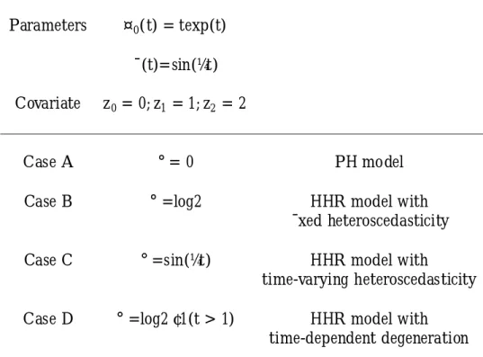
The rationale of using model (4) rather than (1) is twofold: (i) you add the heteroscedasticity exp(°0X); and (ii) the heteroscedasticity parameter °may also be time varying: ° = °(t). Table 1 summarizes several characteristics of the speci¯ed model.
[Table 1 about here.]
Throughout these examples, X = Z, and Z only takes three values: z0= 0; z1= 1; and z2 = 2;
the baseline ¤0(t) = texp(t) is used, and ¤0(t) =
Rt
0¸0(u)du. To illustrate the possibility of a
varying- coe±cient PH model being capable of treating the crossing hazards phenomenon, i.e., a special case of 'nonproportionality', we choose ¯(t) =sin(¼t). Case A assumes the varying-coe±cient PH model since ° = 0; Case B and Case C assume the HHR model with ¯xed and time-varying heteroscedasticities, respectively, when ° =log2 and °=sin(¼t). The time interval is selected to be (0; 2) for all cases.
[Figures 1(a)»1(d) about here.]
In Figures 1(a) to 1(c), three curves of logf¸(t; zj)=¸(t; zi)g are plotted, with the (j; i) pairs
equal (1,0), (2,1), or (2,0). In Fig. 1(a), however, only two curves are identi¯ed due to the fact that z2¡ z1 = z1¡ z0= 1. This can be called a case of degeneration, which results from
the model formulation of the 'proportional hazards'. That means, if the covariate values zi, zj,
and zk are representatives of some strata with zj ¡ zi = zk¡ zj, the homogeneity property of
the PH model makes two of the curves logf¸(t; zj)=¸(t; zi)g and logf¸(t; zk)=¸(t; zj)g coincide
or become very close in the LRR plot. Moreover, the observed curves retain the same 'shape' as ¯(t) except for being multiplied by the di®erence of zj ¡ zi. The situation di®ers in the
HHR model. In Figures 1(b) and 1(c), degeneration is not present, and the relative magnitudes among curves both change in time and are diverse between di®erent (j; i) pairs. In both ¯gures, if the two curves are close at some time, they may be separated some other 'place' (or 'time'). We can say that the existent heterogeneity assures a situation of no degeneration. But it is worth mentioning that if the heteroscedasticity parameter, °, is small or not very signi¯cant, degeneration may also take place in the LRR plot. In contrast to Case B, consider an example of time-dependent degeneration such as Case D: °=log2¢1(t > 1), where 1(¢) is the
indicator function; the other conditions are the same as those of Case B. Case D is designed to illustrate a special case of time-varying heteroscedasticity. The corresponding LRR plot is shown in Fig. 1(d), in which a dramatic change occurs at t = 1. When t · 1, ° = 0, the phenomena of degeneration and homogeneity observed in Figure 1(a) remain. When t > 1, °=log2, the curves are the same in Fig. 1(b). As a summary, nonproportionality accompanied by 'degeneration' implies that the nonproportionality can be modeled by the conventional PH model with a varying coe±cient, ¯ = ¯(t); otherwise the nonproportionality should be thought of as a phenomenon of heteroscedasticity which results from the variable 'age' and involves the parameter ° in model (4). Furthermore, if degeneration exists at several places but not everywhere, a time-varying coe±cient °(t) is possible. This means that at the place where there is degeneration, ^° does not signi¯cantly di®er from 0; elsewhere, however, ^° is signi¯cant and the heteroscedasticity parameter causes the interrelation among the curves to di®er.
3
Estimating Equations and the Sieve Method
Suppose there are n ordered, randomly right-censored observations (survival times or censored times) T1,T2, : : :, Tn. Let hi(t; Z; X ) and Ni(t) be the intensity process and counting process
for the ith individual and Yi(t) be the associated at-risk indicator at time t. Further denote
S1(t) = (1=n) n X i=1 Yi(t)exp(¯0Zi)¾if¤0(t)g¾i¡1; SZ(t) = (1=n) n X i=1 Yi(t)Zi(t)exp(¯0Zi)¾if¤0(t)g¾i¡1; and SV(t) = (1=n) n X i=1 Yi(t)Vi(t)exp(¯0Zi)¾if¤0(t)g¾i¡1; (8)
with predictable time-dependent covariates Zi(t) and Xi(t). In (8), ¾i =exp(°0Xi), and Vi(t) =
Xi(t)[1+exp(°0Xi)logf¤0(t)g]. By Johansen's decomposition (Johansen, 1983), the full
likeli-hood process has the following form: à L(t; ¯; °; ¤0) = ¦ Z t 0 hi(u)dNi(u) S1(u) ¢¦ Z t
0 S1(u)¸0(u)dNi(u)¢expf¡
Z t
0 nS1(u)dug: (9)
The ¯rst factor of (9) is the partial likelihood process. The logarithm of the partial likelihood is lp(t; ¯; °; ¤0) = X logf Z t 0 hi(u)dNi(u) S1(u) g: (10)
When time-varying coe±cients are not considered, that is when ¯(t) = ¯ and °(t) = ° in (4), taking partial derivatives of lp with respect to ¯ and ° leads to the following estimating
equation processes: X Z t 0fZi¡ SZ S1gdNi (u) = 0; X Z t 0fVi¡ SV S1gdNi (u) = 0: (11)
Moreover, a Breslow-type estimating equation for the baseline cumulative hazard can be con-structed as: ¤0(t) = X Z t 0 dNi(u) P Yj(u)exp(¯0Zj + °0Xj)[¤0(u)]exp(°0Xj)¡1: (12)
With model (2), statistical inferences based on a modi¯ed partial likelihood, other than the previous estimating equations, are also studied in Bagdonavi·cius, Hafdi, and Nikulin (2002). Since the baseline ¤0(t) is not eliminated in (10), a sieve method (Geman and Hwang, 1982)
is used to approximate it. By dividing entire observation period [0; ¿] into m segments by 0 = ¿0; ¿1; ¿2; : : : ; ¿m= ¿, we have the following approximation of ¤0(t):
¤(m)0 (t) = Z t 0 m X 1 ®j1(¿j¡1< u· ¿j)du: (13)
Under the varying-coe±cient model (4), a similar approximation can be imposed on ¯(t) and °(t), along with a little amendment of the estimating equations.
3.1
Piecewise e®ect and average e®ect analyses
Instead of using smoothing techniques, when the sieve approximations are taken for ¯(t) and °(t), ¯(t)¼Pm
1 ¯j1(¿j¡1 < t · ¿j) and °(t)¼Pm1 °j1(¿j¡1 < t· ¿j), it is termed a 'piecewise
e®ect' analysis of model (4):
¸(m)(t; Z; X ) = ®jf¤(m)0 (t)g¾j¡1¾j¹j; ¿j¡ 1 < t · ¿j; (14)
where ¸(m)(¢) denotes the approximation of ¸(¢), ¾j =exp(°j0X), and ¹j =exp(¯j0Z). In terms
of the cumulative hazard, ¤(¢), model (14) has the following expression: ¤(m)(t; Z; X) = ¤(m)(¿j¡1; Z; X) + [f¤(m)0 (t)g¾j¡ f¤
(m)
0 (¿j¡1)g¾j]¹j; ¿j¡ 1 < t · ¿j; (15)
with ¤(m)(¿0; Z; X) = ¤(m)0 (¿0) = 0. The estimating equation for ¤0 remains the same, but
those for ¯j and °j become:
X Z ¿j ¿j¡ 1fZi¡ SZ(m) S1(m) gdNi(u) = 0; j = 1; 2; : : : ; m; and X Z ¿j ¿j¡ 1fV (m) i ¡ SV(m) S1(m)gdNi(u) = 0; j = 1; 2; : : : ; m; (16) where V(m)and SK(m)are the corresponding V and SK(for any K) with ¤(m)0 (t) in place of ¤0(t).
The parameters f^®jgm1 ;f ^¯jgm1; and f^°jgm1) are simultaneously solved from the corresponding
estimating equations.
As stated in Sec. 1, when the partition f¿jgm1 gets ¯ner, each segment (¿j¡1; ¿j] contains
smaller number of observations, and the ¯nal estimates of ¯j and °j often will be nonsigni¯cant,
There is, however, a compromise which lies between the analysis using model (4) without a varying coe±cient and the PE analysis. That is, a 'thus-far-average' analysis (hereafter referred to as an 'average-e®ect' (AE) analysis) can be considered when an average coe±cient, ¯j and °j,
is calculated at each ¿js. In this case, ¯(t) and °(t) are replaced by ¯j and °j, for t · ¿j. With
the same sieve approximation, the hazard function of the k-th segment (i.e., ¿k¡1 < t · ¿k,
k · j) is
¸(m)(tjt · ¿j; Z; X) = ®kf¤(m)0 (t)g ¾j¡1¾
j¹j; ¿k¡ 1 < t· ¿k; (17)
In terms of the cumulative hazard, the AE model is expressed as: ¤(m)(tjt · ¿j; Z; X) = Z t 0 f m X k=1 ®k1(¿k¡1< u · ¿k)gf¤0(m)(u)g¾j¡1¾j¹jdu: (18)
Estimation under model (17) can be accomplished by simply replacing the integration interval
Rt
0 in (11) and (12) (and thus (13)) by
R¿j
0 . In this paper, we claim that the AE analysis (17)
is simply the HHR model implemented at each time point ¿j, 2 · j · m. When j = m, it is
reduced to the ordinary HHR model without varying coe±cients. In the following section, the SHT data are analyzed by the PE and AE methods and compared to the result of using the conventional PH model with a varying coe±cient.
4
Data Analysis
4.1
Nonproportionality of the Stanford heart transplant data
Analyses of the SHT data (Miller and Halpern, 1982; Lin, Wei, and Ying, 1993) suggested that 'age' and its square (age2) are important explanatory variables. Since there is nonproportion-ality among di®erent age groups (see Fig. 2 below), inclusion of the covariate age2is to explain
the crossing-e®ect. See also Aitkin, Laird, and Francis (1983) and Arjas (1986, 1988) for more discussion. To deal with the nonproportionality, Marzec and Marzec (1997) ¯tted the PH model with a varying coe±cient on the parsimony of only one covariate, age, and proposed goodness-of-¯t tests to demonstrate the validity of their sieve-approximated varying-coe±cient setting. The SHT data analyzed in Marzec and Marzec (1997) contain 154 observations (denoted by T1 · T2· : : : · T154), of which 102 are noncensored failures. To motivate the accommodation
of a heteroscedasticity component by using the HHR model, on the other hand, survivor func-tions according to di®erent age groups can be displayed. First, the 154 patients are divided into four groups according to the three quartiles of age: 35.25, 44.5, and 49.0. Each group contains 38 or 39 patients. Since there is no signi¯cant di®erence between the younger two groups (lo-grank statistic=0.0050, p-value=0.9436), we combine them into a single group and denote the patients with age< 45, 45 ·age·49, and age¸50 as groups 1, 2, and 3, respectively. Instead of showing the Kaplan-Meier (K-M) estimates directly, however, we mimic the idea behind the LRR plot in Sec. 2 and display the pairwise log-ratios logf^¤2(t)= ^¤1(t)g, logf^¤3(t)= ^¤2(t)g,
and logf ^¤3(t)= ^¤1(t)g, where ^¤j(t) =¡logf ^Sj(t)g; j = 1; 2; 3; and ^Sj(t) is the K-M estimate of
log-ratio is plotted at the union of the two sets of time points where K-M estimates have been calculated. Plotting the log-ratios, logf ^¤j(t)=^¤i(t)g, of all possible (j; i) pairs has the merit of
exploring pairwise relations among groups. Moreover, proportionality, hazards crossing, and time-varying e®ect may also be explored. If the proportional hazards rule holds, the ratios must be some constants, although small °uctuations are possible. Otherwise, nonconstancy may exist (which implies ¯ = ¯(t)). Moreover, if a curve crosses the horizon 'log-ratio=0' (the dotted line) at some t = t0, it means that there is a hazards crossing near t0 between the two
associated age groups.
[Figure 2 about here.]
In Fig. 2, the curves show nonproportionality among groups. Moreover, since the interrelations of the three curves change in time, heteroscedasticity may also exist. The existence of time-varying heteroscedasticity will be shown later by the LRR plot. The estimated cumulative hazards of groups 1 and 2, ^¤1and ^¤2, cross each other ¯rst at a time of between 130 and 250
days, and second at a time of 2127 days. The curve logf ^¤2=^¤1g is basically concave. Another
curve, logf ^¤3= ^¤1g, crosses the horizon 'log-ratio=0' before 25 days and has a similar shape.
However, the two curves have di®erent curvature (in terms of t) which results in a third plot, logf^¤3=^¤2g, distinct from the former two. As a whole, the three curves give the impression
that the three groups are heteroscedastic, in particular at a time between 200 and 700 days which corresponds to the third segment in the following PE analysis and LRR plot.
4.2
Piecewise e®ect (PE) analysis and LRR plot
When the HHR model is used, the number of segments, m, for the sieve approximation has to be decided. Since Hsieh (2001) suggested m to be of the order O(n1=3) to make the asymptotic
results valid, we divide the observation period [0,2984] into m = 5 segments, each containing 30 or 31 observations, failured or censored. In the setting of PE analysis, the parameters are allowed to di®er between segments. For the SHT data, the ¹- and ¾- components of the PE model are:
¹j = exp(¯1jage + ¯2jage2); and
¾j = exp(°jage); ¿j¡ 1 < t · ¿j; j = 1; 2; : : : ; 5: (19)
In contrast, Marzec and Marzec's (1997) analysis is basically the varying-coe±cient PH model without the covariate age2. Thus, their model can be treated as being nested in the current PE model, via which the needs to add age2 and impose the ¾-component can be tested by the signi¯cance of ^¯2j and ^°j. In particular, bias of the e®ect estimate of age can be avoided because
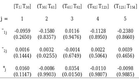
in model (19), heterogeneity has been accounted for by the ¾-component. Table 2 shows the estimated values of all parameters ¯1j, ¯2j, and °j which vary from segment to segment, showing
the time-dependent 'e®ect' from the model considered. Among those estimated values of °j, in
particular, ^°3 (=0.0354) signi¯cantly di®ers from zero (p-value=0.015); the estimate ^°1 has a
can increase when additional sample is accumulated; that is, when the analysis is extended to the next segment using the following AE method.
When an HHR model has been estimated through the PE analysis, logarithm of the es-timated relative risk (LRR) can only be plotted according to several predisposed covariate values. In Fig. 3, LRR plot of three combinations, logf^¸(t; z1)=^¸(t; z0)g, logf^¸(t; z2)=^¸(t; z1)g,
and logf^¸(t; z2)=^¸(t; z0)g are presented for age= 35 (z0), 45 (z1), and 55 (z2), respectively.
These values are representative of the three age groups discussed previously and retains the property, z1¡ z0 = z2¡ z1, to make a degeneration possible if the underlying model is an
homogeneous one (i.e., the PH model with or without a varying coe±cient). The curves in Fig. 3 look like (but are not) step functions due to the sieve approximation. In the third segment (i.e., the time interval of [227; 631] days), the three curves are very distinct. In the ¯rst segment (i.e., the time interval of (0; 50] days), logf^¸(t; z1)=^¸(t; z0)g and logf^¸(t; z2)=^¸(t; z1)g are closer
to, but still can be distinguished from each other (this can be observed more clearly when the plot is ampli¯ed). As for the remaining segments, degeneration becomes clear and heteroscedas-ticity may disappear. In conclusion, the SHT data appears to be an example of time-dependent degeneration illustrated by the last example in Sec. 2., implying a varying-coe±cient °(t).
In practice, one may ask the question: When the true model is the PH model and the HHR model is adopted, will the LRR plot exhibit non-degeneration? The answer relies on the large sample asymptotics of the parameter estimates. For simplicity, let X = Z and dim(Z) = 1. The statistics ( ^¯¡ ¯; ^°¡ °)0 and ^¤0(t)¡ ¤0(t) obtained from the OEE method (Hsieh, 2001;
Theorem 1) have the order of Op(1=pn). According to (7), the estimated log-relative risk
between strata Zj and Zi is
logRR =d expf^°(zj ¡ zi)g ¢logf^¤0(t)g + ( ^¯+ ^°)(zj ¡ zi)
= Op(1=pn) + ^¯(zj¡ zi); for 0 < t < 1; (20)
which retains the shape of ¯(¢) for an large sample size, if the true model is the PH model (° = 0 or °(t) = 0) and 0 < ¤0(t) <1 for 0 < t < 1. When sample size is small, the LRR
plot speci¯c to the HHR model may not be 'stable', in particular at the early stage of time. [Table 2 and Figure 3 about here.]
4.3
Average e®ect (AE) analysis
A di®erent perspective results in model (17) or (18) when an average e®ect is of interest even if the e®ect is time-varying, whereas investigations are made along the time axis so that the information about the model and parameters are collected as a process. Speci¯cally, let the estimation be executed at the time points ¿1; ¿2; : : : ; ¿5. In this case, a thus-far-average estimate
is calculated at each ¿j, and this estimate has a dynamic meaning with regards to progressing
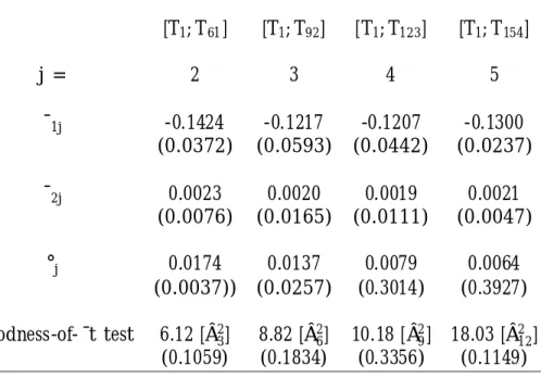
time. It has the interpretation of an ageing e®ect at the population level. The results of the AE analysis are displayed in Table 3. (The analysis at ¿1is exactly the result of the ¯rst segment
[Table 3 about here.]
In summary, the di®erence between the PE and AE analyses is that the PE model is actually an approximation of the varying-coe±cient model (4), and it assumes that for each time segment, the coe±cients may di®er. On the other hand, the AE model is not an approximation of (4). It is simply a practice of the HHR model at the selected times ¿1 to ¿m. For the
goodness-of-¯t test for model validity in Table 3, see Hsieh (2001) and Wu, Hsieh, and Chen (2002) for further details. In brief, it is an omnibus test for global adequacy of ¯tting the HHR model at t = ¿j; j = 2; 3; : : : ; 5, and the constructed testing statistic follows, asymptotically, a chi-square
distribution with 3(j¡ 1) degrees of freedom for 2 · j · 5. From the last panel of Table 3, the results of the goodness-of-¯t test show that the HHR model with AE analysis is adequate for t = ¿j; j = 2; 3; : : : ; 5.
4.4
Implication of the results
In terms of the partitions taken for the sieve approximation, there is no segment-to-segment correspondence between the previous analyses and those of Marzec and Marzec (1997). Never-theless, comparisons can be made by carefully connecting the results of the LRR plot in Fig. 3 and Tables 2 and 3. In our PE analysis, although most of the estimates ( ^¯1j; ^¯2j; ^°j; j = 1; : : : ; 5)
are not signi¯cant, PE analysis is still necessary as the ¯rst step to investigate the existence of the varying coe±cients. From Table 2, the signi¯cance levels of ^°1 (p-value of 0.115) and
^
°3 (p-value of 0.015) imply that heteroscedasticity exists in the corresponding periods. The
LRR plot displayed in Fig. 3 gives a similar explanation. Since the information used in the PE analysis is accumulated, nonsigni¯cant results appearing in the PE analysis may become signi¯cant in the AE analysis. The goodness-of-¯t tests for model adequacy in Table 3 reveal that the HHR model is adequate.
As compared with the ¯rst analysis (a partition with equal time intervals) of Marzec and Marzec (1997), their ¯rst segment, [0,746] days, contains 98 observations, nearly corresponding to the [T1; T92] interval of our AE analysis in Table 3. However, it should be noted that if a
varying-coe±cient PH model without heteroscedasticity and which omits the covariate, age2, can take care of the nonproportionality, the LRR plots in Fig. 3 should not have this pattern. Degeneration may exist everywhere. In addition, ^¯23 and ^°3in the AE analysis should be both
nonsigni¯cant since the varying-coe±cient PH model can be viewed as a submodel nested in the more-extended varying-coe±cient HHR model. From Table 3, since both ^¯23 and ^°3 are
signi¯cant (p-values of 0.017 and 0.026) at the level of 0.05, Marzec and Marzec's estimate in this period is a biased one. Under model (4) and its variants (14) and (17), the result of Marzec and Marzec can be reasonably explained by that the in°uences of omitting the heteroscedasticity and the covariate age2 cancelling each other. Similarly, in our AE analysis (Table 3), ^°
5 is
nonsigni¯cant in [T1; T154], which corresponds to the result of a conventional PH analysis with
the covariates of age and age2. Finally, although the estimated heteroscedasticity parameter may not be signi¯cant in the AE analysis, the heteroscedasticity component ¾ =exp(° age) should not be dropped from the analysis due to the fact that, from Fig. 2 and Fig. 3, the
heterogeneity is from the covariate 'age'. This is similar to the concern of 'variable selection' procedures in an ordinary linear regression where variables of interest should always be included. Importantly, with a nonsigni¯cant ¾-component, ¯ts can be improved over those without it.
5
Discussion
To deal with nonproportional hazards, heterogeneity due to variation over subjects is the main focus of the current study. To diagnose heterogeneity, survival data can be grouped according to some important variable (for example, 'age' as in the SHT data). By plotting log-ratio of estimated cumulative hazards of all pairs based on the K-M survivor estimates, ¯rstly, interre-lation among age groups can be explored (Fig. 2). If the K-M estimates cross one another at an early stage and the interrelation changes in time, heterogeneity may exist, and incorporation of heteroscedasticity in a Cox-type regression can be taken into consideration. The method of ¯tting the varying-coe±cient PH model to tackle nonproportional hazards phenomena is only feasible when there is no heteroscedasticity. In this paper, we demonstrate that when the non-proportionality is a result of heterogeneity, the varying-coe±cient HHR model (4) is applicable. After applying model (4), an LRR plot (Fig. 3) is suggested to diagnose the need of imposing ¯(t) and °(t). Constancy of log-ratios of relative risk and degeneration of some curve(s) are used as criteria. In our analyses of the SHT data, the estimated piecewise parameters di®er at various time intervals (the PE model). As well, the average estimates of the three parameters change in a pointwise manner at ¿s (the AE model). From Table 3, ^°s decrease in ¿j. This
also implies that there is time-dependent heteroscedasticity when age is the only covariate of concern.
The existent heteroscedasticity may be easily neglected if the varying-coe±cient PH model (1) is used. In Table 3, the AE analysis made at ¿5 (that is, the column [T1; T154]) has a
nonsigni¯cant estimate of °: ^° = 0:0064 with a p-value of 0.39. This corresponds to the conventional analysis using the PH model in which age and age2 are considered explanatory
variables. The inclusion of age2 reveals that there is nonproportionality. In the analysis of
Marzec and Marzec, the nonproportionality is accounted for by ¯(t) in model (1) where 'age' is the unique explanatory variable. In this paper, however, we demonstrate by the LRR plot of Fig. 3 that there is heterogeneity which can be adequately modeled by a time-dependent heteroscedasticity parameter: °(t). For diagnosing °(t), we suggest using 'degeneration' as a tool for visualization. Moreover, time-dependent degeneration implies time-dependent het-eroscedasticity, but not vice versa. In the case when °is not very large, a practitioner need only be concerned with the signi¯cance of ^° and its time-varying properties, while degeneration is a valid criterion of the varying coe±cient °(t). As the heteroscedasticity parameter ° becomes large, a formal test for its time-varying property along with a companion diagnostic tool still needs to be developed.
In fact, the HHR model is a special case of a transformation model with heteroscedastic error terms (Hsieh, 1995). In this article, we emphasize that adequate modeling of the existent heteroscedasticity can, in some cases, explain the time-varying e®ect. In addition, coe±cients
in the HHR model can also be time dependent. In that case, one has to pay attention to the rationale of using a varying-coe±cient setting. If the dynamics of the condition implied by the covariate process or data history can in°uence the e®ect and signi¯cance of the covariate itself, a varying-coe±cient model is reasonable. In an analysis of follow-up experimental data, 'dynamical' meaning can implicitly be designed into the study. For observational data, on the other hand, conclusions about the e®ects of environmental factors on changes in the health condition or behavior should be drawn carefully.
References
M. Aitkin, N. Laird, and B. Francis, "A reanalysis of the Stanford heart transplant data (with discussion)," Journal of the American Statistical Association vol. 78 pp. 264-292, 1983. E. Arjas, "Stanford heart transplantation data revisited: a real-time approach," Modern
Sta-tistical Methods in Chronic Disease Epidemiology (edited by S.H. Moolgavkar and R.L. Prentice) pp. 65-81, John-Wiley: New York, 1986.
E. Arjas, "A graphical method for assessing goodness of ¯t in Cox's proportional hazards model," Journal of the American Statistical Association vol. 83 pp. 204-212, 1988. V. Bagdonavi·cius, M. A. Hafdi, and M. Nikulin, "The generalized proportional hazards model
and its application for statistical analysis of the Hsieh model," Proceeding of the France-Japonise Conference, Chamonixe, France, 2002.
D. R. Cox, "Regression models and life-tables (with discussion)," Journal of the Royal Statis-tical Society, Series B vol. 34 pp. 187-220, 1972.
S. Geman and C.-R. Hwang, "Nonparametric maximum likelihood estimation by the method of sieves," The Annals of Statistics vol. 10 pp. 401-414, 1982.
F. Hsieh, "The empirical process approach for semiparametric two-sample models with het-erogeneous treatment e®ect," Journal of the Royal Statistical Society, Series B vol. 57 pp. 735-748, 1995.
F. Hsieh, "On heteroscedastic hazards regression models: theory and application," Journal of the Royal Statistical Society, Series B vol. 63 pp.63-79, 2001.
S. Johansen, "An extension of Cox's regression model," International Statistical Review vol. 51 pp. 165-174, 1983.
D. Lin, L. J. Wei, and Z. Ying, "Checking the Cox model with cumulative sums of martingale residules," Biometrika 80, pp. 557-572, 1993.
T. Martinussen, T. H. Scheike, and I. M. Skovgaard, "E±cient estimation of ¯xed and time-varying covariate e®ects in multiplicative intensity models," Scandinavian Journal of Statistics 29, pp. 58-74, 2001.
L. Marzec and P. Marzec, "On ¯tting Cox's regression model with time-dependent coe±-cients," Biometrika 84, pp. 901-908, 1997.
R. Miller and J. Halpern, "Regression with censored data," Biometrika 69, pp. 521-531, 1982. L. S. A. Murphy and P. K. Sen, "Time-dependent coe±cients in a Cox-type regression model,"
J. O'Quigley, "On a two-sided test for crossing hazards," The Statistician vol. 43 pp. 563-569, 1994.
C. Quantin, T. Moreau, B. Asselain, T. Maccario, and J. Lellouch, "A regression survival model for testing the proportional hazards hypothesis," Biometrics vol. 52 pp. 874-885, 1996.
D. M. Stablein, and I. A. Koutrouvelis, "A two-sample test sensitive to crossing hazards in uncensored and singly censored data," Biometrics vol. 41 pp. 643-652, 1985.
H.-D I. Wu, F. Hsieh, and C.-H. Chen, " Validation of a heteroscedastic hazards regression model," Lifetime Data Analysis vol 8 pp. 21-34, 2002.
Table 1: Speci¯ed conditions for the varying-coe±cient PH and HHR models. A general formula of the assumed model is: ¸(t; Z; X) = ¸0(t)f¤0(t)gexpf°(t)Zg¡1expf¯(t) + °(t)gZ, in
which we choose X and Z to be identical. Case A assumes a varying-coe±cient PH model. Cases B and C assume HHR models with ¯xed and time-varying heteroscedasticities, respectively. Case D speci¯es an HHR model with dependent degeneration, a special case of time-varying heteroscedasticity.
Parameters ¤0(t) = texp(t)
¯(t)=sin(¼t) Covariate z0= 0; z1= 1; z2 = 2
Case A °= 0 PH model
Case B ° =log2 HHR model with ¯xed heteroscedasticity Case C °=sin(¼t) HHR model with
time-varying heteroscedasticity Case D ° =log2¢1(t > 1) HHR model with
Table 2: Analyses of SHT data using the piecewise e®ect method calculated at t = ¿j
(meaning ¿1 = T30; ¿2 = T61; : : : ; ¿5 = T154.) Values in parentheses are the p-values of the
associated Wald tests for signi¯cance.
[T1; T30] (T30; T61] (T61; T92] (T92; T123] (T123; T154] j = 1 2 3 4 5 ¯1j -0.0959 -0.1580 0.0116 -0.1128 -0.2380 (0.2650) (0.8357) (0.9476) (0.8950) (0.8660) ¯2j 0.0016 0.0032 -0.0014 0.0022 0.0039 (0.1444) (0.0255) (0.6749) (0.5064) (0.4656) °j 0.0160 -0.0086 0.0354 -0.0110 -0.0098 (0.1147) (0.9903) (0.0150) (0.9807) (0.9885)
Table 3: Analyses of SHT data using the average e®ect method calculated at t = ¿j; j =
2; 3; 4; 5. Values in parentheses are the p-values of the associated tests for signi¯cance of pa-rameters or the model. For j = 1, the AE analysis is exactly the PE analysis in Table 2, so it is omitted from this table. The last panel shows the goodness-of-¯t test for model validity.
[T1; T61] [T1; T92] [T1; T123] [T1; T154] j = 2 3 4 5 ¯1j -0.1424 -0.1217 -0.1207 -0.1300 (0.0372) (0.0593) (0.0442) (0.0237) ¯2j 0.0023 0.0020 0.0019 0.0021 (0.0076) (0.0165) (0.0111) (0.0047) °j 0.0174 0.0137 0.0079 0.0064 (0.0037)) (0.0257) (0.3014) (0.3927) Goodness-of-¯t test 6.12 [Â2 3] 8.82 [Â26] 10.18 [Â29] 18.03 [Â212] (0.1059) (0.1834) (0.3356) (0.1149)