2
nPattern Run-Length for Test Data Compression
Cheng-Ho Chang, Lung-Jen Lee, Wang-Dauh Tseng and Rung-Bin Lin
Department of Computer Science & Engineering Yuan Ze University
Taoyuan, Taiwan s976145@mail.yzu.edu.tw
Abstract- This paper presents a pattern run-length compression method. Compression is conducted by encoding 2|n|
runs of compatible or inversely compatible patterns into codewords in both views either inside a single segment or across multiple segments. With the provision of high compression flexibility, this method can achieve significant compression. Experimental results for the large ISCAS’89 benchmark circuits have demonstrated that the proposed approach can achieve up to 67.64% of average compression ratio.
Keywords- automated test equipment (ATE); pattern run-length; circuit under test (CUT); test data compression.
I. INTRODUCTION
AS the increased complexity of System-on-a-Chip (SOC),
more functions and hence more transistors have been crammed into a single chip. Although producing robust designs, much more faults are created accordingly. To detect them, a large amount of test data with longer testing time is essentially required, which has majorly increased the cost of manufacturing testing for integrated circuits [1]-[4]. An actively researched area is to use the compression techniques to reduce the large test data volume so as to extend the life of the aged testers that have limited memory.
Test data compression can reduce the large test data volume transmitted to the circuit under test (CUT) where, typically, only a small portion of test data is care bits. During compression, the large portion of don’t cares can be flexibly specified to promote compression effect without impacting the fault coverage. In addition to saving in ATE memory, it saves a significant amount of testing time. During test, the compressed data is first sent to CUT, decompressed losslessly by the on-chip decoder and then serially scanned into the scan chain for later test. Techniques of test data compression can broadly be classified into three types: Code-based schemes,
Linear-decompression-based schemes, and Broadcast-scan-based schemes [5]. Code-based scheme transfers test data into a number of codewords by recognizing specific properties embedded in corresponding bit-strings of the test data. The Huffman code [6] provides the shortest average codeword length among all uniquely decodable variable length codes. Although optimal in statistical code, it
suffers from its exponentially grown decoder size. The extending works such as Huffman coding-based SHC [7], OSHC [8] and VIHC [9] are also proposed. Selective Huffman Coding [7] is an efficient test data compression method with low hardware overhead, which merely encodes the most frequently occurring symbols. Variable-Length Input Huffman Coding [9] analyzes the compression environment and fully exploits the type and length of pattern during compression. A 9C technique [10] uses exactly nine codewords to compress the pre-computed data of intellectual property cores in SOC. It is flexible in utilizing both fixed- and variable-length blocks. Besides, run-length-based compression method is also an effective code-based compression scheme, which encodes runs of repeated values. Examples include GOLOMB [11], FDR [12], ALT-FDR [13], PRL [14], and EFDR [15]. ALT-FDR [13] is a variable-to- variable length compression method adopting the same encoding manner as FDR [12]. PRL [14] is also efficient in compressing consecutive patterns. BM [16], a block merging technique in which good compression effect was achieved by encoding runs of fixed-length blocks, only the merged block and number of block merged are recorded. The RL-HC [17] combines the above two methods: run-length-based and Huffman coding for scan testing to reduce test data volume, test application time, and scan in power. MD-PRC [18], a multi- dimensional pattern run-length compression method was recently proposed where multiple pattern information is considered for compressing runs of variable-length patterns.
In this paper, we present the 2n Pattern Run-Length (2n-PRL) compression method. The basic idea is to iteratively encode 2|n| runs of (inversely) compatible patterns either inside a single segment or across multiple segments into codewords. Being flexible, this method can achieve significant compression. The decompression logic is also simple and easy to implement. Experimental results have demonstrated its efficiency in compression. The rest of this paper is organized as follows: Section II presents the proposed method and the decompression architecture. To evaluate the effectiveness of the proposed method, in Section III, experiments for six large ISCAS’89 benchmark circuits
562
are performed. Finally, we conclude this work in Section IV. II. PROPOSED METHOD
A. Test Data Compression
Two patterns are recognized as compatible if every bit pair at the same position has the same value or any of them is a don’t-care. In the proposed approach, test set is first partitioned into several fixed-length (L-bit) segments in which L is a power of 2. Compression is then conducted on 2|n| compatible patterns where n is a signed integer. Depending on the encoded pattern, the proposed method can be classified into two types: the internal 2n-PRL (n < 0) and the external 2n-PRL (n ≥ 0), characterized by the sign of the exponent n. The internal 2n-PRL is conducted inside a single segment for compressing 2|n| runs of compatible sub-segments. For example, consider the segment “100011011011” with length of 12 bits. If it is divided into 4 sub-segments with length 12 × 2-2 = 3 bits for each, data in the last 3 sub-segments will be found inversely compatible with the first sub-segment. In this case, the segment can be encoded by -2-2-PRL, where the negative sign in front of the radix represents an inverse compatibility of the rest sub-segments with the first sub-segment, and the exponent value -2 represents that this segment is divided into 1/2-2 = 4 segments. To represent the encoding of -2-2-PRL, we show the internal 2n-PRL codeword format with 3 components in Fig. 1(a), where sign (S) is the sign in front of the radix (“1” for negative and “0” for positive), exponent (E) is the value in the exponent field (including the sign of the exponent), and
pattern (P) is the first sub-segment data with its don’t-cares
properly filled-in to match the compatibility with all other sub-segments. As a result, this segment can be encoded into the codeword 1 110 100 as shown in Fig.1 (b). Note that, a 3-bit exponent field is assumed in this case and we use a 2’s complement-like format to represent the value in the exponent field which will be explainedlater.
Alternatively, the external 2n-PRL is conducted on 2n consecutive compatible segments. For example, if two consecutive segments, Si = “001xx0000xx0” and Si+1 =
sign 1 bit exponent pattern L/2nbits K bits (a) 100 011 011 011 Single segment -2-2-PRL 1 110 100 E S P (b)
Figure 1. (a) Codeword format for internal 2n-PRL (b) an encoding example. sign 1 bit exponent K bits (a) 001000000000 001xx0000xx0 00xx00000000 +21-PRL 0 001 E S Sbase Si Si+1 (b)
Figure 2. (a) Codeword format for external 2n-PRL (b) an encoding example.
“00xx00000000”, to be encoded are compatible with the base segment, Sbase = “001000000000”, which is the previous
segment remained in the buffer in the decompressor.These two segments can be encoded by +21-PRL, where the plus sign in front of the radix represents that the base segment are compatible (not inversely compatible) with the successive segments and the exponent value 1 represents that there are 21 = 2 consecutive segments compatible (or inverse compatible) with the base segment. To represent the encoding of +21-PRL, the external 2n-PRL codeword format with 2 components is shown in Fig. 2(a). The meanings of the two components in the codeword for the external 2n-PRL are the same with those in the internal 2n-PRL. As a result, the above segments can then be encoded as 0 001 as shown in Fig. 2(b). Typically, the external type of encodings is used when there is a valid base segment in the buffer (i.e., there exists at least one succeeding segment compatible with the base segment). While the internal type of encodings is used to either fill-in the buffer in the beginning or to renew the buffer when the base segment is invalid.
In the following, as shown in Fig. 3, a simple example with a simplified test set is introduced to illustrate the proposed
11X11XX111XXXXX1X1XXXXX10XXXXX0X X0XXXXXXX01XXXXXX10XXXX10XXXXXXX XXXXXXXXX1XXXXX1X0X010XX1XXX1XXX 100XXXX1101XXXX0
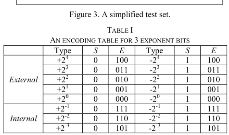
Figure 3. A simplified test set. TABLE I
AN ENCODING TABLE FOR 3 EXPONENT BITS
Type S E Type S E External +24 0 100 -24 1 100 +23 0 011 -23 1 011 +22 0 010 -22 1 010 +21 0 001 -21 1 001 +20 0 000 -20 1 000 Internal +2 -1 0 111 -2-1 1 111 +2-2 0 110 -2-2 1 110 +2-3 0 101 -2-3 1 101 compression method. In this example, test data is divided into ten 8-bit segments and the exponent length is assumed 3 bits. Table I shows the encoding table where a 3-bit exponentare used for 16 encodings ranged from ±24-PRL to ±2-3-PRL. As
can be seen, the encoding for the exponent field is very similar to the 2’s complement representations except that the most negative binary number 100 is moved to represent the biggest positive number +4 rather than -4. For an n-bit binary, the 2’s complement representations can offer an encoding ranged from -2n-1 to +2n-1 – 1, while in the proposed representation,
the encoding is ranged from - (2n-1 – 1) to +2n-1. Table II shows the compression results, where the column “Buffer” shows the base segment in the buffer after the decompression of codeword. Initially, the buffer is empty and hence the internal 2n-PRL is used to fill in S
1 to be the base segment.
Since a larger absolute value of exponent can achieve a better TABLE II
A SIMPLE ENCODING EXAMPLE FOR L=8
Segments Buffer Codewords Types S1 11X11XX1 11111111 01011 +2-3-PRL S2 11XXXXX1 11111111 0001 +21-PRL S3 X1XXXXX1 S4 0XXXXX0X 00000000 1001 -21- PRL S5 X0XXXXXX S6 X01XXXXX 10101010 011010 +2-2-PRL S7 X10XXXX1 01010101 1010 -22-PRL S8 0XXXXXXX S9 XXXXXXX S10 X1XXXXX1
compression, during the fill-in of S1, the encoding types of
±2-3-PRL are firstly considered. By partitioning S1 into 23
sub-segments with 1 bit for each, the first sub-segment is
Start
Set exponent field length = K Set i = 2K-1 & j = 2K-1– 1 i ≥ 0? Encode segments by +2i-PRL i ≥ 0? Yes Segments encodable by +2i-PRL? Yes Segments encodable by -2i-PRL? Encode segments by -2i-PRL Yes No Any segments left?
Yes i = i – 1 No Segment encodable by +2-j-PRL? Yes Encode segment by +2-j-PRL Yes Segment encodable by -2-j-PRL? Encode segment by -2-j-PRL Yes No j ≥ 1? Yes No j = j – 1 No No End No
Exception and input original segment
D0 D1 D2 D3 D4 D5 D6 D7
Decoder
Select HoldMUX MUX MUX MUX
Buffer
To scan chainCodeword from ATE
Input Inverse D0 D1 D2 D3 D4 D5 D6 D7
Decoder
Select HoldMUX MUX MUX MUX
Buffer
To scan chainCodeword from ATE
Input Inverse
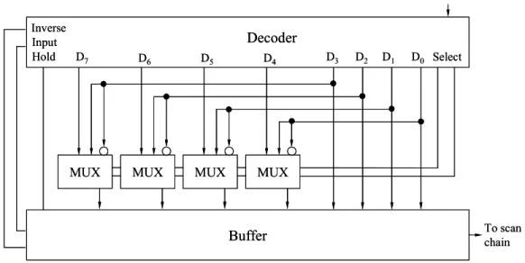
Figure 5. The decompression architecture with L = 8 and K = 2.
found compatible with all the rest sub-segments.
Consequently, S1 is encoded by +2-3-PRL with the
codeword 0 101 1. After decompression, the base segment (Sbase) in the buffer becomes “11111111”. Next, segments S2
and S3 are found compatible with Sbase, they can be
compressed by +21-PRL. Similarly, the segments S
4 and S5
are inversely compatible with Sbase, they are compressed by
-21-PRL. S
6 is not compatible or inversely compatible with
Sbase (i.e., Sbase is invalid and has to be renewed). As can be
seen, S6 can be compressed through the encoding of +2-2-PRL by partitioning it into 4 sub-segments with “10” as the encoded pattern and, after decompression, Sbase is updated as
10101010.
Now, the segments from S7 to S10 can be compressed by
-22-PRL and S
base is inverted to 01010101. Consequently,
total test data volume is reduced from the original 80 bits to 23 bits with the compression ratio of 71.25%. Inevitably, if some segments are found not fit any of the 2n-PRL encoding types, to cover these uncompressible segments, the least frequently-used type will be removed and the associated control code (sign + exponent) will be designated as “exceptions”. The exception type will be compressed by the codeword format constituted by a control code followed by the entire segment data. Fig. 4 shows the complete encoding flow for the proposed method.
MUX
Original
2
-1-2
-1Output
Selection
Figure 6. The multiplexer for 2-bit exponent.
B. The Decompression Architecture
In this section, we introduce the decompression architecture. As shown in Fig. 5, the decompression architecture is designed for the compression of test data with segment length equal to 8 (L = 8) and the exponent length equal to 2 (K = 2). The encoding range is from ±22-PRL to ±2-1-PRL. The main components include a decoder, a multiplexer array, and an 8-bit buffer. Decompression starts by receiving and identifying the control bits from the ATE. The corresponding signals are then launched by the decoder. For the internal 2n-PRL decompression, the buffer will be filled-in through a proper broadcast of the encoded pattern depending on the compression type. For the decompression of external 2n-PRL, the base segment in the buffer can be inverted, updated or remains unchanged according to the associated signals. We will explain the function for each component as follows.
Decoder: It is a Finite State Machine (FSM), which
receives codewords from ATE, decides the next state and launches the associated signals to the multiplexer array and buffer. Three signals, “Inverse”, “Input” and “Hold” decide the buffer content to be “inverted”, “updated” or “unchanged” respectively. 0.42 0.45 0.48 0.51 0.54 0.57 2 3 4 Exponent Length (K) Co m pr e ss io n Ra tio
Figure 7. The impact of different K’s on compression effect for circuit s5378
inverters. As shown in Fig. 6, the multiplexers are placed in between the decoder and the buffer, each of which determines the output data according to the selection signal from the decoder. Fig. 6 shows the multiplexer. If the selection signal is “00” (i.e., -2-1-PRL), the attached 4-bit encoded pattern and its inversion pattern are output. If the selection signal is “01” (i.e., +2-1-PRL), a direct broadcast of the attached 4-bit encoded pattern is output. If the selection signal is “10”, the original 8-bit segment data is directly output.
Buffer: It receives the decompressed test data and sends
them to the scan chain for later test. The data in buffer is also treated as the base segment for the follow-up encoding.
III. EXPERIMENTAL RESULTS
We have implemented experiments on six large ISCAS89 benchmark circuits adopting test data generated by Mintest [19] ATPG with dynamic compaction. The compression effect is evaluated by the compression ratio, which is defined as CR% = [(|TD| - |TE|) / |TD|] × 100%, where |TD| is the size of
test set and |TE| is the size of the compressed test set.
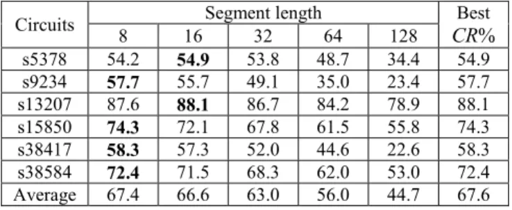
At first, we explore the impact of varying K’s (length of exponent) on the compression effect on the circuit s5378. As shown in Fig. 7, the compression ratio increases with the increase in K. It reaches the peak at K = 3 and then decreases as K continues to grow. For the compression adopting a smaller K, due to fewer matches in compression types, only low compression is obtained. While for those adopting larger K’s, compression effect is negatively affected by the long exponent in each codeword. Exploration on the optimal segment length (L) under a certain K is also conducted on the circuit s5378. The resulting compression ratios are presented in Fig. 8, where continue the above experiment, K is assumed 3 and L varies from 8 to 128. As shown, the best compression ratio occurs at L = 16. In Table III, we explore the impact of L on compression effect for the six circuits with the best ones bolded and reports the best results in the last column. As shown, four out of the six reach the best compression ratios at L = 8 while the other two at L = 16.
In the following, we analyze the hardware overhead of the decompressor architecture. The benchmark circuits and the decompressor were synthesized using Synopsys Design Compiler with a single scan chain. The decompressor area overhead is computed as follows:
Area overhead = areaofbenchmark circuit 100% or
decompress of
area
×
Table IV shows the comparison results for the proposed method with other methods for six large ISCAS89 benchmark circuits. As shown, the decompressor area overhead for the proposed method is reasonably small.
0.3 0.35 0.4 0.45 0.5 0.55 0.6 8 16 32 64 128
Segment Length (bits)
Co m pr es sio n Ra tio
Figure 8. The impact of different L’s on the compression effect for circuit s5378.
TABLE III
THE COMPRESSION EFFECT UNDER DIFFERENT L’S FOR SIX CIRCUITS Circuits 8 16 32 64 128 Segment length CR%Best
s5378 54.2 54.9 53.8 48.7 34.4 54.9 s9234 57.7 55.7 49.1 35.0 23.4 57.7 s13207 87.6 88.1 86.7 84.2 78.9 88.1 s15850 74.3 72.1 67.8 61.5 55.8 74.3 s38417 58.3 57.3 52.0 44.6 22.6 58.3 s38584 72.4 71.5 68.3 62.0 53.0 72.4 Average 67.4 66.6 63.0 56.0 44.7 67.6 TABLE IV
COMPARISONS WITH PREVIOUS WORKS IN DECOMPRESSOR AREA OVERHEAD(%)
Circuits GOLOMB [11] FDR [12] EFDR [15] SHC [7] VIHC [9] [10] 9C [16] BM 2n-PRL
s5378 4.0 7.8 8.3 16.0 5.8 8.2 12.8 4.6 s9234 3.2 5.9 6.3 13.0 4.6 6.2 9.7 3.6 s13207 4.1 3.5 3.7 5.7 2.2 3.7 5.8 1.7 s15850 2.0 3.6 3.8 6.5 2.3 3.8 5.9 1.8 s38417 0.5 1.4 1.5 2.0 0.7 1.5 2.3 0.6 s38584 0.7 1.5 1.6 2.0 0.7 1.6 2.5 0.6 Table V reports the compression ratios compared with other previous works such as GOLOMB [11], FDR [12], ALT-FDR [13], EFDR [15], Huffman coding-based SHC [7], VIHC [9], RL-HC [17], 9C [10], BM [16] and MD-PRC [18]. Results show the proposed method can achieve a better compression effect for most cases. The numbers bolded denote the best results for each circuit.
IV. CONCLUSIONS
This paper has presented a run-length-based compression method called 2n Pattern Run-Length. This method is very effective in compressing 2|n| successively compatible (or inversely compatible) patterns either inside a segment or across multiple segments. The decompression architecture is small and easy to implement. Experimental results for the six
large ISCAS’89 benchmark circuits have demonstrated that the average compression ratio of up to 67.64% can be
achieved.
REFERENCES
[1] S. Mitra and K. S. Kim, “X-Compact: an efficient response compaction technique,” IEEE Trans. Comput.-Aided Design Integr. Circuits Syst., vol. 23, Mar. 2004, pp. 421-432.
[2] J. Rajski, J. Tyszer, M. Kassab, and N. Mukherjee, “Embedded deterministic test," IEEE Trans. Comput.-Aided Design Integr. Circuits Syst., vol. 23, May 2004, pp. 776-792.
[3] S. Mitra and K. S. Kim, “XMAX: X-Tolerant architecture for maximal test compression,” Proc. IEEE Int. Conf. Comput. Design, pp 326-330. [4] B. Koenemann, C. Banhart, B. Keller, T. Snethen, O. Farnsworth, and D. Wheater, “A SmartBIST variant with guaranteed encoding,” Proc. Asia Test Symp., 2001, pp. 325-330.
[5] N.A. Touba, “Survey of Test Vector Compression Techniques,” IEEE Des. Test Comput., vol. 23, no. 4, Apr. 2006, pp. 294-303.
[6] D. A. Huffman, “A Method for the construction of minimum redundancy codes,” Proc. IRE, vol. 40, 1952, pp. 1098-1101.
[7] A. Jas, J. Ghosh-Dastidar, Ng Mom-Eng, and N.A. Touba, “An efficient test vector compression scheme using selective Huffman coding,” IEEE Trans. Comput.-Aided Design Integr. Circuits Syst., vol. 22, no. 6, Jun. 2003, pp. 797-806.
[8] X. Kavousianos, E. Kalligeros, and D. Nikolos, “Optimal Selective Huffman Coding for test-data compression,” IEEE Trans. Comput., vol. 56, no. 8, Aug. 2007, pp. 1146-1152.
[9] P. T. Gonciari, B. Al-Hashimi, and N. Nicolici, “Improving compression ratio, area overhead, and test application time for system-on-a-chip test data compression/decompression,” in Proc. Des. Autom. Test in Europe, Paris, France, Mar. 2002, pp. 604–611. [10] M. Tehranipoor, M. Nourani, and K. Chakrabarty, “Nine-coded
compression technique for testing embedded cores in SoCs,” IEEE Trans. VLSI Syst., vol.13, no.6, Jun. 2005, pp.719-731.
[11] A. Chandra and K. Chakrabarty, “System-on-a-chip data compression and decompression architecture based on Golomb codes,” IEEE Trans. Comput.-Aided Design Integr. Circuits Syst., vol. 20, no.3, 2001, pp. 355–368.
[12] A. Chandra and K. Chakrabarty, “Test data compression and test resource partitioning for system-on-a-chip using frequency-directed run-length (FDR) codes,” IEEE Trans. Comput., vol. 52, no. 8, Aug. 2003, pp. 1076–1088.
[13] A. Chandra and K. Chakrabarty, “A unified approach to reduce SoC test data volume, scan power and testing time,” IEEE Trans. Comput.-Aided Design Integr. Circuits Syst., vol. 22, no. 3, Mar. 2003, pp. 352-363.
[14] X. Ruan and R. Katti, “An efficient data-independent technique for compressing test vectors in systems-on-a-chip,” ISVLSI, 2006, pp. 153-158.
[15] A.H. El-Maleh and R.H. Al-Abaji, “Extended frequency-directed run length code with improved application to system-on-a-chip test data compression,” Proc. 9th IEEE Int. Conf. Electron., Circuits Syst., Sep. 2002, pp. 449–452.
[16] A.H. El-Maleh, “Effcient test compression technique based on block merging”, IET Comput. Digit. Tech., vol. 2, no. 5, 2008, pp. 327–335. [17] M. Nourani and M. Tehranipour, “RL-Huffman encoding for test
compression and power reduction in scan application,” ACM Trans. Des. Autom. Electron. Syst., vol. 10, no. 1, 2005, pp. 91–115. [18] L-J Lee, W-D Tseng, R-B Lin, and C-L Lee, “A multi-dimensional
pattern run-length method for test data compression,” in Proc. Asian Test Symp., 2009, pp. 111-116.
[19] I. Hamzaoglu and J.H. Patel, “Test set compaction algorithms for combinational circuits,” IEEE Trans. Comput.-Aided Design Integr. Circuits Syst., vol. 19, no. 8, 2000, pp. 957-963.
TABLE V
RESULT COMPARISONS WITH PREVIOUS WORKS
Circuits GOLOMB [11] FDR [12] ALT-FDR 13] EFDR [15] SHC [7] VIHC [9] RL-HC [17] [10] 9C BM [16] MD-PRC [18] 2n -PRL s5378 37.11 47.98 50.77 51.93 55.10 51.52 53.75 51.64 54.98 54.63 54.94 s9234 45.25 43.61 44.96 45.89 54.20 54.84 47.59 50.91 51.19 53.20 57.72 s13207 79.74 81.3 80.23 81.85 77.00 83.21 82.51 82.31 84.89 86.01 88.1 s15850 62.82 66.21 65.83 67.99 66.00 60.68 67.34 66.38 69.49 69.99 74.29 s38417 28.37 43.37 60.55 60.57 59.00 54.51 64.17 60.63 59.39 55.38 58.33 s38584 57.17 60.93 61.13 62.91 64.10 56.97 62.40 65.53 66.86 67.73 72.44 Average 51.74 57.23 60.58 61.86 62.57 60.29 62.96 62.90 64.47 64.49 67.64