對第一階段非線性剖面資料製程監控

國 立 交 通 大 學

統計學研究所

碩 士 論 文

對第一階段非線性剖面資料製程監控

之新穩健性方法

A New Robust Method Phase I Analysis for Monitoring

of Nonlinear Profiles

研 究 生 ：馮耀文

指導教授 ：洪志真 博士

中 華 民 國 九 十 五 年 六 月

對第一階段非線性剖面資料製程監控

之新穩健性方法

A New Robust Method Phase I Analysis for Monitoring

of Nonlinear Profiles

研 究 生：馮耀文

Student ： Yao-Wain Feng

指導教授：洪志真

Advisors

：

Dr.Jyh-JenHorng Shiau

國 立 交 通 大 學

統計學研究所

碩 士 論 文

A Thesis

Submitted to Institute of Statistics

College of Science

National Chiao Tung University

in Partial Fulfillment of the Requirements

for the Degree of

Master

in

Statistics

June 2006

對第一階段非線性剖面資料製程監控

之新穩健性方法

研究生：馮耀文 指導教授：洪志真 博士

國立交通大學統計學研究所

摘要

在很多實際情形, 製程或產品品質可以透過反應變數與一個以上解釋變數兩者

間的關係來表現更為合適，而所蒐集的樣本資料點形成曲線形式，稱為剖面資料。

本篇論文探討監控第一階段非線性剖面資料的管制圖方法。

我們對第一階段剖面資料建立非線性迴歸模型，且為了改善偵測離群點的能力，

提出利用 Minimum Covariance Determinant (MCD) 穩健估計量及結合近年來生物統

計界盛行的 False Discovery Rate (FDR)方法來改良

管制圖。

T

我們以大量模擬方法得到這兩種不同方法的製程偵測力，且將所提出的方法應用

在 Kang and Albin (2000)的人工蔗糖例子。結果顯示我們所提出的新方法表現得相當

良好，且也給了一些針對製程的各種偏移情形應使用何種方法做監控的建議。相信

未來許多產品考量的變數會越趨複雜，所以曲線型產品特性之評估也將受到重視，

而我們所提出的管制方法相信在對於相關產品上的監控可以達到一定的效果。

A New Robust Method for Phase I Monitoring of

Nonlinear Profiles

Student：Yao-Wain Feng Advisors：Dr. Jyh-Jen Horng Shiau

Institute of Statistic

National Chiao Tung University

ABSTRACT

In this paper, we propose a control chart for process monitoring when the quality of a

product is characterized by a nonlinear function (or profile). In the Phase I analysis of

historical data, in order to improve the ability of detecting multiple outliers, we propose

using a Hotelling

chart based on Minimum Covariance Determinant (MCD)

estimators, which are robust estimators of multivariate location and scale, in conjugation

with the False Discovery Rate (FDR), which is a relatively new statistical procedure that

bounds the number of mistakes made when performing multiple hypothesis tests. We

apply the proposed method to a nonlinear profile example presented in Kang and Albin

(2000). Simulation studies show that our methods are effective in detecting any

reasonable number of outliers.

2

誌 謝 辭

Contents

1 Introduction 1

2 Literature Review 4

2.1 Linear Profiles . . . 4

2.2 Nonlinear Profiles . . . 6

2.3 Robust Estimation in Multivariate Control Chart . . . 9

3 Modeling Nonlinear Profiles 13 3.1 Nonlinear Regression Model . . . 13

3.2 Constructing the T2 mcd Statistic . . . 16 3.3 Aspartame Example . . . 17 4 Methodologies 18 4.1 The T2 mcd Control Chart . . . 18 4.2 The FDR Procedure . . . 20 5 Monitoring Schemes 23 5.1 Control Limit . . . 23 5.2 Data Generation . . . 25

5.3 P-value of the Sample . . . 25

5.4 The Signal Probability . . . 26

5.5 False-Rejection Rate and Correct-Rejection Rate . . . 26

5.6 Results . . . 27

6 Profile Monitoring – Aspartame Example 29 6.1 A Simulation Study . . . 29

6.2 Results . . . 30

List of Tables

1 Particular Values of cγ at the Normal Model from Croux and Haesbroeck (1998) 21

2 Possible outcomes from m hypothesis tests . . . . 21

3 T2

mcd Control Limits for p = 3 when the overall false-alarm rate is set at 0.05

level. . . 24 4 The overall false-alarm rate of the FDR method and the T2

mcd control chart

(estimated with 10,000 replications). . . 24 5 Estimated false-rejection rate(FRR) and correct-rejection rate (CRR) of the

FDR method and the T2

mcd control chart for various values of m, h, k, and ncp. 38

6 Comparing the FDR method and the T2

mcd Control Chart with ncp = 49 when

β follows the multivariate normal distribution. . . . 39 7 Comparing the FDR method and the T2

mcdcontrol chart with I shift (ncp = 25)

for aspartame example. . . 40 8 Comparing the FDR method and the T2

mcd control chart with M shift (ncp =

25) for aspartame example. . . 41 9 Comparing the FDR method and the T2

mcd control chart with N shift (ncp =

25) for aspartame example. . . 42 10 Comparing the FDR method and the T2

mcdcontrol chart with I shift (ncp = 49)

for aspartame example. . . 43 11 Comparing the FDR method and the T2

mcd control chart with M shift (ncp =

49) for aspartame example. . . 44 12 Comparing the FDR method and the T2

mcd control chart with N shift (ncp =

List of Figures

1 Four hypothetical profiles of aspartame example. . . 46 2 The correct-rejection rate when β_i are generated from a multivariate normal

distribution with m = 30 and ncp = 49. . . . 47 3 The correct-rejection rate when β_i are generated from a multivariate normal

nistribution with m = 50 and ncp = 49. . . . 47 4 The correct-rejection rate when β_i are generated from a multivariate normal

distribution with m = 100 and ncp = 49. . . . 48 5 The correct-rejection rate for the aspartame example with m = 30, I shift,

and ncp = 49. . . . 48 6 The correct-rejection rate for the aspartame example with m = 50, I shift,

and ncp = 49. . . . 49 7 The correct-rejection rate for the aspartame example with m = 100, I shift,

and ncp = 49. . . . 49 8 The correct-rejection rate for the aspartame example with m = 30, M shift,

and ncp = 49. . . . 50 9 The correct-rejection rate for the aspartame example with m = 50, M shift,

and ncp = 49. . . . 50 10 The correct-rejection rate for the aspartame example with m = 100, M shift,

and ncp = 49. . . . 51 11 The correct-rejection rate for the aspartame example with m = 30, N shift,

and ncp = 49. . . . 51 12 The correct-rejection rate for the aspartame example with m = 50, N shift,

and ncp = 49. . . . 52 13 The correct-rejection rate for the aspartame example with m = 100, N shift,

and ncp = 49. . . . 52 14 The correct-rejection rate for the aspartame example with m = 30, I shift,

and ncp = 25. . . . 53 15 The correct-rejection rate for the aspartame example with m = 50, I shift,

and ncp = 25. . . . 53 16 The correct-rejection rate for the aspartame example with m = 100, I shift,

and ncp = 25. . . . 54 17 The correct-rejection rate for the aspartame example with m = 30, M shift,

and ncp = 25. . . . 54 18 The correct-rejection rate for the aspartame example with m = 50, M shift,

and ncp = 25. . . . 55 19 The correct-rejection rate for the aspartame example with m = 100, M shift,

and ncp = 25. . . . 55 20 The correct-rejection rate for the aspartame example with m = 30, N shift,

21 The correct-rejection rate for the aspartame example with m = 50, N shift, and ncp = 25 . . . . 56 22 The correct-rejection rate for the aspartame example with m = 100, N shift,

1

Introduction

In most statistical process control (SPC) applications, it is assumed that the quality of a process or a product can be adequately represented by the distribution of a univariate quality characteristic or by the multivariate distribution of a vector consisting of several possibly correlated quality characteristics. In many practical situations, however, the quality of process or product is better characterized and summarized by a relationship between a response variable and one or more explanatory variables. Thus, for a sample, one observes a collection of data points that can be represented by a curve (or profile). In the literature, linear and nonlinear profiles are treated separately. Linear profiles are first fitted by a simple linear regression model and the estimated model parameters are used for process monitoring. In particular, most of studies conducted in monitoring linear profiles have been motivated by calibration applications. The monitoring of linear profiles is a broad topic and can be applied for a wide variety of applications. However, very little work has been done to address the monitoring of nonlinear profiles. Nonlinear profiles are often sampled and represented as high dimensional data vectors and analyzed by nonparametric regression methods, such as wavelets, splines, principle component analysis (PCA), and independent component analysis (ICA), as well as parametric methods, such us nonlinear regression analysis.

In Phase I analysis, historical observations are examined to determine whether the process was in control, to understand the variation in a process, and to estimate the in-control parameters of the process. In contrast, the analysis of Phase II is to quickly detect shifts or changes. The vast majority of the research on control charting is on Phase II. For more discussions regarding the differences between analyses of Phase I and Phase II, one is referred to Mahmoud and Woodall (2004) and Sullivan (2002). We focus on Phase I analysis in this paper.

This article investigates a strategy for Phase I analysis of nonlinear profile data. Based on the prescribed nonlinear regression model, a straightforward and classical method for process monitoring is to use a Hotelling T2 _{statistic of the estimated regression parameters}

to construct a T2 _{control chart for profiles. However, classic estimation methods will not}

yield appropriate control limits if there are unusual data points in the Phase I data. Robust estimation methods have a distinct advantage over classical methods in that the estimates are not unduly influenced by unusual data points. Consequently, they are more effective in detecting unusual data points, hence, the control limits constructed with these robust estimates would be more reliable. Unfortunately, robust estimation for multivariate data or profiles are not as straightforward nor as easily implemented.

Robust estimation methods have been widely used in the regression context but they have only recently been introduced to multivariate quality control applications. However, it is still not clear which robust estimators to use from previous studies (Wismowski, Simpson, and Montgomery (2002), Vargas (2003)). Some robust estimation methods, such as the minimum volume ellipsoid estimator (MVE) proposed initially by Riusseeuw (1984) and the minimum covariance determinant (MCD) estimater of Rousseuw and Van Driessen (1999), also proposed in Rousseeuw (1984), are well suited for detecting multivariate outliers or clusters of multivariate outliers because of their high breakdown points. The general idea of the breakdown point is “the smallest proportion of the observations which can render an estimator meaningless” ( Rousseuw and Leroy (1987)). In other words, the breakdown point refers to the amount of “bad” data that can be present before the estimator is no longer accurate for the “good” data. The “good” data simply refers to the data that is in the majority and the “bad” data refers to the data in the minority. It is desirable to accurately determine which data are bad, if any.

profile data. For monitoring the regression parameters simultaneously, we propose using a

T2 _{chart based on the MCD estimator in conjugation with the FDR procedure proposed by}

Benjamini and Hochberg (1995). The FDR procedure is a relatively new statistical procedure that bounds the number of mistakes by controlling a so-called False Discovery Rate (FDR) when performing multiple hypothesis tests. We give a brief overview of the robust estimation methods based on the MCD for Phase I application. We apply the proposed method to a nonlinear profile example given in Kang and Albin (2000).

The remaining of this paper is organized as follows. Section 2 gives a literature re-view on the linear profile monitoring, nonlinear profile monitoring, and robust estimation in multivariate control charts. Section 3 presents the nonlinear regression for profiles, de-scribes the T2 _{statistic based on the MCD estimators, and sketches our example. Section 4}

describes the proposed approach in details. Section 5 compares the performance of the pro-posed MCD/FDR method with an MCD-based control chart through a simulation study for multivariate normal data. Section 6 repeats the work in Section 5 for profile data. Section 7 concludes the paper with a brief summary and some discussions.

2

Literature Review

In an increasing number of cases, the quality of a product or process cannot adequately be represented by the distribution of a univariate quality variable or the multivariate distribu-tion of a vector of quality variables. Rather, a series of measurements are taken across some continuum, such as time or space, to create a profile. The profile determines the product quality at that sampling period. Woodall, Montgomery, and Gupta (2004) provided a good introduction to the concept of profile monitoring and examples of its application.

2.1

Linear Profiles

Assume that m random profile samples are available. For the jth random sample collected over time, we have the observations (xi, yij), j = 1, 2, · · · , n and i = 1, 2, · · · , m. For each

sample, we assume that the linear regression model relating the independent variable X to the response Y is

yij = A0j+ A1jxi+ ²ij, j = 1, 2, . . . , n and i = 1, 2 . . . , m, (2.1)

where ²ij’s are independent and identically distributed (i.i.d) normal random variables with

mean zero and variance σ2

j. When the process is in statistical control, A0j = A0, A1j = A1,

and σ2

j=σ2, j = 1, 2, · · · , m. For simplicity, we assume that the X values are fixed and take

the same set of values for each sample. But this assumption is not necessary. In Phase I analysis, the in-control values of the parameters, A0, A1, and σ2 in (2.1), are unknown.

To ensure an effective Phase II on-line monitoring of the process, we need to obtain good in-control regression parameter estimates in Phase I analysis.

Kang and Albin (2000) proposed two control chart methods for Phase II monitoring of linear profiles. Their first approach is a T2 _{chart based on the successive vectors of}

n deviations of the sample line from the in-control line as a rational subgroup and use

a combination of the exponentially weighted moving average (EWMA) chart to monitor the average deviation and a range (R-) chart to monitor the variation of the deviations. Furthermore, Kang and Albin (2000) recommended their Phase II methods be used in Phase I with estimates substituted for the values of the unknown parameters. However, Kim et al. (2003) commented that this EWMA chart approach, is not appropriate in Phase I. The advantages of the EWMA chart regarding its statistical performance in Phase II to detect sustained shifts in a parameter do not apply in Phase I in which other types of shifts are often of interest. Also, quick detection is not an issue in Phase I because one is working with a fixed set of baseline data, all of which should be used in the analysis. Kang and Albin (2000) also presented two applications for which the product is characterized by a linear profile, including a semiconductor manufacturing application in which a linear calibration function is of interest.

Kim, Mahmoud, and Woodall (2003) proposed some alternative control charts for monitoring in Phase II. They recommended coding the X-values to make the least squares estimators of the Y -intercept and slope independent of each other so that the Y -intercept and slope can be monitored separately. They also recommended replacing the R chart of Kang and Albin (2000) by an EWMA chart for monitoring the process standard deviation

σ. The first step of their Phase I method is to code the X values so that the average coded

value is 0. Coding the X values in this way yields another form of the model (2.1), that is,

yij = B0j+ B1jx0i+ ²ij, j = 1, 2, . . . , n and i = 1, 2 . . . , m, (2.2)

where B0j = A0j+ A1jx, B¯ 1j = A1j, and x0j = xj− ¯x. The second step of their method is to

apply a separate EWMA control chart for each parameter in (2.2). A signal is produced as soon as any one of the three EWMA charts (for the Y -intercept, the slope, and the variation

about the regression line) produces an out-of-control signal. This method provides easier interpretation of an out-of-control signal than most of other methods, because each parameter in the model is monitored using a separate control chart. This Phase II approach also leads to better average run length (ARL) performance. Furthermore, the authors also recommended applying their Phase II method in Phase I, with the three EWMA charts replaced by three Shewhart charts for monitoring the Y intercept, slope, and process standard deviation. However, they did not study the performance of this method.

Woodall and Mahmoud (2004) proposed a Phase I method based on the standard approach of testing collinearity using indicator variables for each profile in a multiple re-gression model. If the process appears unstable by an F test, then they recommended using individual control charts based on the sample slope and Y intercept to diagnose the source of the instability. The performances of several competing methods were compared for various sizes of shift in the regression parameters. They showed that the Phase I methods proposed by Brill (2001) and Mestek et al. (1994) are ineffective in detecting shifts of the process parameters due to the ways in which the vectors of estimators were pooled to estimate the variance-covariance matrix. In particular, they illustrated several of the Phase I methods using a calibration dataset given in Mestek et al. (1994).

There are more literature on linear profile monitoring and its application. For exam-ple, see Mestek, Pavlik, and Suchanek (1994), Stover and Brill (1998), Lawless, Mackay, and Robinson (1999), Wang and Tsung (2005), and Jensen, Birch, and Woodall (2006a).

2.2

Nonlinear Profiles

Profiles that cannot be adequately represented by a linear model are generally labeled as nonlinear profiles. As such, monitoring nonlinear profiles can be considered as a particular application of multivariate process control problems. Little research work has been done on

monitoring nonlinear profiles.

Walker and Wright (2002) proposed a nonparametric approach to comparing profiles using additive models to represent the curves of interest in the monitoring of vertical density profiles (VDP) of particleboard, although they did not consider the time order of the profiles. Ding, Zeng, and Zhou (2006) proposed using nonparametric procedures to perform Phase I analysis for multivariate nonlinear profiles. The authors mentioned that the high dimension-ality of profile data and data contamination present a challenge to the Phase I analysis of nonlinear profiles. The presented Phase I analysis procedure constitutes two major compo-nents: (i) a data reduction component that projects the original data into a subspace of lower dimension while preserving the data clustering structure (can be realized by the method of independent component analysis (ICA)) and (ii) a data separation technique that can de-tect single and multiple shifts as well as outliers in the data (can be realized by the change point detection algorithm described in Sullivan (2002)). Such models do not have a specific functional form and have no model parameters to estimate, but rather one employs smooth-ing techniques such as local polynomial regression or spline smoothsmooth-ing to model a profile. Nonparametric regression techniques provide great flexibility in modeling the response. One disadvantage of nonparametric smoothing methods is that the subject-specific interpreta-tion of the estimated nonparametric curve may be more difficult, and may not lead the user to discover assignable causes for an out-of-control signal as easily as parametric regression methods.

Often, however, scientific theory or subject-matter knowledge leads to a natural non-linear function that well describes the profiles. Hence, an alternative method is to model each profile by a nonlinear regression function. Assume that we have m profiles of data, each of which has k measurements. Let yij refer to the jth measurement for the ith profile. We

be modeled by the nonlinear regression model given generally by

yij = f (xij, βi) + ²ij, j = 1, 2, . . . , n and i = 1, 2 . . . , m, (2.3)

where xij is the k × 1 vector of regressors for the jth observation of the ith profile, ²ij is the

random error, β_i is the p × 1 vector of parameters for profile i, and f (·) is a function which is nonlinear in the parameter vector β_i. The random errors ²ij are assumed to be i.i.d. normal

random variables with mean zero and variance σ2_{. In many applications, there is only one}

regressor (k = 1), but there are multiple parameters to monitor (p > 1).

Williams, Woodall, and Birch (2003) studied the use of T2 _{control charts to monitor}

the coefficients, β_i, of the nonlinear regression fits to the successive sets of profile data. They gave four general approaches to the formulation of the T2 _{statistics and the determination}

of the associated upper control limits for Phase I applications. Assume that ˆβ_i are the parameter estimators of β_i, for i = 1, · · · , m. The four approaches are as in the following:

• Approach 1: Based on the sample covariance matrix.

T2 p,i = ( ˆβi− ˆβ)0S−1p ( ˆβi−β), i = 1, . . . , m,b (2.4) where ˆβ = 1 m P_m i=1βˆi. and Sp = _m−11 P_m i=1(ˆβi − ˆβ)(ˆβi− ˆβ)0.

• Approach 2: Based on the successive-difference vector, vi = ˆβi+1− ˆβi, i = 1, . . . , m−1,

which was proposed originally by Hawkins and Merriam (1974) and later discussed by Holmes and Mergen (1993).

T2

D,i= (ˆβi− ˆβ)0S−1D (ˆβi−β), i = 1, . . . , m,b (2.5)

where SD = _2(m−1)1

P_m−1

• Approach 3: Based on intra-profile pooling (IPP). Assume that ˆV ar( ˆβ_i) are the esti-mators of the variance of ˆβ_i, V ar( ˆβ_i).

T2

IP P,i= (ˆβi− ˆβ)0S−1IP P(ˆβi−β), i = 1, . . . , m,b (2.6)

where SIP P = _m1

P_m

i=1V ar( ˆˆ βi).

• Approach 4: Based on the MVE estimators. Denote the MVE estimators of the

coef-ficient vector and the covariance matrix by ˆβ_mve and Smve, respectively,

T2

mve,i= (ˆβi− ˆβmve)0S−1mve(ˆβi − ˆβmve), i = 1, . . . , m. (2.7)

The choice of methods primarily depends on the extent of the between-profile variation in-cluded in the common-cause variation for the application under study. The above-mentioned approaches were illustrated using the VDP profile data provided by Walker and Wright (2002). Williams, Woodall, and Ferry (2006) gave an application of nonlinear profile moni-toring to dose-response data.

Jensen and Birch (2006) proposed using a nonlinear mixed model to model profiles in order to account for the correlation structure within a profile. They discussed situations where the nonlinear mixed model approach is superior to the nonlinear approach in detecting changes by simulation. They also proposed a method that supplements the approach of Williams, Woodall, and Birch (2003) with a nonlinear mixed model to improve the control chart procedure and demonstrated their method with the VDP data of Walker and Wright (2002).

2.3

Robust Estimation in Multivariate Control Chart

In most regression problems, the parameter estimators are correlated. Thus a popular procedure in the retrospective Phase I is the T2 _{control chart, which is a tool to detect}

multivariate outliers and shifts. To construct the T2 _{chart, we need to estimate the mean}

vector and covariance matrix from a set of historical data. However, the presence of multiple outliers may go undetected due to their biasing effect on the estimators, which is known as the masking effect. Efforts to address this problem have focused on the robust estimation in the presence of multiple outliers, especially for the covariance matrix. A number of different researchers have studied the robust estimation in multivariate settings, for example, Rousseeuw (1984) and Rousseeuw and Leroy (1987).

The T2_{statistics based on the usual sample variance-covariance matrix estimator}

(de-noted by T2

usu) and the successive-difference variance-covariance matrix estimator (denoted

by T2

dif) are most commonly used for multivariate control charts. Sullivan and Woodall

(1996) showed that T2

usu and Tdif2 are not effective in detecting more than a very small

num-ber of outliers. Sullivan and Woodall (1996) and Vargas (2003) both showed that T2

dif is

effective in detecting both sustained step and ramp shifts in the mean vector. Sullivan and Woodall (1996) found not only that T2

usu is less effective in detecting a shift in the mean

vector, but also that the power to detect the shift decreases as the magnitude of the shift increases. They found that T2

usu has the effect of “pooling” the data all together such that

a large step shift “inflates” the variance, thus making detection of the shift difficult.

Vargas (2003) and Jensen, Birch, and Woodall (2005) studied that the T2 _statistics

based on high-breakdown estimators, such as the MVE and MCD methods of Rousseeuw (1984) (denoted respectively by T2

mve and Tmcd2 ), are excellent in detecting multiple outliers

for Phase I. Jensen, Birch, and Woodall (2005) further investigated the more advantageous situations of the MVE and MCD estimators for certain combinations of the sample size and the number of outliers present for multivariate Phase I applications. The MVE estimator is preferred for smaller sample sizes and a smaller percentage of outliers while the MCD estimator is preferred for larger sample sizes and/or large percentages of outliers. The

simulations and generated control limits presented there give useful guidelines about the situations for which the high-breakdown approach is most appropriate. Jensen, Birch, and Woodall (2005) discussed some properties of the MVE and MCD methods along with their computing algorithms.

The distributions of the exact MCD and MVE estimators of location and scale are not known in closed form. However, the asymptotic distributions of the MVE and MCD estimators can be derived. Davies (1992) showed that the exact MVE estimators of location and scale are consistent for the mean vector and covariance matrix respectively provided that the random error vectors are i.i.d. Similar results were given in Butler, Davies, and Jhun (1993) for the exact MCD estimators. However, the MCD estimators converge to their population counterparts at a rate of n−1/2 _{while the MVE estimators converge at a slower}

rate of n−1/3_{, thus the MCD estimators are more efficient. In addition, the distribution of}

the MCD estimator of location converges to a normal distribution, which is not necessarily the case for the MVE estimator of location. Thus, the asymptotic properties of the MCD estimators are superior to those of the MVE estimators. Davies (1997) and Butler, Davies, and Jhun (1993) also indicated that the asymptotic distributions of the T2

mveand Tmcd2

statis-tics converge in distribution to a χ2

p distribution for i = 1, . . . , m. Hardin and Rocke (2005)

provided an improved F approximation of the MCD estimator that gives accurate outlier rejection points for various sample sizes. So it may be useful to study the use of approximate control limits which are much simpler to obtain than those obtained via simulation. They believed that it is likely that large sample sizes are needed for the χ2

p approximation to be

sufficiently accurate.

The hybrid algorithm of Rocke and Woodruff (1996) is a combination of the data partitioning methods of Woodruff and Rocke (1994), the FSA algorithm involving the MCD from Hawkins (1994), and M-estimation. This hybrid algorithm is very effective in detecting

a larger percentage of outliers. Rousseeuw and Van Driessen (1999) proposed an algorithm, which they called the FAST-MCD, that is based on an iterative scheme and the MCD estimators. The FAST-MCD method is able to handle large data sets within a reasonable amount of time.

In Section 4, we give a brief overview of various robust estimation methods based on the MCD method for multivariate Phase I application. In addition to using the MCD estimators in the T2 _{statistic, with an attempt to enhance the detecting power of the control}

chart, we use the FDR procedure proposed by Benjamini and Hochberg (1995) for determing outliers in the data set. The proposed scheme is compared with the MCD-based T2 _control

3

Modeling Nonlinear Profiles

3.1

Nonlinear Regression Model

Assume that there are sample profiles in the historical data for Phase I analysis. For each sample i we observe the response variable yij and a set of predictor variables xij (k = 1),

j = 1, · · · , n, i = 1, · · · , m. We present the nonlinear regression model (2.3) in matrix form

as follows by placing the observations {(yij, xij), j = 1, · · · , n} in rows. Let the response

matrix be Y =         y0 1 y0 2 ... y0 m         =         y11 y12 . . . y1n y21 y22 . . . y2n ... ... . .. ... ym1 ym2 . . . ymn         (3.1)

and the covariate matrix be

X =         x0 1 x0 2 ... x0 m         =         x11 x12 . . . x1n x21 x22 . . . x2n ... ... . .. ... xm1 xm2 . . . xmn         . (3.2) Also, β =         β0 1 β0 2 ... β0 m         =         β11 β12 . . . β1p β21 β22 . . . β2p ... ... . .. ... βm1 βm2 . . . βmp         (3.3)

is the parameter matrix, where β_i is the p × 1 vector to be estimated for profile i, and

² =         ²0 1 ²0 2 ... ²0 m         =         ²11 ²12 . . . ²1n ²21 ²22 . . . ²2n ... ... . .. ... ²m1 ²m2 . . . ²mn         (3.4)

is the random error matrix, where ²ij are assumed to be i.i.d normal random variables with

To simplicity notation, we rewrite the form in (2.3) by stacking the n observations within each profile as yi = (yi1, yi2, · · · , yin)0, f (xi, βi) = (f (xi1, βi), f (xi2, βi), · · · , f (xin, βi))0,

and ²i = (²i1, ²i2, · · · , ²in)0. The vector form is then given by

y_i = f (xi, βi) + ²i, i = 1, 2, . . . , m. (3.5)

For the nonlinear regression model given in (3,5), we first must obtain the estimate of

β_i for each profile. This is usually accomplished by employing the Gauss-Newton procedure and iterating until convergence to obtain the least squares estimates. Define the n×p matrix of the derivatives of f (xi, βi) with respect to βi as

F (β_i)(= Fi) = ∂f (xi, βi) ∂β_i =         ∂f (xi1,βi) ∂βi1 ∂f (xi1,βi) ∂βi2 . . . ∂f (xi1,βi) ∂βip ∂f (xi2,βi) ∂βi1 ∂f (xi2,βi) ∂βi2 . . . ∂f (xi2,βi) ∂βip ... ... . .. ... ∂f (xin,βi) ∂βi1 ∂f (xin,βi) ∂βi2 . . . ∂f (xin,βi) ∂βip         . (3.6) Let f (xi, ˆβ (a) i ) = (f (xi1, ˆβ (a) i ), f (xi2, ˆβ (a) i ), · · · , f (xin, ˆβ (a) i ))0, where ˆβ (a) i is the estimator

of β_i at iteration a, and let F(a)_i be the matrix of derivatives given in (3.6) evaluated at ˆβ(a)_i . Then an iterative solution for ˆβ_i is given by

ˆ

β(a+1)_i = ˆβ(a)_i + ( ˆF_i0(a)Fˆ(a)_i )−1_Fˆ0(a)

i (yi − f (xi, ˆβ (a)

i )). (3.7)

See Myers (1990, Chapter 9) or Schabenberger and Pierce (2002, Chapter 5) for a concise discussion of nonlinear regression model estimation. A more detailed treatment can be found in Gallant (1987) or Seber and Wild (2003).

Unlike linear regression, the small-sample distribution of parameter estimators in non-linear regression is unobtainable, even when the errors ²ij are assumed to be i.i.d. normal

random variables. Let F (ˆβ_i)(= ˆFi) be the derivative matrix in (3.6) evaluated at the

of ˆβ_i as well as the necessary assumptions and regularity conditions needed for it. Since the following assumptions and regularity conditions

1. The ²ij are i.i.d. with mean zero and variance σ2.

2. For each i, f (xi, β∗i) is a continuous function of β∗i for β∗i ∈ B, where B is a closed,

bounded subset of Rp _.

3. β_i is an interior point of B. Let B∗ _{be an open neighborhood of B.}

4. The first and second derivatives, ∂f(xi,β ∗ i) ∂β∗ ir and ∂2f₍x i,β ∗ i) ∂β∗ ir∂βis∗ (r, s = 1, 2, . . . , p), exist and

are continuous for β∗

i for all β∗i ∈ B∗.

5. n−1_{F (β}∗

i)0F (β∗i) converges to some matrix Ω(β∗i) uniformly in β∗i for β∗i ∈ B∗.

6. n−1Pn i=1 · ∂2f₍x i,β ∗ i) ∂β∗ ir∂βis∗ ¸₂

converges uniformly in β∗_i for β∗_i ∈ B∗.

7. Ωi=Ω(βi) is nonsingular.

hold, the asymptotic distribution of ˆβ_i is given by

√

n(ˆβ_i− β_i) −→ Np(0, σ2Ω−1i ). (3.8)

Also n−1_Fˆ0

iFˆi is a strongly consistent estimator of Ωi. For practical purposes, the

distri-bution given by (3.8) can not be calculated since the matrix Ωi is unknown. Instead, the

following approximate asymptotic distribution of ˆβ_i is commonly used: ˆ

β_i ≈ Np(βi, σ2(F0iFi)−1). (3.9)

For the “in-control” case, we have β_i = β for all m samples, where β is the in-control parameter vector. Accordingly, the Ωi (and Fi) matrices are the same for all m profiles if

all profiles have the same underlying function, f , the same x-values, and the same values of

3.2

Constructing the T

mcd

Statistic

In order to develop the methodology for monitoring nonlinear profiles, we first consider the general framework of the Hotelling T2 _{statistic. Given a sample of m independent}

observation vectors, wi (i = 1, · · · , m), each of dimension p, and assuming that each of

the wi vectors follows a multivariate normal distribution with common mean vector µ and

covariance matrix Σ, the general form of the T2 _{statistic is}

T_i2 = (wi − µ)0Σ−1(wi− µ), i = 1, . . . , m. (3.10)

Because µ and Σ are not known, they are replaced with appropriate estimators in (3.10). We then can plot the T2

i statistics, i = 1, · · · , m, against i in a T2 control chart, and

out-of-control signals will be given for any T2

i value exceeding the upper control limit (UCL)

(Mason and Young (2002), Chapter 2).

In the nonlinear regression model (3.5), β_i is a p × 1 vector of parameters that deter-mines the curve f (xi, βi). For the purpose of checking the assumption βi = β, i = 1, , · · · , m,

we can utilize the T2_{statistic to assess the stability of the p parameters simultaneously. Note}

that we cannot monitor each parameter separately since the components of ˆβ_i are usually correlated in nonlinear regression. We remark that statistics (2.4)-(2.7) are all in form of (3.10).

The robust version of the T2 _{statistics considered in the paper are based on the MCD}

estimator. The main reason we choose the MCD method is because the MCD estimateors outperform the others in terms of statistical efficiency and computing speed. See, for ex-ample, Rouesseeuw and Driessen (1999), Rouesseeuw, Aelst, Driessen, and Agullo (2004), Jensen, Birch, and Woodall (2005), and Hardin and Rocke (2005). Another reason is that the MCD algorithm can deal with large sample sizes. The MCD-based T2 _{statistic for the}

ith _{profile is}

T2

mcd,i = (ˆβi− ˆµmcd)0S−1mcd(ˆβi− ˆµmcd), i = 1, . . . , m, (3.11)

where ˆµ_mcd is the MCD location estimator and Smcd is the MCD estimator of the covariance

matrix. In the next section we discuss the MCD estimators in more detail and describe how to calculate them.

3.3

Aspartame Example

We use the aspartame example presented in Kang and Albin (2000) to study the proposed method. We model each profile by a three-parameters nonlinear model as follows. Let x values be 0.56, 0.64, . . . , 3.92 (n = 43) and all m samples have the same x values. When the process is in statistical control, the underlying model is

yij = f (xj, βi) + ²ij = Ii+ Mie−Ni(xj−1) 2 + ²ij, j = 1, 2, . . . , 43, i = 1, 2, . . . , m , (3.12) where β_i =     Ii Mi Ni   

has the mean vector     1 15 1.5   

and the covariance matrix     0.3 0 0 0 0.5 0 0 0 0.3    ,

4

Methodologies

In this paper, we propose a profile monitoring scheme which involves first a preprocessing step of the nonlinear regression estimation, then use the parameter estimates to compute a robust T2 _{statistic, and finally apply the FDR procedure to identify out-of-control samples.}

To avoid the estimation error get in the way of understanding the effectiveness of the outlier-identification steps, we only consider multivariate data instead of profile data in Sections 4 and 5.

4.1

The T

Control Chart

Consider a dataset Z(m) = {z1, z2, · · · , zm} of p-variate observations. Intuitively, by

its name, an outlier should lie outside of the majority of the samples. To prevent outliers from skewing the estimators, the MCD estimator is computed from the closest samples of size h. To prevent outliers from skewing the estimators, the MCD method looks for a subset of Z(m) _{with size h, say Z}(h)_{, whose covariance matrix has the smallest determinant, where}

[m/2] ≤ h ≤ m. The MCD estimator of location is then the average of these h points, ˆ

µ_{f ull}= 1

h

P_h

j=1zj, and the MCD estimator of scale is the sample covariance matrix, defined

by Sf ull = 1_h

P_h

j=1(zj− ˆµf ull)(zj− ˆµf ull)0.

The value of h is chosen in order to ensure that the h samples selected by the MCD method will not contain any outliers. Thus, we need only check the remaining m − h samples, called the outlying group by Hardin and Rocke (2005), to identify the outliers. Let m1 = m − h. Then the m1 outlying Tmcd2 statistics are computed with ˆµmcd and Smcd

estimated from the h selected samples. Later, we also use the m1 outlying Tmcd2 statistics

to calculate the corresponding p-values for the FDR method. Two common choices for h are h = [(m + p + 1)/2] ≈ m/2, which yields the highest possible breakdown value, and

h ≈ 3m/4. We will compare these two choices in our simulation study.

Rousseeuw and Van Driessen (1999) proposed an improved algorithm called the FAST-MCD algorithm. Its basic ideas are an inequality involving order statistics and determinants, and techniques which they called selective iteration and nested extensions. For small datasets, the FAST-MCD algorithm typically finds the exact MCD, whereas for larger datasets it gives more accurate results than existing algorithms and is faster by orders of magnitude. Moreover, the FAST-MCD algorithm has been implemented and is available in MATLAB.

We study the following three types of the MCD estimators: 1. The original estimators:

ˆ

µ_mcd1= ˆµ_{f ull}, Smcd1= Sf ull. (4.1)

2. Since Sf ull is biased (Croux and Haesbroeck (1999) and Rousseeuw and Van Deiessen

(1999)), consider the following bias-corrected estimators: ˆ µ_mcd2= ˆµ_{f ull}, Smcd2= d2(γ)_{( ˆµ} f ull,Sf ull) χ2 p,γ Sf ull, (4.2) where d2(γ)

( ˆµf ull,Sf ull) is the γ

th _{sample quantile of {(z}

i − ˆµf ull)0S−1f ull(zi − ˆµf ull), i =

1, 2, . . . , m} and χ2

p,γ is the γth quantile of the chi-square distribution with degree of

freedom p. Note that γ = h/m here. We remark that this de-biasing approach is implemented in MATLAB for the MCD method.

3. The MCD estimators defined by Croux and Haesbroeck (1999): ˆ

µ_mcd3= ˆµ_{f ull}, Smcd3 = cγSf ull, (4.3)

where cγ is a constant, which can be chosen in such a way that consistency will be

obtained at the specified model Fµ,Σ with density fµ,Σ(z) =

g((z−µ)0Σ−1₍z₋µ₎₎

√

function g is assumed to be known and to have a negative derivative g0

, so that Fµ,Σ

belongs to a parametric class of elliptically symmetric, unimodal distributions. They have shown that for this distribution the MCD-problem has a unique solution given by the ellipsoid A(Fµ,Σ) = {z ∈ R

p_{|(z − µ)}0_Σ−1_{(z − µ) ≤ q}

γ}, where Z = F0_{,I ,}

qγ = G−1(1 − γ) and G(t) = PF0, I(Z

0_{Z ≤ t) to obtain c}

γ. To obtain Fisher-consistency

at this model, it suffices to set

cγ = (1 − γ) " πp/2 Γ(p/2 + 1) Z √_q γ 0 r p+1_g(r2_)dr #₋₁ . (4.4)

Table 1 gives several values of the constants cγ for different values of p and γ at the

normal model and also can be used in this paper.

The purpose of the constants cγ is to make the MCD estimators consistent. In fact,

the MCD method based on any of the MCD estimators that only differ by a constant behaves exactly the same in terms of selecting the subset of size h for the robustness purpose. Thus

Smcd3 has the same effect as Smcd1 in detecting the outliers with our methods. We use the

Smcd1 and Smcd2 for the simulation studies in the paper.

Jensen, Birch, and Woodall (2005) showed the distribution of T2

mcd converges in

distribution to a χ2

p distribution as m → ∞. However, the asymptotic convergence is very

slow, and using χ2

p,α as the cutoff point will often lead to identifying too many points as

outliers. In Sections 5, a comprehensive simulation study allows us to determine a suitable control limit for the T2

mcd control chart.

4.2

The FDR Procedure

Considering Phase I analysis as a multiple testing problem, we can employ the FDR procedure to select outliers, with an attempt to have better detecting power.

Table 1: Particular Values of cγ at the Normal Model from Croux and Haesbroeck (1998)

γ p = 2 p = 3 p = 5

0.5 3.259 2.457 1.912 0.75 1.859 1.609 1.412

Table 2: Possible outcomes from m hypothesis tests Accept null Reject null Total

Null true m0− R0 R0 m0

Alternative true m1− R1 R1 m1

Total m − R R m

of how the errors in multiple testing could be considered. Table 2 summaries the numbers of four possible outcomes in m hypothesis tests.

The proportion of errors committed by falsely rejecting null hypotheses can be viewed through the random variable Q = R0/R, i.e., the proportion of the rejected null hypotheses

which are erroneously rejected. Naturally, define Q = 0 when R0 + R1 = 0, as no error of

false rejection can be committed. Define the FDR to be E(Q), the expected proportion of erroneous rejections among all rejections.

The FDR procedure in Benjamini and Hochberg (1995) works as follows. Assume that, of the m hypotheses tested {H0

1, H20, . . . , Hm0}, m0 are true null hypotheses, but the

number and identity of which are unknown. The other m1 hypotheses are false. Denote the

corresponding m test statistics by {T1, T2, . . . , Tm} and their p-values under null hypothesis

by {p1, p2, . . . , pm}. Let p(1) ≤ p(2) ≤ . . . ≤ p(m) be the ordered observed p-value. Define

k = max{i : p(i) ≤ _mi α} . Reject the null hypotheses corresponding to the p(1), . . . , p(k), if k

exists. If no p-values satisfy this inequality, reject no hypothesis.

configuration of false null hypotheses, the above procedure controls the false discovery rate

E(Q) at α. They also remarked that the independence of the test statistics corresponding

to the false null hypotheses is not needed for the proof of the Theorem (See Benjamini and Hochberg (1995)).

Recall the MCD method has divided the m samples into a likely-in-control group of size h and an outlying group of size m − h that may contain all outliers. Thus, for practical implementation, we need only apply the FDR procedure to the group containing outliers. In the next section, we describe and compare two monitoring schemes, one based on the T2

mcd

5

Monitoring Schemes

To study and compare the FDR method and the T2

mcd control chart. We generate βi

directly from the multivariate normal distribution so that the estimation error of the non-linear regression will not get in the way. For the profile monitoring, we leave it to Section 6.

All the computations are conducted in the MATLAB 7 environment, because the MCD method and the nonlinear regression have been incorporated into MATLAB 7.

5.1

Control Limit

If the sample size of the Phase I data is large that we may simply construct the control limits by the asymptotic distribution of T2

mcd. However, the sample size is usually not large

enough and the exact distributions are not available, so we will construct the control limits by Monte Carlo simulation. For this purpose, without loss of generality, we can assume that the in-control distribution of ˆβ_i is the standard multivariate normal distribution Np(0,I).

Generate 200, 000 sets of random samples of size m from Np(0,I). Apply the MCD method

to each set of m samples, compute the T2

mcd statistic for each sample in the set and record

the maximum value attained. For controlling the overall false-alarm rate of the dataset at, say, 5% level, set the control limit at the 95th _{percentile of the 200, 000 maximum values.}

Due to the invariance of the T2

mcd statistic, the control limit constructed as above can

be applicable for any value of µ and Σ. The MCD estimators, Smcd1 and Smcd2, described

in Subsection 4.1 are considered. As an example, Table 3 gives the T2

mcd control limits for

Table 3: T2

mcd Control Limits for p = 3 when the overall false-alarm rate is set at 0.05 level.

h m Smcd1 Smcd2 30 45.8104 112.5561 0.75m 50 27.2573 66.9208 100 17.0788 41.9627 30 27.5203 44.2802 0.5m 50 20.3215 32.2496 100 16.2190 26.0964

Table 4: The overall false-alarm rate of the FDR method and the T2

mcd control chart

(esti-mated with 10,000 replications).

Smcd1 Smcd2 h m FDR T2 mcd FDR Tmcd2 30 0.0493 0.0522 0.0474 0.512 0.75m 50 0.0484 0.0497 0.0493 0.486 100 0.0550 0.0563 0.0517 0.0533 30 0.0428 0.0503 0.0413 0.0485 0.5m 50 0.0420 0.0463 0.0409 0.0503 100 0.0447 0.0492 0.0473 0.0485

Table 4 gives the estimated overall false-alarm rates for the two control schemes based on 10, 000 replications. Note that these values are fairly close to the nominal value 0.05, except for the values of the FDR method under h = 0.5m where the FDR method produces fewer false alarms than it is designed to. Thus, h = 0.5m is not recommended for the FDR method. Using Smcd1 or Smcd2 does not show much difference. We choose Smcd2 for the

subsequent simulations in this study simply because the computer program is conveniently available in MATLAB.

5.2

Data Generation

For our simulation study, we consider the case of p = 3 in correspondence with the nonlinear regression model that we use for the aspartame example. Once the control limits is set, generate m random samples from the 3-variate normal distribution,

βi∼ N3(µ, Σ), i = 1, 2, 3, . . . , m.

Among the m samples, k random samples are generated from the out-of-control distribution, while the other (m−k) samples are generated from the in-control distribution. The in-control distribution is a multivariate normal with µ = 0 and Σ = I. The out-of-control distribution has the same variance-covariance matrix but the mean vector is from µ to µ₁. The size of the shift can be quantified by the non-centrality parameter (ncp) defined by

(µ₁− µ)0_Σ−1_(µ

1− µ). (5.1)

Consider k = 1, 3, 5, 7, and 10 outliers. The k outliers are assigned to the (3 × i)th

sample for i from 1 to k. For example, when k = 3, we put outliers at the 3th_{, 6}th_{, 9}th_samples.

We generate 10,000 sets of m random samples for each combination of k = 1, 3, 5, 7, 10 and m = 30, 50, 100.

5.3

P-value of the Sample

For each combination of k and m as given above, 200,000 datasets are generated from the in-control distribution Np(0, I). Each set of data is divided into the likely-in-control group

of m0 samples and the outlying group of m1 samples. Since we only check the m1 samples

in the outlying group selected by the MCD method for outlier screening in Phase I analysis, it is more natural to pool the m1× 200, 000 samples to approximate the population of the

T2

the random variable T2

mcd exceeds the observed Tmcd2 value, the p-value of any observed Tmcd2

is estimated by the proportion of the m1 × 200, 000 Tmcd2 values greater than the observed

T2

mcd.

5.4

The Signal Probability

In order to evaluate the performance of the methods, an extensive simulation study is conducted. The evaluation criterion commonly used in the literature is the signal probabili-ties , which is defined as the probability that at least a sample signals out-of-control among the m samples. That is, the signal probability is defined as P (R ≥ 1). As shown in Sullivan and Woodall (1996), the larger the value of the non-centrality parameter (ncp) is, the more extreme the outliers are. To estimate the signal probability, for each control scheme, we generate 10,000 independent datasets of m random samples for each situation considered. The proportion of the datasets that have at least one T2

mcd statistic greater than the control

limit. Similarly, the signal probability of the FDR approach is estimated by the proportion of the datasets that have at least one sample rejected by the FDR procedure.

5.5

False-Rejection Rate and Correct-Rejection Rate

One of the goals of Phase I monitoring is to identify in-control samples so that the estimated control limits are sufficiently accurate for Phase II monitoring. However, the signal probability cannot distinguish a control scheme that can detect more outliers or commit less false alarms from other schemes. Let R1 be the number of the outliers detected in the k

outliers and R0 be the number of the falsely rejected samples in the m−k in-control samples.

Define the false-rejection rate by

F RR = E( R0

and the correct-rejection rate by

CRR = E(R1

k ). (5.3)

Note that FRR is similar to the Type I error probability and CRR is similar to the power of the hypothesis testing.

We estimate the FRR and CRR by averaging their sample counterparts of the simu-lated 10,000 datasets.

5.6

Results

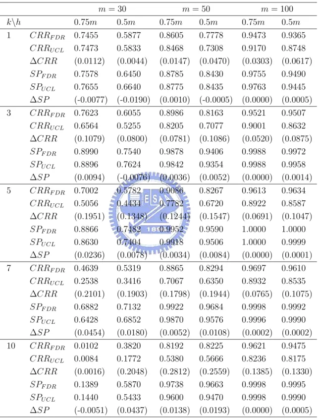
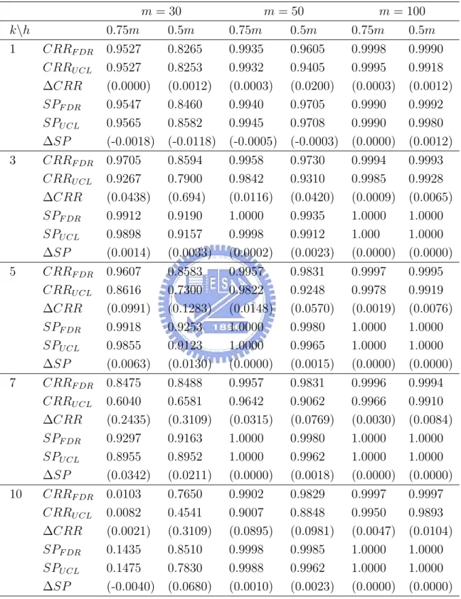
Table 5 gives the results for all combinations of m, k and ncp. “F RRF DR”, “CRRF DR”,

and “SPF DR” denotes respectively the estimates of FRR, CRR, and the signal probability

of the FDR method. If the values are obtained with the T2

mcd control chart, replace the

subscript “FDR” by “UCL”. “∆” denotes the difference of the values between the FDR method and the T2

mcd control chart.

From Table 5, when there are outliers, we see that the detecting power (CRR) of the FDR procedure is better than that of the T2

mcdcontrol chart, while the false-alarm proportion

(FRR) of the FDR procedure is slightly larger than that of the T2

mcd control chart. When

there are no outliers, the false-alarm proportion of the FDR procedure is smaller than that of the T2

mcd control chart.

The simulation results with β_i generated directly from the multivariate normal dis-tribution are given in Table 6 for m=30, 50, 100 under p = 3 and ncp = 49. We find the FDR method is better than the T2

mcd control chart in terms of the CRR value and the signal

probability, and the advantage increases as the number outliers increases, especially for the CRR value. The CRR values for k = 1, 3, 5, 7, 10 are shown in Figures 2-4, in which the differences are evident. In the figures, the symbols “ + ” and “* ” denote 0.75m and 0.5m, respectively, and the solid line is for the FDR method and the dotted line is for the T2

control chart.

From the simulation results, we also find that when choosing h = 0.75m to calculate the T2

mcd statistics, the control schemes not only are more powerful (CRR) but also have

fewer false alarms (FRR) than when choosing h = 0.5m. But when the number of outliers is larger than 0.75m, choosing 0.75m is worse than choosing 0.5m because the MCD estimators are contaminated by outliers. For example, from Figure 2, the CRR value of 0.75m is worse than that of 0.5m when the number of outliers k is larger than 7.

6

Profile Monitoring – Aspartame Example

6.1

A Simulation Study

In this section, to study the effectiveness of two methods with profiles, we analyze the hypothetical aspartame example with model (3.12) given in Subsection 3.3. Figure 1 shows four aspartame profiles generated from model (3.12). The in-control mean vector and the covariance matrix of β_i in the model (3.12) is

β_i ∼ N3(     1 15 1.5    ,     σ2 I 0 0 0 σ2 M 0 0 0 σ2 N    =     0.3 0 0 0 0.5 0 0 0 0.3    ).

Based on model (3.12), we generate the m − k in-control profiles with β_i from the in-control multivariate normal distribution. The k out-control profiles are generated from the out-of-control multivariate normal distribution, where the mean vector µ is shifted to consider the µ_I, µ_M or µ_N. Consider µ_I = (1 + 5σI, 15, 1.5)0 with ncp = 25 or (1 +

7σI, 15, 1.5)0 with ncp = 49, µM = (1, 15 + 5σM, 1.5)0 with ncp = 25 or (1, 15 + 7σM, 1.5)0

with ncp = 49, and µ_N = (1, 15, 1.5 + 5σN)0 with ncp = 25 or (1, 15, 1.5 + 7σN)0 with

ncp = 49.

Our strategy is first to estimate for each profile data the parameter vector in the nonlinear regression model (3.12) with MATLAB. Second, we use the FDR method and the

T2

mcd control chart to monitor the estimates as discussed in the last section. We choose an

overall false-alarm probability α = 0.05, for which the control limits have been provided in Section 5.1.

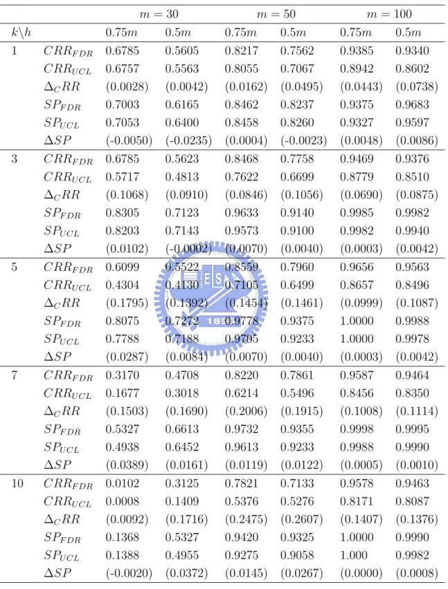
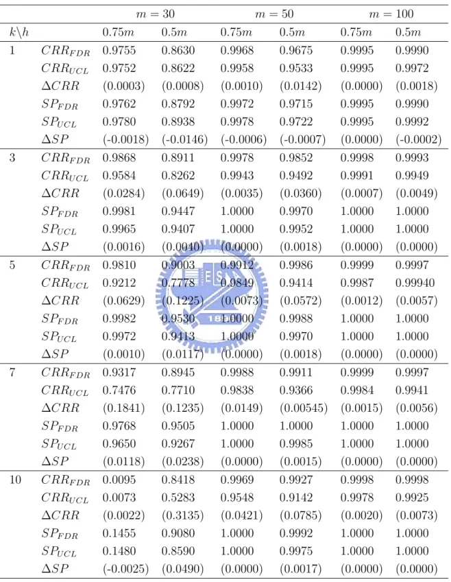
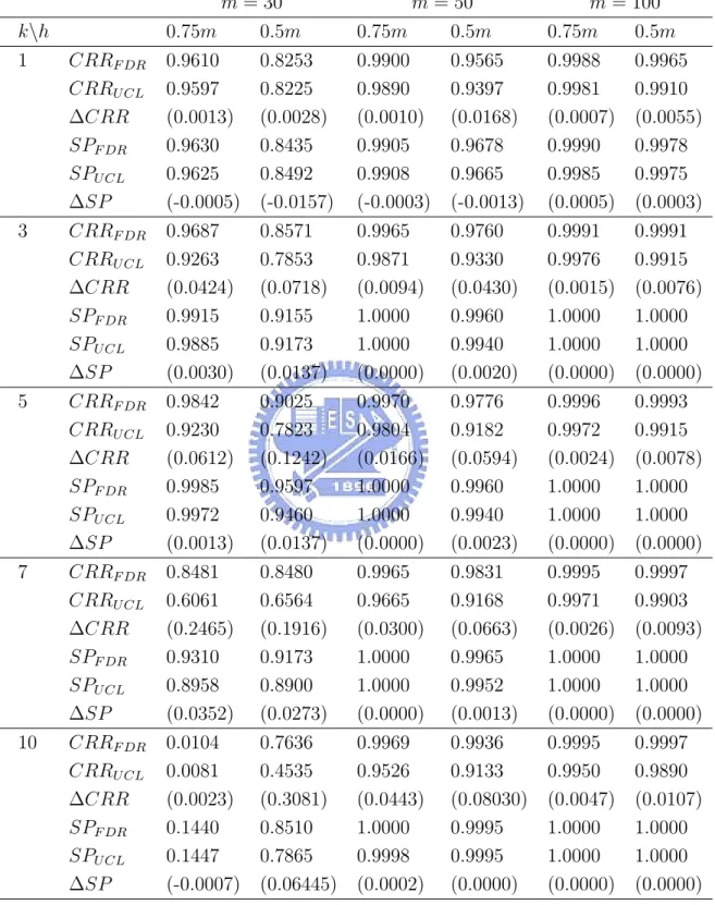
From Table 5, we observe that the FRR values are very small for both monitoring schemes, which indicates that both methods seldom reject in-control samples. To save space, the FRR values of the simulation results are omitted. Table 6 compares the FDR method with T2

i = 1, 2, . . . , m are generated directly from the multivariate normal distribution. We present

in Tables 7-12 the CRR values and the signal probabilities of the FDR method and the T2 mcd

control chart for all combinations of k = 1, 3, 5, 7, 10 and m = 30, 50, 100 with three shifted mean vectors, µ_I, µ_M, and µ_N (two shift sizes each), respectively.

6.2

Results

Comparing the results in Tables 10-12 (ncp = 49) with that in Table 6, we observe that the CRR values with β_iestimated from profiles are both larger than the values with β_i generated directly from the multivariate normal distribution. This indicates that the methods become more sensitive in rejecting samples, i.e., higher detecting power but higher false-alarm rate as well. This may be caused by the estimation error incurred in the non-linear regression.

From Tables 6-12, we see that the power of the FDR method are uniformly better than that of the T2

mcd control chart in terms of the CRR or SP values. Also, we recommend

choosing h = 0.75m to estimate Smcd for the Tmcd2 statistics as long as the percentage of the

outliers is less than 25%. We also observe that the advantage of using the FDR procedure increases as the number of the outliers k outliers increases (with the restriction that k should not exceed the (1 − k/m) level).

Figures 5-22 summarize the CRR results for the various combinations of h, m, k, and the shifted mean vectors µ_I, µ_M and µ_N, with which we can compare the performance of the FDR method and the T2

mcd control chart easily. They also show that the difference between

7

Conclusions

Profile monitoring is a rich and promising area of research. In this paper, we propose a monitoring scheme for nonlinear profiles based on a robust T2 _{statistic and the FDR}

procedure. We consider a nonlinear regression model for profiles with random parameter vector β_i. First, we use the nonlinear regression procedure implemented in MATLAB to estimate the parameter vector of the model for each profile. Then, the estimated parameter vectors can be monitored using the T2

mcd control chart, a robust T2 chart. To improve the

detecting power, the FDR procedure can be employed. Simulation studies show that the proposed FDR scheme outperforms the T2

mcd control chart.

The estimator vector ˆβ_i follows approximately a multivariate normal distribution. So, skipping the nonlinear regression estimation step, we first study the performance of the

T2

mcd control chart and the FDR procedure with βi generated directly from a multivariate

normal distribution. We investigate the effects of m, h, k, and ncp on the performance of the methods. The effects of m and ncp is as expected in the intuitive sense. As expected, the advantage of the FDR procedure increases as k increases, except that k can not exceed the number of samples in the outlying group designed in the MCD procedure. As to h, choosing 0.75m is better than choosing 0.5m with the FDR method and the T2

mcd control chart, when

the dataset contains less than 25% outliers, h = 0.75m may be a good compromise between the breakdown value and the statistical efficiency.

As to profile monitoring, we apply the monitoring schemes to a hypothetical example mimicing the aspartame example given Kang and Albin (2000). We shift the nonlinear parameter mean vectors to µ_I, µ_M, and µ_N with various shift sizes. The conclusions about the proposed methods are similar to that for monitoring multivariate quality characteristic as described above. We also compare the ˆβ_i estimated from profiles to the parameter vector

β_i generated directly from the multivariate normal distribution with the same monitoring schemes proposed in this paper. The monitoring schemes tend to reject more samples when

β_i is estimated by nonlinear regression.

This study extends the framework of statistical process control to more applications. The idea of controlling the False Discovery Rate can be used in the Phase I control chart or any applications involving multiple tests. We believe it can be useful in many applications.

References

[1] Atkinson, A. C. and Mulira, H. M. (1993). “The Stalactite Plot for the Detection of Multivariate Outliers”. Statistics and Computing, 3, 27-35.

[2] Benjamini, Y. and Hochberg, Y. (1995). “Controlling the False Discovert Rate: a Prac-tical and Powerful Approach to Multiple Testing ”. Journal of the Royal StatisPrac-tical

Society: Series B, 57, 289-300.

[3] Brill, R. V. (2001). “A Case Study for Control Charting a Product Quality Measure That is a Continuous Function Over Time”. Presentation at the 45th _{Annual Fall Technical}

Conference, Toronto, Ontario.

[4] Butler, R. W., Davies, P. L., and Jhun, M. (1993). “Asymptotics for the Minimum Covariance Determinant Estimator”. The Annals of Statistics, 21, 1385-1400.

[5] Croux C. and Haesbreck G. (1999). “Influence Function and Efficiency of the Minimum Covariance Determinant Scatter Matrix Estimator”. Journal of Multivariate Analysis, 21, 161-190.

[6] Davis, P. L. (1992). “The Asymptotic of Rousseeuw’s Minimun Volume Ellipsoid Esti-mator”. The Annals of Statistic, 20, 1828-1843.

[7] Ding, Y., Zeng, L., and Zhou, S. Y. (2006). “Phase I Analysis for Monitoring Nonlinear Profiles in Manufacturing Processes”. To appear in Journal of Quality Technology. [8] Gallant, A. R (1987). Nonlinear Statistical Models. New York: Wiley.

[9] Hardin, J. and Rocke, D. (2005).“The Distribution of Robust Distances”. Journal of

[10] Hawkins, D. M. (1994). “A Feasible Solution Algorithm for the Minimum Covariance Determinant Estimator in Multivariate Data”. Computational Statistic and Data

Anal-ysis, 8, 95-107.

[11] Hawkins, D. M. and Merriam, D. F. (1974). “Zonation of Multivariate Sequences of Digitized Geologic Data”. Mathematical Geology, 6, 263-269.

[12] Holmes, D. S. and Mergen, A. E. (1993). “Improving the Performance of the T2 _Control

Chart.” Quality Engineering, 5, 619-625

[13] Jesen, W. A., Birch, J. B., and Woodall. W. H. (2005). “High Breakdown Estimation Methods for Phase I Multivariate Control Charts”. Submitted to Journal of Quality

Technology.

[14] Jensen, W. A., Birch, J. B., and Woodall W. H. (2006). “Profile Monitoring via Linear Mixed Models”. Submitted to Journal of Quality Technology.

[15] Jensen, W. A. and Birch, J. B. (2006). “Profile Monitoring via Nonlinear Mixed Models”. Technical Report No. 06-4, Department of Statistics, Virginia Polytechnic Institute and State University.

[16] Kang, L. and Albin, S. L. (2000). “On-Line Monitoring When the Process Yields a Linear Profile”. Journal of quality Technology 32, 418-426.

[17] Kim, K., Mahmoud, M. A., and Woodall, W. H. (2003). “On The Monitoring of Linear Profiles”. To appear in Journal of Quality Technology.

[18] Lawless, J. F., MacKay, R. J., and Robinson, J. A. (1999). “Analysis of Variation Transmission in Manufacturing Processes—Part I”. Journal of Quality Technology, 31, 131-142.