可應用於多天線系統快速時間同步之研究

國 立 交 通 大 學

資訊科學與工程研究所

碩 士 論 文

可應用於多天線系統快速時間同步之研究

The Study of Fast Timing Recovery For

MIMO-OFDM Systems

研 究 生：呂紹弘

指導教授：陳穎平 教授

可應用於多天線系統快速時間同步之研究

The Study of Fast Timing Recovery For MIMO-OFDM Systems

研 究 生：呂紹弘 Student：Shao-Hung Lu

指導教授：陳穎平 Advisor：Ying-Ping Chen

國 立 交 通 大 學

資 訊 科 學 與 工 程 研 究 所

碩 士 論 文

Submitted to Institute of Computer Science and Engineering College of Computer Science

National Chiao Tung University in partial Fulfillment of the Requirements

for the Degree of Master

in

Computer Science

July 2008

Hsinchu, Taiwan, Republic of China

摘要

近幾年在無線技術發展下，新一代無線通訊系統中，正交分頻多工 (Ortho- gonal Frequency Division Multiplexing, OFDM)已經逐漸變成主流核心，在一個多路徑衰減的 通道中，正交分頻多工被證明能有效的對抗由多路徑衰減所帶來的不理想因素。

本論文主要提出一個可以應用在 IEEE 所制定的無線區域網路標準 IEEE 802.11n 上之時間同步(Timing Synchronization)。其中 IEEE 802.11n 所使用的方式即為多輸入多 輸出正交分頻多工(Multi-Input-Multi-Output Orthogonal Frequency Division Multiplexing), MIMO-OFDM)。

本論文所提出的同步架構著重在時間同步(Timing synchronization)中。主要在試圖 解決在多路徑衰減的通道中，因為通道效應的影響，在接收端所接收到的信號能量會放 大或衰減，而使時間同步產生的取樣判斷上的錯誤.。以一個時脈產生 22 個不同相位的 時序而言，提出的方法將會使最後取樣的相位與理想的相位差距三個相位內。

Abstract

UE to the explosive growth demand for wireless communications, the next-generation wireless communication systems are expected to provide ubiquitous, high-quality, high-speed, reliable, and spectrally-efficient. However, to achieve this objective, several technical challenges have to be overcome attempt to provide high-quality service in this dynamic environment [1].

Orthogonal frequency division multiplexing (OFDM), one of the multi-carrier modulation schemes, turns out to be a strong candidate for the future wideband wireless systems because of its high spectral efficiency and simplicity in equalization. However, OFDM also has its drawbacks. The notable issues of OFDM system are more sensitive to synchronization errors than single carrier system [2], [3]. Most OFDM synchronization methods have one or some of the following limitations or drawbacks: have a limited range of operation, address only one task, have a large estimation variance, lack robust sync detection capability, and require extra overheads [4].

In this work, we introduce a timing synchronization algorithm for 4*4 MIMO-OFDM systems, and try to solve the problem which the signal power will enlarge or decade cause by multi-path channel. This problem will cause sampling phase error. Assume a multiphase generator is used to generate 22 different phases between one clock cycles, the difference between ideal sampling phase and sampling phase determined by this work is 3. Ten L-STS (Legacy Short Training Sequences) are defined in the 802.11n specification, we will perform timing synchronization by used four L-STS in multi-path channel environment and seven L-STS in time variance channel environment. Half L-STS will be used in multi-path channel, and full L-STS will be used in time variance channel.

Acknowledgement

I would like to thank my advisors, Dr. Terng-Yin Hsu and Dr. Ying-Ping Chen, for advice, guidance and constant care. To my dear isIP Lab. members, this work would not have been possible without your support. You make me feel free and comfortable. Always be grateful to my family, your unconditional love encourages me all the time.

Sincerely, Shao-Hung Lu June 2008

Table of Contents

摘要...i

Abstract ...ii

Acknowledgement ... iii

Table of Contents ...iv

List of Figures ...v

Chapter 1 Introduction ...1

Chapter 2 System Platform ...2

2.1 The Basic of OFDM...2

2.2 IEEE 802.11n Physical Layer Specification ...2

2.2.1 Transmitter ...2

2.2.2 Receiver ...3

2.2.3 Basic MIMO PPDU Format...4

2.3 Channel Model...4

2.3.1 Additive White Gaussian Noise ...5

2.3.2 Multipath...5

2.3.3 Time Variant Jakes’ Model...7

2.3.4 Carrier Frequency Offset ...8

2.3.5 System Clock Offset ...9

Chapter 3 Proposed algorithm ... 11

3.1 Timing synchronization introduction... 11

3.2 Timing synchronization algorithm...12

3.2.1 Introduction...12

3.2.2 Proposed algorithm ...14

Chapter 4 Simulation Result ...24

4.1 Simulation Platform ...24

4.2 Simulation Result...25

Chapter 5 Conclusion and Future work ...29

5.1 Conclusion ...29

5.2 Future work...29

List of Figures

Figure 2-1: IEEE 802.11n transmitter data path [7]...3

Figure 2-2: IEEE 802.11n receiver data path...3

Figure 2-3: PPDU Format for NTX antennas [7] ...4

Figure 2-4: OFDM training structure include of L-STF and L-LTF [7] ...4

Figure 2-5: Block diagram of channel model ...5

Figure 2-6: NLOS and LOS between transmitter and receiver...6

Figure 2-7: Instantaneous impulse responses ...7

Figure 2-8: FIR filter with Rayleigh-distributed tap gains at 120km/hr ...8

Figure 2-9: CFO effect under CFO 100 ppm use 64 QAM modulation ...9

Figure 2-10: The sinc waveform of clock drift model effect ...10

Figure 3-1 The block diagram of dynamic sampling... 11

Figure 3-2 The Synchronization Flow ...12

Figure 3-3 Input signal effect by multi-path with no AWGN ...13

Figure 3-4 Input signal effect by multi-path with AWGN in SNR 18dB ...14

Figure 3-5 Illustration boundary idea ...15

Figure 3-6 Cross-correlation architecture ...15

Figure 3-7 Correlation power between P and Phase error ...16 _i Figure 3-8 Down sample at different phase diagram...17

Figure 3-9 Correlation ratios in different phase...17

Figure 3-10 Flow chart of proposed algorithm ...19

Figure 3-11 Proposed algorithm architecture...20

Figure 3-12 The phenomenon of the proposed algorithm in multi-path channel ...20

Figure 3-13 The phenomenon of the proposed algorithm in Time variance channel ...21

Figure 3-14 Exception in this algorithm ...22

Figure 3-15 Sample difference in Multi-path channel 15 taps RMS 100ns...23

Figure 3-16 Sample difference in Time variance channel velocity 120 km/hr 15 taps RMS 100ns ...23

Figure 4-1 : The system performance of 4*4 MIMO-OFDM with 64 QAM, TGn channel E 26 Figure 4-2 : The system performance of 4*4 MIMO-OFDM in Time Variance channel 30km/hr with 64 QAM, TGn channel E ...27 Figure 4-3 : The system performance of 4*4 MIMO-OFDM in Time Variance channel

Chapter 1

Introduction

UE to the explosive growth demand for wireless communications, the next-generation wireless communication systems are expected to provide ubiquitous, high-quality, high-speed, reliable, and spectrally-efficient. However, to achieve this objective, several technical challenges have to be overcome attempt to provide high-quality service in this dynamic environment[1].

Orthogonal frequency division multiplexing (OFDM), one of the multi-carrier modulation schemes, turns out to be a strong candidate for the future wideband wireless systems because of its high spectral efficiency and simplicity in equalization. However, OFDM also has its drawbacks. The notable issues of OFDM system are more sensitive to synchronization errors than single carrier system [2], [3]. Most OFDM synchronization methods have one or some of the following limitations or drawbacks: have a limited range of operation, address only one task, have a large estimation variance, lack robust sync detection capability, and require extra overheads[4].

In this work, we introduce a timing synchronization algorithm for 4*4 MIMO-OFDM systems, and try to solve the problem which the signal power will enlarge or decade cause by multi-path channel. This problem will cause sampling phase error. Assume a multiphase generator is used to generate 22 different phases between one clock cycles, the difference between ideal sampling phase and sampling phase determined by this work is 3.

This thesis is organized as follows. In Chapter 2, a brief introduction of MIMO-OFDM system is given, including IEEE 802.11n physical layer transmitter, receiver and wireless channel model. In Chapter 3, the proposed synchronization algorithm for 4*4 MIMO-OFDM systems is presented. The simulation results are shown in Chapter 4. Finally, this thesis is concluded in Chapter 5 and reference is in the last part of this thesis.

Chapter 2

System Platform

N this chapter, the basic of OFDM is introduced. Three main blocks of wireless communication: transmitter, receiver, and channel model are described as follows.

2.1 The Basic of OFDM

OFDM is a multi-carrier modulation that achieves high data rate and combat multipath fading in wireless networks. The main concept of OFDM is to divide available channel into several orthogonal sub-channels. All of the sub-channels are transmitted simultaneously, thus achieve a high spectral efficiency. Furthermore, sub-carriers have orthogonal property and carried individual data. Their spectrum overlaps are zero. It is easy to use FFT and IFFT to implementation OFDM. However, OFDM has its drawbacks. The significant one is sensitivity to synchronization errors. The synchronization errors come from two sources. One is the local oscillator frequency difference between transmitter and receiver, and the other is the Doppler spread due to the relative motion between the transmitter and the receiver[5]. In addition, timing synchronization may affect the performance of channel estimation[6].

2.2 IEEE 802.11n Physical Layer Specification

2.2.1 Transmitter

The IEEE 802.11n is know as multi-input-multi-output OFDM system (MIMO-OFDM), operating in both 2*2 and 4*4 antennas to transmit and receive data and support higher coding rate up to 5/6. Figure 2-1 shows transmitter data path. First use FEC encoder to encodes the source data. FEC encoder supports 1/2、2/3、3/4、5/6 four kind coding rates. Then

the bit stream is parsed into spatial streams, according to the number of transmit antennas. The interleaver provides a form of diversity to guard against localized corruption or bursts of errors. And then, the QAM mapping is used to modulate the bit stream. It supports BPSK, QPSK, 16 QAM, 64 QAM, 64 QAM or 256 QAM. After QAM mapping, the constellation points pass through Alamouti Space Time Block Code (STBC) encoder. The STBC encoder spreads the constellation points of each spatial stream to any other spatial streams. IFFT is used to transfer signal from frequency domain to time domain. In 20MHz, there are 64 frequency entries for each IFFT, or 64 sub-carriers in each OFDM symbol, 52 of them are data carriers, 4 of them are pilot carriers, other are null carriers. After Insert Guard Interval (GI), the signal is transmitted by RF.

Figure 2-1: IEEE 802.11n transmitter data path [7]

2.2.2 Receiver

Figure 2-2 shows receiver data path. The signal is received form the RF. Sync is used for synchronization, including to find when exactly the packet start, the OFDM symbol boundary and the best sample phase. After a packet is presented, FFT is used to transfer received signal from time domain to frequency domain. Channel effect will be estimated and compensated by Equalizer. IQ mismatch is also taken under consideration. After all estimation and compensation, Alamouti STBC decoder is used to combine four bit streams into original. Then the bit streams are de-map, de-interleaver and merge to single data stream. Finally, it is decoded by FEC which includes de-puncturing, Viterbi decoder and de-scrambler.

spatial merge d e -p un c tur e V iter b id ecode de-scramb le

Figure 2-2: IEEE 802.11n receiver data path

FE C e n c o d e r pu nc tu re frequency interleaver QAM mapping frequency interleaver QAM mapping IFFT IFFT insert GI insert GI analog & RF analog & RF sp a ti a l s tr e a m p a rs e

spatial streams antenna streams

STBC

2.2.3 Basic MIMO PPDU Format

A PHY protocol data unit (PPDU) is defined to provide interoperability. Figure 2-3 shows the PPDU format for the basic MIMO mode. Each packet contains a header (ex. L-STF, L-LTF, …) for detection, channel estimation and synchronization purposes. First part is the L-STF which can be used for signal detection, AGC stabilization, diversity, coarse acquisition …etc. The L-STF is formed by the repetition of ten L-STS of 16 samples each; these samples have correlation properties. In this thesis, correlation techniques will be applicable for packet detection, symbol boundary detection, and timing synchronization. A detail data structure of L-STF is shown as Figure 2-4.

Figure 2-3: PPDU Format for NTX antennas [7]

T1 T2 T3 T4 T5 T6 T7 T8 T9 T10 GI L1 L2 L-STF 8 µs L-LTF 8 µs 16 µs

Figure 2-4: OFDM training structure include of L-STF and L-LTF [7]

2.3 Channel Model

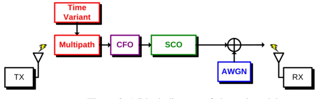
There are many imperfect effects during transmitted signals through channel, such as Additive White Gaussian Noise (AWGN), carrier frequency offset (CFO), multipath, and so on. The block diagram of channel model is shown in Figure 2-5.

Multipath CFO SCO AWGN Time Variant RX TX

Figure 2-5: Block diagram of channel model

2.3.1 Additive White Gaussian Noise

Wideband Gaussian noise comes from many natural sources, such as the thermal vibrations of atoms in antennas, "black body" radiation from the earth and other warm objects, and from celestial sources such as the sun. The AWGN channel is a good model for many satellite and deep space communication links. On the other hand, it is not a good model for most terrestrial links because of multipath, terrain blocking, interference, etc. The signal distorted by AWGN can be derived as

( ) ( ) ( )

r t =s t +n t (2.1)

where r t is received signal, ( ) ( )

s t is transmitted signal, ( )

n t is AWGN.

2.3.2 Multipath

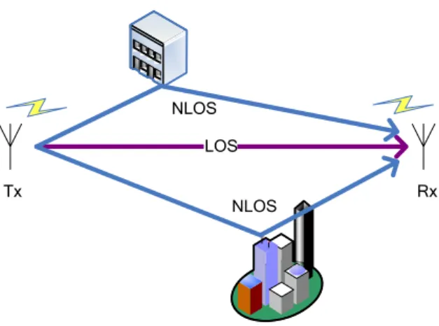
Because there are obstacles and reflectors in the wireless propagation channel, the transmitted signal arrivals at the receiver from various directions over a multiplicity of paths. Such a phenomenon is called multipath. It is an unpredictable set of reflections and/or direct waves each with its own degree of attenuation and delay. Multipath is usually described by two sorts:

A. Line-of-sight (LOS): the direct connection between transmitter and receiver. B. Non-line-of-sight (NLOS): the path arriving after reflection from reflectors.

LOS NLOS

NLOS

Tx Rx

Figure 2-6: NLOS and LOS between transmitter and receiver

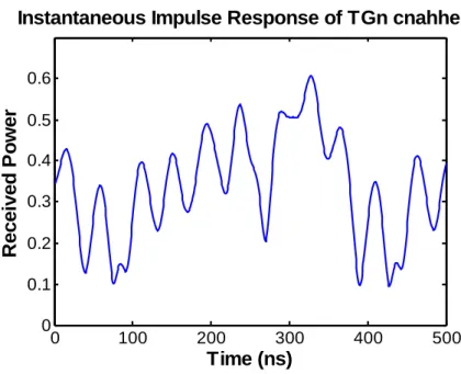
Multipath will cause amplitude and phase fluctuations, and time delay in the received signals. When the waves of multipath signals are out of phase, reduction of the signal strength at the receiver can occur. One such type of reduction is called the multipath fading; the phenomenon is known as “Rayleigh fading” or “fast fading.” Besides, multiple reflections of the transmitted signal may arrive at the receiver at different times; this can result in inter symbol interference (ISI) that the receiver cannot sort out. This time dispersion of the channel is called multipath delay spread which is an important parameter to access the performance capabilities of wireless systems. A common measure of multipath delay spread is the root mean square (RMS) delay spread as shown in Table 2-1. For a reliable communication without using adaptive equalization or other anti-multipath techniques, the transmitted data rate should be much smaller than the inverse of the RMS delay spread (called coherence bandwidth). A representation of Rayleigh fading and a measured received power-delay profile are shown in Figure 2-7.

Table 2-1: TGn multipath channel types [11]

Model LOS/NLOS RMS delay

spread (ns) # of taps A NLOS 0 1 B LOS 15 2 C LOS/NLOS 30 5 D NLOS 50 8 E NLOS 100 15 F NLOS 150 22

0 100 200 300 400 500 0 0.1 0.2 0.3 0.4 0.5 0.6 Time (ns) R e cei v ed P o wer

Instantaneous Impulse Response of TGn cnahhel E

Figure 2-7: Instantaneous impulse responses

2.3.3 Time Variant Jakes’ Model

Time-variant channel effect can be modeled as a FIR filter with time-variant tap gains. For Jakes’ model, the variance of each tap gain obeys Rayleigh distribution. Figure 2-8 shows an n-tap FIR filter with Rayleigh-distributed tap gains, and the corresponded velocity is 120km/hr, shown for 50ms.

Where s t

( )

( )

( )

( ) ( )

∑

The Rayleigh-distributed tap gains w t_k

( )

( )

( )

( )

2 cos cos 2 2 cos cos 2

2 sin cos 2 2 sin cos 2

o o k c c s c N c n n m n N s n n m n w t X t f t X t f t X t f t f t X t f t f t π π β π α π β π α π = = = + = + = +

∑

∑

Figure 2-8: FIR filter with Rayleigh-distributed tap gains at 120km/hr

Where f_c is the carrier frequency, and it equals to 2.4GHz in 802.11n. f_m is the maximum Doppler frequency shift described as

cos

D

f ν θ

λ

≈ ⋅ (2.4)

for θ=0. No is the number of oscillators that generate the sinusoid waveforms of angular

frequency β_n. Detail description of the sum of sinusoids is referred to.

2.3.4 Carrier Frequency Offset

Carrier Frequency Offset (CFO) is caused by the local oscillators’ inconsistency between the transmitter and receiver. The received signals y t can be written as ( )

2

( ) ( ) i ft

t

y t =

∑

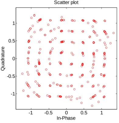
Where Δ and θ are the differences of carrier frequency and carrier phase between TX f and RX, respectively. CFO will cause the constellation of the transmitted signal become a circle, that means phase of the transmitted signal will rotate with time.

( )

( )

Figure 2-9: CFO effect under CFO 100 ppm use 64 QAM modulation

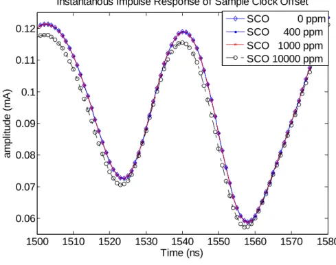
2.3.5 System Clock Offset

The clock drift means the different between the sampling frequency of the digital to analog converter (DAC) and the analog to digital converter (ADC). Because of sampling frequency offset, even if the initial sampling point is optimized, the following sampling points will still slowly shift with time. This model is using compress sinc waveform to cause the clock drift effect, and its effect can be written as

( ) ( ) *sin ( s n) s preADC s s nT T R nT R nT c T − Δ = (2.6)

where R_preADC represents the ADC original output signal,Δ represents shift sampling T_s period and to get R nT signal by convoluting the ADC original output signal and shifted ( s) sinc waveform. Figure 2-10 shows the clock drift model effect. Initial can samples at optimum sampling points, then slightly incorrect sampling instants will cause the SNR degradation. -1 -0.5 0 0.5 1 -1 -0.5 0 0.5 1 Qua d ratur e In-Phase Scatter plot

Figure 2-10: The sinc waveform of clock drift model effect 1500 1510 1520 1530 1540 1550 1560 1570 1580 0.06 0.07 0.08 0.09 0.1 0.11 0.12 Time (ns) am pl it ud e (m A )

Instantanous Impulse Response of Sample Clock Offset SCO 0 ppm SCO 400 ppm SCO 1000 ppm SCO 10000 ppm

Chapter 3

Proposed algorithm

3.1 Timing synchronization introduction

The interface between RF and Baseband data are Digital to Analog Converter (DAC) in the transmitter and Analog to Digital Converter (ADC) in the receiver side. The ADC is the first stage of baseband, so it dominates the receiving signal to noise ratio (SNR). To get the highest input SNR, the ADC is hoped to sample at the eye open position where it has the maximum signal power. However, the initial sampling phase could be anywhere in the eye diagram, so timing synchronization is necessary. The ADC has two kinds of clock source: free running clock and phase lock loop (PLL) output clock. With free running clock, this method also called non-synchronous sampling or fix sampling and there clock frequency and phase are fixed. Once timing error was estimated, the compensation would be performed with the interpolator. With PLL output clock, is also called synchronous sampling or dynamic sampling, the receiver detect the timing error and adjusts its frequency and phase to compensate the error. It is a needed to maintain synchronization while the accuracy and stability of the original clock reference in the receiver is not ideal. Figure 3-1 illustrates the block diagram of dynamic sampling. The clock source is the ADDLL output. ADDLL (All-digital delay lock loop) would adjust the sampling clock frequency and phase directly once the timing error is estimated [12], [13], [14], [15].

ADC

clock

Demodulation

Error estimate ADDLL

Figure 3-1 The block diagram of dynamic sampling

In this thesis, dynamic sampling method is chosen to compensation the error phase. Before timing synchronization, the ADC in the receiver samples the input signal with the

initial phase and then makes the sample clock phase sample correct on the eye open position.

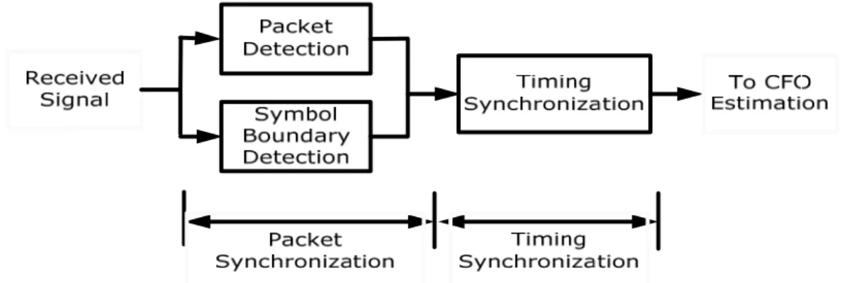
The synchronization flow is shown in Figure 3-2. The packet synchronization simultaneously

perform the correlation and detection distribution in [16], and our algorithm will focus on timing synchronization in this thesis

Figure 3-2 The Synchronization Flow

3.2 Timing synchronization algorithm

3.2.1 Introduction

There are many timing acquisition methods, such as the idea of early-late gate or ML algorithm. All of these methods calculate the correlation power and compare with each other. Those algorithms find out the largest one and adjust the sampling point to where the largest one is. The correlation is to use one preamble signal with fixed form, then use this preamble signal to perform multiply-add operations. The preamble is constructed based on the L-STF (Legacy Short Training Field) in the 802.11n MIMO system. The cross-correlation formula is 1 0 | ( 1) * ( 1) | B i i L P R k B Q k B = =

∑

Where P_i is correlation power, R k_i( ) is received signal, B is short preamble length and

1( ) [ (1) (2) (3) ( 2) ( 1) ( )]

Q k = L−STS L−STS L−STS " L−STS B− L−STS B− L−STS B

(3.2)

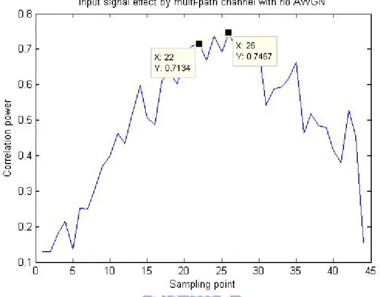
Those methods may suffer some problems in the multi-path channel environment that the sampling point has the largest correlation power may not be the ideal sampling point. In such channel environment, the input signal power maybe degrades or enhances by noise or the summing up the multi-path powers of input signal time delay [8]. Figure 3-3 shows the correlation power affected by multi-path channel in RMS 100ns and 15 taps but without AWGN. In this figure, the correct sampling point is at 22, but the method by select the

maximum correlation power will select at 26 to be the best sampling point. Figure 3-4 shows the correlation power effect by multi-path channel in RMS 100ns, 15 taps and AWGN with SNR 18dB. In this figure, the correct sampling point is at 22, but the method by select the maximum correlation power will select at 29 to be the best sampling point.

Figure 3-4 Input signal effect by multi-path with AWGN in SNR 18dB

3.2.2 Proposed algorithm

The one of idea which we will be used was proposed in [16]. In that, we can adjust the sampling point by use the front boundary and rear boundary of the boundary which is corresponded to with the input signal. The conception of this idea can be explained with a simple example shown in Figure 3-5.

Figure 3-5 Illustration boundary idea

As a real plane like Figure 3-5, the sample point is shifted with time from the left to the right. And the value is sampled from 0.9 to 2.2 through the value 1 and 2. In those value, the sample point at closed to 1 and 2, such as sample point A and B, can get a closed to 1, such as 0.9 or 1.1. We will determine the sample value at sample point A and B to 1 directly, because they are closed to 1. The same thing is happened when sample point is close to 2. But in the sample point like C and D in the middle of 1 and 2. It’s difficult to judge the sample value. If the position of 1 and 2 are the ideal sample points we want to sample. Then it is nearly correct position to sample at the point A, B, E and F. Hence it has the sample value closed to 1 and 2.

Performing this ideal to determine sample point in the system, there are some things to prepare. First, a set of preamble is needed to perform correlation. The preamble is formed by the repetition of ten L-STS of 16 samples each, as the figure 2-4. Consider the boundary correlation buffer (BCB) fill with ideal short training sequence with a cyclic shift like the equation(3.3). 1 2 3 ( ) (1) (2) (3) (14) (15) (16) ( ) ( ) (16) (1) (2) (13) (14) (15) ( ) (15) (16) (1) (12) (13) (14) Q k L STS L STS L STS L STS L STS L STS Q k Q k L STS L STS L STS L STS L STS L STS Q k L STS L STS L STS L STS L STS L STS − − − − − − = = − − − − − − − − − − − − ⎡ ⎤ ⎡ ⎤ ⎢ ⎥ ⎢ ⎥ ⎢ ⎥ ⎢ ⎥ ⎢ _{⎥ ⎣ ⎦} ⎣ ⎦ " " " (3.3)

The input signal will be revised to the form like Q k₂( ) in the equation (3.3) after symbol boundary detection scheme in the system platform. The architecture is like the Figure 3-6. Performing the correlation between the input signal and BCB like the equation (3.1), we can get a set of correlation power. By compare the correlation power with P₁ andP₃, we can adjust to the ideal sample point. The phase error and the correlation power betweenP₁, P₂

and P₃ are shown in Figure 3-7

Correlation

Figure 3-7 Correlation power between P_i and Phase error

Another idea we used was proposed in [15], that tell us how to execute 1x sampling rate acquisition algorithm. Figure 3-8 show the step which sample at different phase in each sampling time. In step1, we sample the input signal at initial phase; step 2 sample the input signal atinitial_ phase+120o, and step 3 sample the input signal at initial_phase+240o. In the step 4, we sample the input signal at initial_ phase+60o, because the correlation power relationship is step1>step2>step3. After 4 steps, the way to adjust sampling point to the ideal sampling point is shown in Figure 3-9. In Figure 3-9, it was according to the ratio of the relationship ofP₁,P₄ and P₂ to adjust the final sampling phase. As the Figure 3-9, A and

B express different ratio betweenP₁,P₄ andP₂. In the Figure 3-9.1, P₂−P₄ ≅P₂ − , this P₁

means sampling point in step4 is correct. In the Figure 3-9.2, P₂−P₄ > P₂− , so need to P₁

adjust the sampling point close to the sampling point in step2. In the Figure 3-9.3, is opposite case shown in Figure 3-9.2.

Figure 3-8 Down sample at different phase diagram

Figure 3-9 Correlation ratios in different phase

In the proposed synchronization algorithm, we will combine the two skills mentioned above but with some modification. In this method, we down sample at different sampling phase and calculate correlation power by equation (3.1), but in proposed timing synchronization algorithm, we use boundary correlation buffer (BCB) Q k( )as equation (3.4). [16] is a good timing synchronization algorithm, but this algorithm depend on the correct result of symbol boundary detection. If the result of symbol boundary detection is wrong, this will affect the timing synchronization. So will use not only three shift preamble, but all of the cyclic shift preamble, like the equation (3.4).

1 2 3 2 1 (1) (2) (3) ( 2) ( 1) ( ) ( ) (16) (1) (2) ( 3) ( 2) ( ) (15) (16) (1) ( ) ( ) ( ) ( ) ( ) " " " " " " " " " # L L L L STS L STS L STS L STS B L STS B L STS B Q k L STS L STS L STS L STS B L STS B L STS Q k L STS L STS L STS Q k Q k Q k Q k Q k − − − − − − − − − − − − − − − − − − − − − = = ⎡ ⎤ ⎢ ⎥ ⎢ ⎥ ⎢ ⎥ ⎢ ⎥ ⎢ ⎥ ⎢ ⎥ ⎢ ⎥ ⎢ ⎥ ⎢ ⎥ ⎣ ⎦ ( 1) ( 4) ( 3) ( 2) # # # % # # # # % # # # % B L STS B L STS B L STS B − − − − − − − (4) (5) (6) (3) (4) # # # # # # # # L STS L STS L STS L STS L STS L ST − − − − − − ( 1) ( 2) ( 3) (5) ( ) ( 1) ( 2) (2) (3) (4) ( 1) ( ) ( 1) " " " " " " " " " L STS B L STS B L STS B S L STS B L STS B L STS B L STS L STS L STS L STS B L STS B L STS B − + − + − + − − + − + − − − − − − − + ⎡ ⎤ ⎢ ⎥ ⎢ ⎥ ⎢ ⎥ ⎢ ⎥ ⎢ ⎥ ⎢ ⎥ ⎢ ⎥ ⎢ ⎥ ⎢ ⎥ ⎢ ⎥ ⎢ ⎥ ⎢ ⎥ ⎣ ⎦ (3.4)

The preamble is continuous and repetition data. With shift and arrange preamble in a BCB array, we can determine the input signal corresponds to what preamble is, for example, if input signal corresponds to Q k₂( ) means the income input signal now most likely

[L−STS(2) L−STS(3) " L−STS B( −1) L−STS B( ) L−STS(1)] and start withL−STS(2). So we will know the input signal starting position correspond to which preamble. Like the step shown in Figure 3-8, and correlation with equation (3.4) by equation (3.1). There is a set of starting position of the preambles in the BCB array. We saved those starting position in an array and called “decision boundary array”. In the “decision boundary array”, we try to find a region called “decision region” which has continuous and the same start position of preamble, because the ideal sampling phase is in this region. The proposed algorithm architecture is shown in Figure 3-11.

The ideal sampling phase is in the “decision region”, and the reason we has explained before. So the “decision boundary array” could be an array like [1 1 ? ? 2 2], and the ideal sample point in the region has continues and the same start position called “decision region”, the array

[

]

[

]

After finding the “decision region”, we have already narrowed down the search range. Then we will try to find ideal sample point in the “decision region”. Up to now, we eliminate those sample point that has the bigger correlation power but not closed to the ideal sampling point. Then we compare those correlation powers in the decision region and choose the one has the maximum correlation power in the decision region. Because the sample point in the “decision region” are possible to be ideal sample point, but the one with the max correlation power is maximum likely.

Figure 3-10 Flow chart of proposed algorithm

Figure 3-12 distribute this phenomenon in multi-path channel, SNR 18dB. The ideal

sample point is located in the _ 1

6

ini phase+ π , but the maximum power is in the

_

ini phase+ . π

In our proposed algorithm, the decision region is _ _ 1

6

ini phase ini phase π

⎡ ₊ ⎤

⎢ ⎥

⎣ ⎦, and

the sampling point we will determine is in the _ 1

6

ini phase+ π . The sample point we

Figure 3-11 Proposed algorithm architecture

Figure 3-13 The phenomenon of the proposed algorithm in Time variance channel

Figure 3-13 distribute this phenomenon in time variance channel. The velocity is 120 km/hr, 15 taps, RMS 100ns, SNR 18dB. The ideal sample point is located in

the _ 5

6

ini phase+ π, but the maximum correlation power is in the ini_phase+ . π

In our proposed algorithm, there will be two decision regions here. One

is _ 1 _ 1 _ 1

6 3 2

ini phase π ini phase π ini phase π

⎡ _{+ + +} ⎤

⎢ ⎥

⎣ ⎦ because their boundary

information is the same, 9 and their correlation power is [0.389 0.3345 0.3395]. The other

is _ 2 _ 5

3 6

ini phase π ini phase π

⎡ ₊ ⎤

⎢ ⎥

⎣ ⎦ because their boundary information is the same, 5

and their correlation power is [0.3771 0.3995]. The maximum power in the two decision region is 0.389 and 0.3995, compared with the two maximum correlation power in each decision region. We will choose that decision region which the maximum power and it is

0.3995. The finial sampling point we will determine is in the _ 5

6

ini phase+ π, this sample

point we determined is the same with ideal sample point.

Some expectant situations may happen in this algorithm. In the proposed algorithm, we need to find “decision region” first. How should we do if there are many “decision region” exist at the same time or there is no any decision region? In the first situation, the way to

choose decision region is finding the maximum correlation power in each decision, and the region has the maximum correlation power between each region is what we want. Then repeat algorithm mentioned above. Figure 3-13 also describe about this.

In the second situation, there are two possible situations but can be recognized as the same situation, cannot find any “decision region” in “boundary decision array”. One is that no continuous and the same start position and another is that have the same start position but not continuous. We solve this problem by comparing the correlation power straightforward, and choosing the one have maximum correlation power. The two situations are shown in Figure 3-14. In Figure 3-14.1 can find two decision regions and we need to specify one. In Figure 3-14.2 we cannot find any decision region in decision boundary array.

Figure 3-14 Exception in this algorithm

Figure 3-15 shows the difference between the sample point which we determined and the ideal sample point. We count total 1500 packets in multi-path channel with 15 taps, RMS 100ns. The RMSE (root mean square error) is 2.653, this shows that in general speaking the difference between the samples points whose we determined and the ideal sample point is 2.653. The equation of RMSE is

2 1 1 ( _ _ ) N i

RMSE Sampling phase Ideal phase

N =

=

∑

And Figure 3-16 shows the difference between the sample point which we determined and the ideal sample point. We count total 1500 packets in time variance channel with 15 taps, RMS 100ns, and velocity 120 km/hr. The RMSE (root mean square error) is 2.653. This show that the difference between the sample point we determined and the ideal sample point is 2.930.

Figure 3-15 Sample difference in Multi-path channel 15 taps RMS 100ns

Figure 3-16 Sample difference in Time variance channel velocity 120 km/hr 15 taps RMS 100ns

Chapter 4

Simulation Result

E use simulation to evaluate the receiver’s performance with the AWGN, Multi-path fading and time variance channel effect. We can express the received signal sample as:

(

)

Where the H k is the multipath with time-variant model, the exponential term is CFO _ij( )

effect, the sinc part is SCO effect and N k is AWGN. _ij( )

4.1 Simulation Platform

MATLAB is chosen as simulation language, due to its ability to mathematics, such as matrix operation, numerous math functions, and easily drawing figures. A MIMO-OFDM system based on IEEE 802.11n Wireless LANs, TGn Sync Proposal Technical Specification, is used as the reference simulation platform. The major parameters are shown in Table 4-1.

Table 4-1 Simulation parameters

Parameter Value

MCS Set 27 / 29

Antenna No. 4*4

Modulation 16 QAM / 64 QAM

Coding Rate 2/3

PSDU Length 1024 Bytes

Carrier Frequency 2.4 GHz

Bandwidth 20 MHz

IFFT / FFT Period 3.2 sμ

4.2 Simulation Result

As mention before, the multiphase generator is used to generate 22 phases between one clock cycles. In other word, the phase error 22 means that signal is delay one cycle, and the phase error 0 means that sign is at ideal phase.

With different initial phase errors, after timing synchronization, including coarse and fine timing synchronization, the final phase errors are convergence into 3 phases. As shown in Figure 3-15 and Figure 3-16.

Next we will show the performance under the simulation platform defined in Table 4.1. First, consider with the 4*4 MIMO-OFDM system with 64 QAM modulation and TGn channel E (RMS=100ns, Tap=15). The performances are shown in Figure 4-1. The legend ideal sample means to get each sample at right phase (phase error 0). This work sample means use the proposed algorithm in section 3.2 with an unknown initial phase errors to get sample. No synchronization sample means without an algorithm to fix the error of an unknown initial phase.

Figure 4-1-(a) shows the required SNR is 19dB, lost about 1 dB when compare with the ideal sampling. Take the SCO effect into consideration, the required SNR with SCO 400 ppm is about 20dB, lost about 2 dB when compare with no SCO effect. Figure 4-1 -(b) shows the proposed algorithm can tolerance SCO effect about 400 ppm.

Then, consider with the 4*4 MIMO-OFDM system in Time Variance channel with 64 QAM modulation and TGn channel E (RMS=100ns, Tap=15). The performances are shown in Figure 4-2 and Figure 4-3. Figure 4-2-(a) shows the required SNR is about 29 dB in Time variance channel with velocity 30km/hr, lost about 1.2 dB when compare with the ideal sampling. Take the SCO effect into consideration, the required SNR with SCO 400 ppm is about 31dB, lost about 3.5 dB when compare with no SCO effect. Figure 4-2-(b) shows the proposed algorithm can tolerance SCO affect about 400 ppm.

Figure 4-3-(a) shows the required SNR is about 31 dB in Time variance channel with velocity 120km/hr, lost about 1.5 dB when compare with the ideal sampling. Take the SCO effect into consideration, the required SNR with SCO 400 ppm is about 32dB, lost about 2 dB when compare with no SCO effect. Figure 4-3-(b) shows the proposed algorithm can tolerance SCO affect about 400 ppm.

(a) PER vs. SNR

(a) PER vs. SNR

(b) PER vs. SCO

Figure 4-2 : The system performance of 4*4 MIMO-OFDM in Time Variance channel 30km/hr with 64 QAM, TGn channel E

(a) PER vs. SNR

(b) PER vs. SCO

Figure 4-3 : The system performance of 4*4 MIMO-OFDM in Time Variance channel 120km/hr with 64 QAM, TGn channel E

Chapter 5

Conclusion and Future work

N this thesis, based on the preamble structure of IEEE 802.11n standard, a synchronization algorithm for IEEE 802.11n WLANs over TGN channels is proposed. A realistic channel model was employed, which includes the effects of Time variance channel, sampling clock offset, etc. Loss in system performance due to synchronization error was used as a performance criterion.

5.1 Conclusion

We compare other methods with the proposed algorithm in section 3-2. Due to the reason of lack time, we compare two other methods in our system platform. The major improve is in the converge SNR. The comparison is listed in Table 5.1

5.2 Future work

In this thesis, we proposed a method to solve the synchronization problem cause by the multi-path channel. In the time variance channel, it has the same problem like the multi-path channel, but there is still some other problem need to solve. Some other situations can cause synchronization error, like the boundary detection error, Doppler Effect and serious fading by SCO. Otherwise, man-made noise is also a source to affect the accuracy of timing synchronization. Those problems need to be solved in the future.

As to the system, high QAM constellation likes 256-QAM for higher data rate is going to be deployed. Then, more antennas of transmitter and receiver like 8*8 are taken into consideration. Even huge FFT/IFFT (size bigger than 1000) is also a good research topic.

[15] [16] This work

Method ML base Boundary base ML + Boundary base

Converge SNR (100ns 15taps) 21 dB 20 dB 19 dB Converge SNR (Time variance 30km/hr 100ns 15taps)

N/A Can’t converge 29 dB

Converge SNR (Time variance 120km/hr 100ns

15taps)

N/A Can’t converge 31 dB

Control Factor Phase

(32 phases) Phase (22 phases) Phase (22 phases) Over Sampling 1x 1x 1x

Converge Cycle 4 symbols 1 symbols 4 symbols

Bibliography

[1] T. Ojanperá and R. Prasad, "An overview of wireless broadband communications", IEEE Commun. Mag., vol. 35, pp. 28-34, Jan. 1997.

[2] T. Pollet, M. Van Bladel, and M. Moeneclaey, “BER sensitivity of OFDM systems to carrier frequency offset and Wiener phase noise”, IEEE Trans. Commun., vol. 43, pp. 191-193, Feb./Mar./Apr. 1995 .

[3] M. Gudmundson and P.O. Anderson, “Adjacent channel interference in an OFDM system”, in Proc. Vehicular Technol. Conf., Atlanta, GA, May 1996, pp. 918-922.

[4] H. Minn, V. K. Bhargava, K. B. Letaief, “A robust timing and frequency synchronization for OFDM systems”, IEEE Trans. on wireless Commun., vol. 2, pp. 822-839, No. 4, July 2003.

[5] Hao Zhou, Malipatil A.V., Yih-Fang Huang, “Synchronization Issues in OFDM

Systems”, Circuits and Systems, APCCAS 2006, pp. 988-991, Dec 2006

[6] M. Speth, S. Fechtel, G. Fock, and H. Meyr, “Optimum Receiver Design for Wireless Broad-Band Systems Using OFDM – Part I”, in IEEE Trans. on Comm., vol. 47, no. 11, pp. 1668-1677, Nov.1999.

[7] 802.11n standard, “TGn Sync Proposal Technical Specification”, IEEE 802.11-04/0889r7, July 2005.

[8] Theodore S.Rappaport, “Wireless Communications PRINCIPLES AND PRACTICE SECOND EDITION”, Prentice Hall PTR 2002, pp185~191.

[9] P. Dent, G. Bottomley and T. Croft, “Jakes Fading Model Revisited”, IEE Electronics Letters, p.1162~p.1163, June 1993

[10] W. C. Jakes, Ed., “Microwave Mobile Communications”, IEEE Press, Piscataway, NJ, 1974

[11] IEEEE P802.11 Wireless LANs, “Indoor MIMO WLAN Channel Models (Draft Document in Progerss_Rev1)”, IEEE 802.11-03/161r1, July 11, 2003.

[12] J.Y. Yu, C.C. Chung, H.Y. Liu, and C.Y. Lee, “Power Reduction with Dynamic Sampling and All-Digital I/Q-Mismatch Calibration for A MB-OFDM UWB Baseband Transceiver,” IEEE Symposium on VLSI Citcuits, June 2006.

[13] S. Sibecas, C.A. Emami, G. Stratis, and G. Rasor, “Pseudo-Pilot OFDM scheme for 802.11a and R/A in DSRC Applications,” IEEE VTS-Fall, VTC, Oct 2003.

Systems,” IEEE Trans. Broadcasting, vol. 50, pp. 56-62, March 2004.

[15] Terng-Yin Hsu, You-Hsien Lin and Ming-Feng Shen, ” Synchronous Sampling Recovery with All-Digital Clock Management in OFDM Systems”, 2007

[16] I-Yin Liu, “The Study of Front-end Signaling and Timing Synchronization in MIMO-OFDM systems”, NCTU, master thesis, June 2007