建立OOMPNets之開發環境

全文

(1)國立交通大學資訊科學與工程研究所碩士論文. 建立. O O M P N e t s. 之開發環境. Constructing a Development Environment for OOMPNets. 研究生：何立中指導教授：王豐堅. 教授. 中華民國九十七年八月.

(2) 建立 OOMPNets 之開發環境 Constructing a Development Environment for OOMPNets. 研究生：何立中. Student：Li-Chung Ho. 指導教授：王豐堅. Advisor：Feng-Jian Wang. 國立交通大學資訊科學與工程研究所碩士論文. A Thesis Submitted to Institute of Computer Science and Engineering College of Computer Science National Chiao Tung University in partial Fulfillment of the Requirements for the Degree of Master in. Computer Science August 2008. Hsinchu, Taiwan, Republic of China. 中華民國九十七年八月.

(3) 建立 OOMPNets 之開發環境. 研究生: 何立中. 指導教授: 王豐堅博士. 國立交通大學資訊科學與工程研究所碩士論文. 摘要. 著色派翠網是一種可以被用來分析許多系統的模型，而物件導向技術在近年廣泛的被使用，我們實驗室結合著色派翠網和物件的概念而發展出來一個物件導向模組化派翠網的模型。物件導向模組化派翠網減少由模型轉換為物件導向概念的時間，也正提出了一個物件導向模組化派翠網的開發環境，裡面包含了一系列的工具。本論文實作物件導向模組化派翠網的編輯器和一個相對應的發生圖的分析工具。編輯器提供了一些檢查避免不正常的現象存在於模型中，以減輕使用者的負擔。而後者，則藉著轉換演算法之轉換，利用將物件導向模組化派翠網轉換成著色派翠網，並使用已存在的分析方法做分析，再將分析的結果對應到轉換前的物件導向模組化派翠網，藉此達到分析物件導向模組化派翠網的目的。. 關鍵字：著色派翠網，物件導向技術，轉換演算法，編輯器，分析，開發環境. i.

(4) Constructing a Development Environment for OOMPNets Student: Li-Chung Ho. Advisor: Dr. Feng-Jian Wang. Institute of Computer Science and Engineering National Chiao Tung University 1001 Ta Hsueh Road, Hsinchu, Taiwan, ROC. Abstract. Colored petri nets (CPNs) is a kind of model which can be used to analyze many kinds of systems. Object oriented (OO) techniques, including analysis, design and programming, are popular for years. Object oriented modular petri nets (OOMPNets), proposed by our laboratory, is a model extended from CPNs by integrating object concept into CPNs. Our laboratory is now developing the development environment which consists of a series of tools to help simplify the development of OOMPNets. This thesis implements part of the environment, including an editor named OOMPNE and a transformation tool. OOMPNE is used for constructing OOMPNets. OOMPNE provides some checks to reduce the abnormal phenomena occurring in the modeling OOMPNet. The analysis is done by transferring the modeled OOMPNets into CPNs and calling the existing analysis methods of based on occurrence graph in CPNs. We also discuss the techniques to locate the defect(s) and corresponding object/place(s) in original OOMPNets, corresponding to the defects found in above analysis.. Keywords: Colored petri nets, object oriented modular petri nets, analysis. ii.

(5) 誌謝. 本篇論文的完成，首先要感謝我的指導教授王豐堅博士不斷的指導與鼓勵，讓我在軟體工程的測試技術上，得到很多豐富的知識與經驗。另外，也非常感謝我的畢業口試評審委員朱正忠博士、留忠賢博士與黃俊龍博士，提供許多寶貴的意見，補足我論文裡不足的部分。. 其次，我要感謝實驗室的學長姐們，有博士班靜慧學姐與懷中學長的指導與照顧，讓我學到許多做研究的技巧，得以順利完成論文。. 最後，我要感謝我的家人，由於你們的支持，讓我能心無旁騖地讀書，專心做研究。由衷地感謝你們大家一路下來陪著我走過這段研究生歲月。. iii.

(6) Table of Contents 摘要…………………………………………………………………………………....i Abstract………………………………………………………………………………..ii 誌謝…………………………………………………………………………………...iii Table of Contents…………………………………………………………………......iv List of Figures and Tables………………………………………………………….....vi Chapter 1. Introduction……………………………………………….……..….……..1 Chapter 2. Background……………………………………………….………...……..3 2.1. Colored Petri Nets…………………………………………….………………..3 2.2. Object Oriented Modular Petri Nets………………….……….……………….8 2.2.1. The Extensions of Places and Transitions..................................................8 2.2.2. The Extensions of Tokens.........................................................................10 2.2.3. Synchronization Relation and Share Node...............................................10 2.2.4. Formal Definition of OOMPNets.............................................................12 Chapter 3. An Editor for OOMPNets.....……………………………………………..14 3.1. Edit Functions in OOMPNE.....………………………...…………………….15 3.2. Basic Abnormal Phenomena..................……………………………………...22 3.3. Incremental Analysis for the Anomalies in OOMPNE....................................25 Chapter 4. Technology of Analyzing OOMPNets..............................................…....30 4.1. The Mechanisms of Transformation Algorithm............………………...……30 4.2. Transformation Algorithm....……………………………………………….....42 Chapter 5. Example....................................................................…………………….52 5.1 Edit OOMPNets with OOMPNE......................................................................52 5.2 Analyzer in OOMPNets, OOMPOA.................................................................60 Chapter 6. Conclusion and Future Works....................................................................67 iv.

(7) Reference…………………………………………………………………………....68. v.

(8) List of Figures and Tables Figure 3-1 The window in OOMPNE...…………………………………………..14 Figure 3-2 The windows in editing token properties and variables.......…………16 Figure 3-3 The popup menu of right click a place.......…………………………..17 Figure 3-4 The popup menu of operation duplicate....................………………..17 Figure 3-5 The popup menu of a transition..............…………………………….19 Figure 3-6 The popup menu of an input arc.....………………………………….20 Figure 3-7 The window in editing tokens………………………………….........21 Figure 3-8 The reaction from OOMPNE of deleting used color set(s)…..…...…25 Figure 3-9 The net after deleting transition T0 in Figure 3-8.................…..……26 Figure 3-10 (a) the destination changed into turning point when user connects two places. (b) the turning point is shown by moving place P1…......…26 Figure 3-11 The window in editing input arc expression.......................………..27 Figure 3-12 (a) and (b) show the reminding ways of OOMPNE when user’s action violates the rules….......................................................................…28 Figure 4-1 The hierarchical tree structure of an OOMPNet net 0………..……....36 Figure 4-2 An OOMPNet SN contains two object-nets.…………………………39 Figure 5-1 The window of declaring color sets...................................…...……..54 Figure 5-2 The OOMPNet of color set ATM.....................……………………...54 Figure 5-3 The window of declaring variables......………………………………55 Figure 5-4 The warning message of editing unbalance inscriptions of arc (Start, Provide information to identify the identity)...........................56 Figure 5-5 The OOMPNet of scenario “transfer account successfully”...............56 Figure 5-6 The OOMPNet of refinement described in Table 5-3.........................58 Figure 5-7 The OOMPNet of refinement described in Table 5-4.........................59 vi.

(9) Figure 5-8 The OOMPNet of scenario “transfer account successfully”...............60 Figure 5-9 T-CPN of OOMPNet in Figure 5-5.....................................................62 Figure 5-10 The occurrence graph of T-CPN in Figure 5-9..................................62 Figure 5-11 The best integer bounds of the T-CPN...............................................63 Figure 5-12 The best multi-set bounds of the T-CPN............................................64 Figure 5-13 The home properties of the T-CPN.....................................................65 Figure 5-14 The liveness properties of the T-CPN.................................................66 Algorithm 4.1 OOMPNetToCPN…………………………………….…...……….43 Algorithm 4.2 CreateTransition............………………………………….………..47 Algorithm 4.3 ProduceElement..............................................................................48 Algorithm 4.4 CreateSTG.......................................................................................49 Table 5-1 The specification of “Transfer Account”.....................…………………52 Table 5-2 The scenario of “Transfer Account Successfully”…...………………….53 Table 5-3 The refinement of transition “Provide information to identify the identity”...................................................................................................57 Table 5-4 The refinement of transition “transfer account”….......…………………58. vii.

(10) Chapter 1. Introduction. Object Oriented Modular Petri Nets (OOMPNets) developed in our laboratory is a model which can be represented with a sequence of graphs or mathematical formulas, where the former is more readable. OOMPNets is extended from Colored Petri Nets (CPNs) with object concept. This is achieved by allowing 1) a net to be a token of another one, 2) nodes to be refined with nets and 3) nets to be combined with shared nodes. OOMPNets contains the three distinct properties: 1) For one object-net, the internal relationships of tokens encapsulated and the ripple-effect reactions caused from external firing transitions are totally represented, 2) Refineable nodes encapsulate the information with internal hierarchical presentation and 3) The nets can be combined flexibly gives a fit expression to serve developers who concern specific problems.. Currently, our laboratory is developing an environment to help the development of OOMPNets. This thesis provides two parts of the development environment: OOMPNE and OOMPOA are provided to edit and analyze OOMPNets, respectively. OOMPNE is extended from a Petri Net editor, PIPE2 [3]. OOMPNE consists of a set of edition activities to reduce the abnormal phenomena appearing in the modeled net during edit. OOMPNE also provides some simple checks to help user find the defect earlier, e.g. arc expression unbalance. In summary, OOMPNE helps user to model an OOMPNets without fundamental errors, e.g. undefined color sets used, shared node with different labels and arc expression unbalance. OOMPNE might reduce the time of modeling well-form OOMPNets, since some abnormal phenomena are prevented.. 1.

(11) There is no analysis method developed for OOMPNets yet. An OOMPOA provided in this thesis is used to analyze OOMPNets with occurrence graph. OOMPOA analyzes OOMPNets with four steps: 1) transform OOMPNets into CPNs, 2) construct the occurrence graph of the CPNs transformed from OOMPNets, 3) investigate the dynamic properties of the occurrence graph to analyze the CPNs and 4) map the analysis results back to OOMPNets. According to the transformation information provided in OOMPOA, the dynamic properties for OOMPNets can be studied further. Besides, the information can help to develop analysis method for OOMPNets.. The rest of this thesis is organized as follows. Chapter 2 introduces CPNs and OOMPNets. The capabilities and checks of OOMPNE are described in Chapter 3. The technology of analyzing OOMPNets is introduced in Chapter 4. Chapter 5 uses an example to show how to use OOMPOA to analyze OOMPNets. Chapter 6 concludes the thesis and indicates some future works.. 2.

(12) Chapter 2. Background. This chapter introduces Colored Petri Nets (CPNs) in Section 2.1. The Object Oriented Modular Petri Nets (OOMPNets) is introduced in Section 2.2.. 2.1. Colored Petri Nets. The definition of CPNs given in Definition 2-1 is modified from the one presented in [1] with a variable tuple V.. Definition 2-1 (Colored Petri Net): A Colored Petri Net is a 9-tuple CPN  (,V , P, T , F , C , G, A, I ) satisfying the requirements below: (1) Σ is a finite set of non-empty types, called color sets. (2) V is a set of variables. Variables are used to describe the guard expressions of transitions and the expressions of arcs. (3) P is a finite set of places. (4) T is a finite set of transitions. (5) F is a finite set of arcs such that:. P T  P  F  T  F   (6) C is a color function. It is defined from P into Σ. (7) G is a guard function. It is defined from T into expressions such that: t  T : [Type( G( t ))  Βoolean  Type(Var( G( t )))   ]. where Type(Var(G(t))) represents the types of variables applied in G(t), Type(G(t)) represents the type of value after G(t) is executed. (8) A is an arc expression function. It is defined from F into expressions such that: f  F : [Type( A( f ))  C( p( f ))  Type(Var( A( f )))   ]. 3.

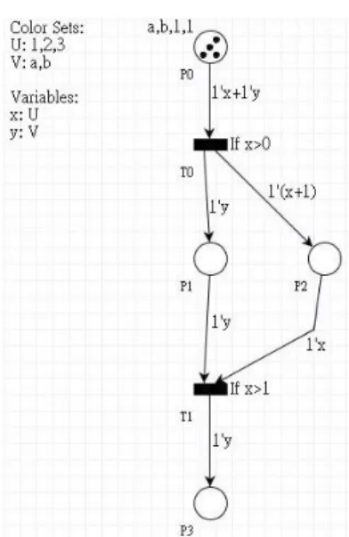
(13) where p(f) is the place node of arc f. (9) I is an initialization function. I is defined from P into closed expressions 1 such that: p  P : [Type( I( p ))  C( p )]. The elements defined in Definition 2-1 are illustrated with a net CPN one by one. Let CPN be (,V , P, T , F , C , G, A, I ) , where (1) If place p, p  P , holds set of tokens D, then.  Type(d )  C ( p) .. d D. (2) The variable type of v, v V , belongs to Σ, denoted as Type(v)   . (3) A marking, a multi-set of net’s places, of CPN denotes a state of the net. (4) Firing a transition t, t T , changes state m to m’. m could equal to m’. (5) f1 , f 2 , f1 and f 2  F , N ( f1 )  N ( f 2 ) 2. (6) Color function C maps p, p  P , to a set of types. (7) The guard expression of transition t, t T , return a boolean value b. When b is true, transition t is enables. (8) The variable types involved in arc expression A( f ) are contained in C ( p( f )) . (9) The initial marking generated by I for p  P is restricted to satisfy the types defined by all corresponding C ( p ) .. A CPN is a directed graph. An example net CPN composed if four places and two transitions is shown in Figure 2-1. The initial marking M0 of CPN is (p0(a,b,1,1),p1,p2,p3). The net is defined with two color sets (types) U and V. The value of U type element (variable or token) is 1, 2, or 3. The value of V type element is a or b. Variable x and y used in the net are declared with U and V type, respectively.. 1 2. An expression without variables is said to be a closed expression. N is a node function. It is defined from A into P× T∪T× P. 4.

(14) Each transition or arc is associated with an expression, which is composed of variables or elements in color set above, respectively.. Figure 2-1 A simple example of CPNs.. The behaviors of CPNs are defined in Definition 2-3, 2-4 and 2-5: Definition 2-2 A token element is a pair ( p,c ) where p  P and c  C( p ) , while a binding element is a pair ( t ,b ) where t T and b  B( t ) 3. The set of all token elements is denoted by TE while the set of all binding elements is denoted by BE. Definition 2-3 A marking is a multi-set over TE while a step is a non-empty and finite multi-set over BE. The initial marking M0 is the marking which is obtained by evaluating the initialization expressions:. ( p,c ) TE : M 0( p,c )  ( I( p ))( c ). The set of all markings and steps are denoted by M and Y, respectively. A step Y is enabled in a marking M iff the following property is satisfied:. 3. B(t) is the set of all bindings for t. 5.

(15) p  P :. . A( p,t )  b   M( p ). ( t ,b )Y. Let the step Y be enabled in the marking M. When ( t,b )  Y , we say that t is enabled in M for the binding b. We also say that ( t ,b ) is enabled in M, and so is t.. If a transition t is firable in a marking M, there are two properties needed to be satisfied: (1) The evaluation result of G(t) based on a binding b is true (2). p  P :. . A( p,t )  b   M( p ) .. ( t ,b )Y. Definition 2-4 When a step Y is enabled in a marking M1, the marking change from M1 to M2 can be defined as:. p  P : M 2 ( p )  ( M1( p ) . . A( p,t )  b  ) . ( t ,b )Y. . A( t, p )  b . ( t ,b )Y. The first sum represents the tokens removed while the second for the token added. Moreover, we say that M2 is directly reachable from M1 by the occurrence of the step Y, which we also denote: M1 [Y  M 2 .. The expressions of an input arc of a place describe that tokens are added into the place when the corresponding transition is occurred. The tokens are removed from a place are described in the expressions of the output arc of the place. When a transition t fires, the tokens of corresponding places are added or removed. The addition and removing tokens is basing on the corresponding arc expressions and binding of the occurring step.. Definition 2-5 A marking is a multi-set over P while a step is a non-empty and finite multi-set over T. The initial marking M0 is the marking which is obtained from the initialization expressions:. p  P : M 0 ( p )  I( p ). 6.

(16) The sets of all markings and steps are denoted by M and Y, respectively.. CPNs can be analyzed in four different ways [10]. The first analysis method is interactive simulation. This means that user can use the simulator associated with the editor make simulation to investigate the behavior of the modeled system. The second analysis method is automatic simulation. It allows a fast simulation of thousands or millions of transitions. The purpose is to investigate the functional correctness of the system or to investigate the performance of the system, e.g. to identify bottlenecks, to predict the use of buffer space or the mean/maximal service time …, etc. The third analysis method is occurrence graphs (also called state spaces or reachability graphs). The basic idea behind occurrence graphs is to construct a directed graph which has a node for each reachable system state and an arc for each possible state change. Occurrence graph presents all possible states of the modeled system with initial parameters. All step changes of the modeled system are also recorded in the occurrence graph. User investigates the dynamic properties through the occurrence graph. The investigated results help user to find the run-time error(s) embedded in the modeled system. Obviously, such a graph may become very large, even for small CPNs. However, it can be constructed and analyzed totally automatically, and there are techniques working with condensed occurrence graphs without losing analytic power. These techniques are built upon equivalence classes. The fourth analysis method is place invariants. User constructs a set of equations which is proved to be satisfied for all reachable system states. The equations are used to prove some properties of the modeled system, e.g., absence of deadlock.. 7.

(17) 2.2. Object Oriented Modular Petri Nets. OOMPNet is an extension of CPNs. There are three extensions and two new relations in OOMPNets. OOMPNets extends 3 elements in CPNs, places, transitions and tokens. Synchronization relation (SR) and share nodes are provided in OOMPNets. Besides above three extensions and two relations, the remaining parts of OOMPNets are the same to CPNs. The extensions of places and transitions are introduced in section 2.2.1. Section 2.2.2 introduces the extension of tokens. Two new relations, SR and share nodes, are introduced in Section 2.2.3. Finally, a formal definition for OOMPNets is described in Section 2.2.4.. 2.2.1. The Extensions of Places and Transitions. The places are separated into two sets, primary and abstract places in OOMPNets. The primary places are defined the same as places in CPNs. The abstract places are clarified further with refinement nets rPNet, as in Function 2-1.. Function 2-1 (refinement of abstract place): An. abstract. place. p. can. be. refined. as. an. OOMPNets. rPNet  (' ,V ' , P' , T ' , D' , F ' , C' , G' , A' , I ' , L' ) , where: 1. P'  { pin , pout }  P'' . The input and output transitions of p are transferred to pin and pout respectively, where. In( p)  In( pin )  {t T | f  F : N ( f )  (t , p)} Out ( p)  Out ( pin )  {t T | f  F : N ( f )  ( p, t )} 8.

(18) 2. If P''  , F '  ( pin  T ' )  (T '  pout ) . 3. If P ''   1). T '  T ''  T1  T2 and the intersection of each pair is  , and. 2). F '  ( pin  T1 )  (T2  pout )  ((T ''  T1 )  P'' )  ( P''  (T ''  T2 )) . P'. 4. C ( p)   C ( pi ), pi  P ' i 1. The transitions are also separated into two different sets, primary and abstract transitions in OOMPNets. The primary transitions are the same as transitions in CPNs. The abstract transitions are clarified further with refinement nets rTNet, as in Function 2-2.. Function 2-2 (refinement of abstract transition): An. abstract. transition. t. can. be. refined. as. an. OOMPNets. rTNet  (' ,V ' , P' , T ' , D' , F ' , C' , G' , A' , I ' , L' ) , where 1. T '  {tin , tout }  T '' The input and output places of t are transferred to tin and tout respectively, where. In(t )  In(tin )  { p  P | f  F : N ( f )  ( p, t )} Out (t )  Out (tout )  { p  P | f  F : N ( f )  (t , p)} 2. If T ''  , F '  (tin  P' )  ( P'  tout ) 3. If T ''  . 4.. 1). P'  P''  P1  P2 and the intersection of each pair is  , and. 2). F '  (tin  P1 )  ( P2  tout )  (( P''  P1 )  T '' )  (T ''  ( P''  P2 )). The. guard. expression. exp. attached. to. t. exp1  exp2  exp3   expn , ti  T ' , ti ' s guards are in the list. 9. is. listed. as.

(19) To handle incomplete requirements, abstract place and transition are introduced in OOMPNets. The partial specification could be encapsulated and refined with net later.. 2.2.2. The Extensions of Tokens. All tokens are defined before they are used. The tokens are stated with the token’s color, as color set: name = [c1,c2,…cn]. They are separated into two sets, primary and complex tokens, in OOMPNets. The token of primary type is defined identically as the token in CPNs. The token of complex type is defined as an OOMPNet, called object-net. The object-net container is called the system-net. The internal interaction of a complex token is presented sufficiently by OOMPNets with a hierarchical expression and synchronization relation (SR) introduced in section 2.2.3. The color set of the complex token collects all reachable markings in its net after initialization.. 2.2.3. Synchronization Relation and Share Node. When an application receives a request, it transits into another state. During such a transition, the application may cause some ripple-effects, such as converting the state of data objects. In the method, the data movement and state transitions are depicted in system- and object-net, respectively. Actual display of this chain-reaction employs the SR.. 10.

(20) Definition 2-6 (synchronization relation): Let SN  (, V , P, T , D, F , C , G, A, I , L) be a system net and the set of object nets which belongs to SN be denoted as ON  COD , ON  {ONi | i  1} . The intersection of Ti and T j for corresponding object-net ONi and ON j is  , n. i  j . The union of all transition sets inside ONi is named as T , T   Ti . i 1. Firing a transition t T , which has an SR with t '  T , triggers the state transition of t ' concurrently. An SR belongs to (T  T ) whose transitive closure is asymmetric.. Let P'  { p' | p'  In(t )} , and t and ti belong to SN and ONi , respectively.. ONi is defined into Pj  { p j | j  1...m}  P ' ,1  m  P ' . If (t , ti )  SR, ti Ti and t is enabled, the following two conditions have to be satisfied 1) the value of G (t )b and G(ti )bi  shall be true and 2) both transitions are sure to be enabled.. A use case can be categorized into classes of usage scenarios. In most cases, some actions may be defined in more than one above scenario. So, some places and transitions could be shared to reflect the dependencies between scenarios for analysis. Here, the mechanism constructs the relationships among these labelled nodes. The details are clarified as follow:. Definition 2-7 (share node): Let set of system-nets Net  {Neti | i  1...n, n  1} and Neti be an OOMPNet, where 1. A NodeSet is a set containing all the places and transitions in its Net. n. n. i 1. i 1. NodeSet  ( Pi   Ti ) , where Pi and Ti represent the places and transitions th. of the i OOMPNet respectively. 2. R(x, y), the equivalence relation in a NodeSet, indicates that x and y in the 11.

(21) NodeSet have the same label and property (primitive or abstract), x≠y, and is described as follows: R( x, y )  L( x )  L( y ) .. 3. An equivalence class for an element x in a NodeSet is defined as follows: xˆ  { y  NodeSet | ( x, y )  R}. OOMPNets take a label function which labels the place(s) and transition(s) to be applied for nets combination. The mergence(s) takes out the replications in requirement specification.. 2.2.4. Formal Definition of OOMPNets. Definition 2-8 (OOMPNets): For. a. character. set. ℓ,. an. OOMPNets. is. a. 11-tuple. Net  (,V , P, T , D, F , C , G, A, I , L) where. 1. Σ is a finite set of non-empty types, called color sets. 2. V is a set of variables. Variables are used to describe the guard expressions of transitions and the expressions of arcs. The type of a variable belongs to Σ. In other words, v  V , Type(v)   .. 3. P  PIP  ABP is a set of places, where PIP is a set of primary places and ABP is a set of abstract places.. 4. T  PIT  ABT is a set of transitions, where PIT is a set of primary transitions and ABT is a set of abstract transitions.. 5. D  PID  COD is a set of tokens, where PID is a set of primary type tokens and COD is a set of complex type tokens. COD set holds the net(s) build by OOMPNets to be the token(s) of another net.. dc  COD : dc  (c , Pc , Tc , Dc , Fc , Cc , Gc , Ac , Ic , Lc ). 6. F  ( P  T )  (T  P) , F represents a set of directed arcs, known as a flow 12.

(22) relationship.. 7. C : P  * is a color function defined from P to a subset of  . 8. G : T  exp is a guard function to map each transition into an expression of type boolean.. 9. A : F  exp is an arc expression function. The function maps arc f into an expression with the token types C(p) located in the place p connected by the arc f.. 10. I is an initialization function. It is defined from P into closed expression 11. L : P  T   is a label function that defines a distinct string associated with node which is able to be merged with homogeneous node(s) in other net(s).. 13.

(23) Chapter 3. An Editor for OOMPNets. The chapter presents an editor, OOMPNE, for editing OOMPNets. OOMPNE is extended from a Petri Nets editor, PIPE2 [3]. The work of editing OOMPNets in OOMPNE is easy since OOMPNE provides several tools. Figure 3-1 shows the window in OOMPNE. Section 3.1 introduces the edit functions of net elements in OOMPNE. The edit functions might cause some abnormal phenomena. These abnormal phenomena are described in Section 3.2. Section 3.3 describes the incremental analysis for the anomalies.. Figure 3-1 The window in OOMPNE.. 14.

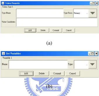
(24) 3.1. Edit Functions in OOMPNE. This section describes how the elements of an OOMPNet are created and edited in OOMPNE. In OOMPNE, there are five types of edit activties: 1. Insert and Delete 2. Copy and Paste 3. Move 4. Naming the Element 5. Decompose For example, the activities of type 1 are applied to create meaningful net elements in OOMPNE. The section introduces edit functions according to their element in the followings.. A. Color Set and Variables In the very beginning of constructing an OOMPNet, color sets and variables need to be created. The color sets and variables of an OOMPNet are also called declarations of an OOMPNet. Figure 3-2 shows the windows in editing color sets and variables. Window “Token Property” is used to define the color set for describing the type and value of tokens. When user creates a complex type of color set, OOMPNE creates a new sheet for user to model the object-net corresponding to the type. An object-net is defined with an OOMPNet. However, a token here is dynamic, i.e., the tokens inside the OOMPNet represented by their token might be changed dynamically. I.e., different inscriptions between an object-net and its type are the initial marking and the label of elements. The other inscriptions cannot be modified. User can use operation “Delete” to delete the color sets. Operation “Delete” pops out a list for user 15.

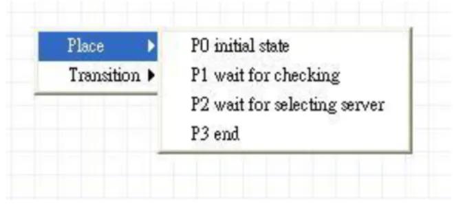
(25) to select and delete the color sets. The window “Set Variables” is used to edit he/she wants variables in OOMPNets. These variables are used to edit the inscriptions of arcs or transitions. The steps of operation “Delete” in function “Set Variables” are similar to that in function “Token Property”. It also provides a list for users to select and delete the variables.. (a). (b) Figure 3-2 The windows in editing token properties and variables.. B. Place Associated with a place, user can enter some special key to do the characteristics he wants. Or, he can popup a menu as in Figure 3-3 to help do the work. 1. Insert and Delete: The steps of creating places are described as follows. First, user selects the function “Add a place” in the drawing tool buttons. Second, user uses mouse to decide the position within the sheet. A place is now created into an OOMPNet. Then, user can edit the inscriptions of a place by using the operations in the popup menu associated with the place. In the menu, the first operation “Delete”, used to delete the target place. The rest operations will be introduced later. 16.

(26) Figure 3-3 The popup menu of right click a place.. 2. Copy and Paste: A use case can be divided into several usage scenarios. Usually, an action may be defined in more than one scenario. In order to create a share node fast, OOMPNE provides users the facility of duplicating existing nodes. Figure 3-4 shows the popup menu of duplicating operations, where the menu can be popped and each case in the menu corresponds to a distinct operation. The list shows the labels of existing places. User selects an element of the list to create the node with the same label. The operation of duplicating is to create an element with the same element type and label. Because an inscription is distinct in different scenarios, operation “duplicate” in OOMPNE does not duplicate the inscription(s).. Figure 3-4 The popup menu of operation duplicate.. 17.

(27) 3. Naming the elements: OOMPNE provides initial name, i.e. P0, P1, …, of new created places. The operation “Edit Label” in the popup menu in Figure 3-3 is used to edit the label of the place. 4. Decompose: “Set Abstraction” in the popup menu, shown in Figure 3-3, is in charge of decomposing places. “Set Abstraction” can be used to refine the place. When an abstract place is generated, the refinement is started by applying “Set Abstraction”. “Cancel Abstraction” is used to change the level of a place from abstract to primary.. C. Transition There is an associated popup menu in Figure 3-5. The operations of editing inscriptions of a transition are in the menu. These operations are introduced in the followings. 1. Insert and Delete: The steps of creating transitions are similar to those of creating places. The following introduces how to edit the inscriptions of a transition directly. The operations in the popup menu of transitions are: delete, edit label, set or cancel abstraction, set condition, show detail, set synchronization and rotate. Operation “Set Condition” is used to edit the guard expression(s) of a transition. On the other hand, user can use “Show Detail” to review the edited guard expression(s) of the transition. During a review, if user finds an error in the guard expression(s), he can use “Set Condition” to correct the guard expression(s). A synchronization relationship between transitions is constructed by using “Set Synchronization” operation. “Set Synchronization” provides user all transitions in corresponding 18.

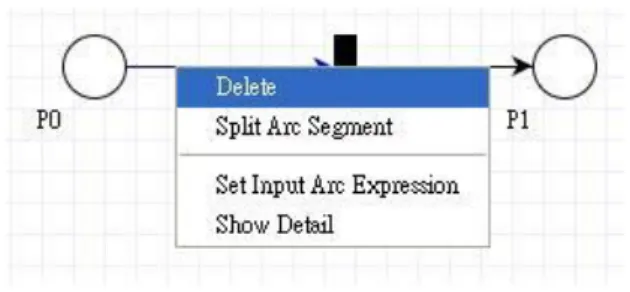
(28) object-nets to select the synchronous transition(s). Operation “Rotate” has three candidates, 45, 90 and -45. It is used to change the angle of a transition. The operation “Delete” is similar to that in popup menu of places. Transitions can be deleted through operation “Delete” or the “delete” key in keyboard.. Figure 3-5 The popup menu of a transition.. 2. Copy and Paste: In Figure 3-4, operation “duplicate” provides duplicating transitions. The steps of duplicating transitions are similar to the work for places. 3. Naming the elements: OOMPNE provides initial name, i.e. T0, T1, …, of new created transitions. The operation “Edit label” in the menu is used to edit the label of a transition. 4. Decompose: “Set Abstraction” in the popup menu, shown in Figure 3-5, is in charge of decomposing transitions. “Set Abstraction” can be used to refine the transition. The operation in transitions is similar to that in places. Here omits the detail of the operation.. D. Arc Figure 3-6 shows the popup menu associated with an arc. The operations displayed in 19.

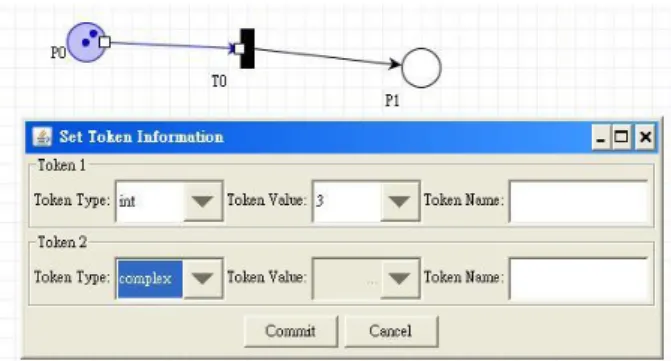
(29) such a popup menu include: delete, split arc segment, set input arc expression and show detail. 1. Insert and Delete: Creating an arc basically include the following 3 steps: 1) selecting the “Add an arc” function in drawing tool buttons, 2) using mouse to click an element to be the source of the created arc, and 3) click another element to be the destination of the created arc. There two popup menus associated with the arc, one for the arc whose destination is a place and the other for transition. In OOMPNE, the arc is called input arc if the destination is transition; otherwise the arc is called output arc. Operation “Delete” is used to delete the target arc. An arc might cross other elements in complex models. User can create turning point to mitigate the crossing situation by using operation “Split Arc Segment” in the popup menu. “Set Input Arc Expression” is used to edit the arc expression of the targeted input arc, similarly, “Set Output Arc Expression” is used to edit the arc expression of the targeted output arc. User can review the edited arc expression by using “Show Detail” in the popup menu to help finding out error(s) to be fixed.. Figure 3-6 The popup menu of an input arc.. E. Token The operations associated with tokens are list in popup menu in Figure 3-3. They contains: edit token, set token information and show detail. 20.

(30) 1. Insert and Delete: User can apply the function of “Add a token” in drawing tool buttons, shown in Figure3-1. Then, he can click a place to add the token into the place. Now, the token is not defined complete yet. A token has to be added necessary inscriptions e.g. token type and token value. The work has to be done with the popup menu. Operation “Edit tokens” is another way to add or delete tokens. Deleting tokens is also achieved by using function “Delete a token” in the drawing tool buttons. The steps in “Delete a token” are similar to that in “Add a token” function. Operation “Set token information” is used to edit the inscriptions of tokens. After editing the inscriptions of tokens, user can use “Show Detail” operation to review the inscriptions of tokens. During review, user can use “Set token information” operation again to modify the inscriptions of tokens to fix his problem. 2. Naming the element: In OOMPNets, complex tokens are named for representing the object-nets. It is easy to describe the marking of OOMPNets. The naming operation is associated with operation “Set token information”. Figure 3-7 shows the window to edit.. Figure 3-7 The window in editing tokens.. 3. Decompose: After editing the inscriptions of tokens, OOMPNE can be applied to open a sheet 21.

(31) for user to model the object-net for a token whose type is complex. The newly created sheets are already filled in the duplication of the type object-net. User can modify the object-net to fit condition(s). It reduces the time of modeling object-nets.. 3.2. Basic Abnormal Phenomena. There might be some abnormal phenomenon after an editing activity. In this section, we present the basic abnormal phenomenon right after an editing activity of modification, including “create” and “delete”. The anomalies corresponding to the activities in previous section are illustrated and discussed below:. A. Color Set and Variables The deletion of a color set or a variable might cause a problem, loss meaning. Loss meaning means that user edits an inscription of a net element with undefined types, values or variables. For tokens, a token with deleted type cannot be removed by the corresponding arc expressions. It remains in the initial place at run time. For arcs, arc expressions with deleted data cannot consume or produce the token from or to corresponding place(s) at run time.. B. Place and Transition (1) An arc cannot exist without source or destination. The deletion of a place or transition causes the associated arc(s) to lose source or destination. (2) The label of share nodes is different. A place or transition is called a share node if at least one place or transition with the same label in other OOMPNets. 22.

(32) The label of share nodes is different when the label of a share node is changed.. C. Arc The edition of an arc might cause some abnormal phenomena, as follows: (1) An arc connects two nodes with the same type in OOMPNets. From the definition of OOMPNets, an arc cannot be positioned between the same type elements. In other words, the source and destination of an arc cannot both be places or transitions. (2) A defined arc expression is combined with one or more undefined variables. It causes the corresponding transition to be fired impossibly. (3) Unbalance arc expression is an abnormal phenomenon which causes tokens to be remained in a place or an unfirable transition. The edition of an arc expression might cause “unbalance arc expression”. There are two situations to be concerned in the following: 1) For a place p, the union of its input arc expressions exp rsin does not combine with a token type which is defined in the union of output arc expressions exp rsout .. s  C( p ) : the value of coefficient n of s is 0 in exp rsin , the value of coefficient n' of s is greater than 0 in exp rsout . During run time, firing the transitions connected with input arcs does not add any token of type s into place p. However, without the token, some transitions of the output arcs cannot be fired later. Because the tokens in p cannot satisfy with the expressions of some output arcs, the transitions of the unsatisfied output arcs are not firable even if the guard expressions of 23.

(33) these transitions are satisfied. The unfirable circumstances could spread to the connected transitions arrowed. 2) For a place, the union of its input arc expressions exp rsin combines with a token type which is not defined in the union of output arc expressions. exp rsout . s  C( p ) : the value of coefficient n of s is greater than 0 in exp rsin , the value of coefficient n' of s is 0 in exp rsout . At the run time, a transition does not consume the tokens typed with s from place p added by input arcs. These tokens remain in place p. A large number of tokens remained in p could result in memory overhead that happens depending on the execution time of the transitions which add token of type s to p. (4) The deletion of an arc might cause some unbalance arc expression(s). Each arc deletion might cause exp rsin or exp rsout to change. So, unbalance arc expressions might be caused by deleting arcs.. D. Token (1) The tokens are positioned everywhere within a sheet without associated with places. Tokens cannot be positioned freely within a sheet. From the definition of OOMPNets, it is meaningless if a token is not put inside a place in an OOMPNet. (2) Users might use undefined types or values to edit the inscriptions of tokens. It causes the token to be unconsumable, because the corresponding arc expressions are not combined with the undefined type. (3) In an OOMPNet, a complex token has to be named necessarily. Naming a 24.

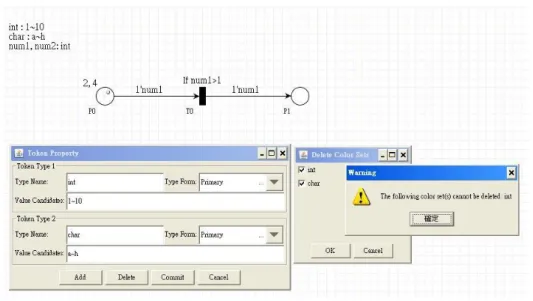
(34) primary token is unnecessary and then user is confused primary tokens with complex tokens.. 3.3. Incremental Analysis for the Anomalies in OOMPNE. The anomalies in previous section indicate some wrong net structures potentially. This section describes how OOMPNE reminds users to prevent those anomalies. The functions for preventing each anomalies are illustrated below:. A. Color Set To prevent loss meaning, OOMPNE checks the inscriptions of all net elements in OOMPNets whenever user deletes token type(s). OOMPNE uses message to remind user that the deletion causes some meaning loss. Figure 3-8 shows the message of deleting types, int and char. Type int is used in the OOMPNet. The message shows that type int cannot be deleted.. Figure 3-8 The reaction from OOMPNE of deleting used color set(s).. 25.

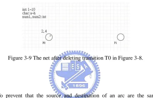
(35) B. Place and Transition (1) To prevent an arc without source or destination, OOMPNE deletes the arc(s) connected to the deleted place or transition directly. Figure 3-9 shows the net after deleting transition T0 in Figure 3-8. (2) When user changes the label of a share node, OOMPNE synchronizes the label of the share nodes in the other OOMPNets.. Figure 3-9 The net after deleting transition T0 in Figure 3-8.. C. Arc (1) To prevent that the source and destination of an arc are the same type, OOMPNE changes the destination point into turning point directly. Figure 3-9(a) shows the destination changed into turning point behind place P1. Figure 3-9(b) shows the turning point by moving place P1.. (a). (b). Figure 3-10 (a) the destination changed into turning point when user connects two places. (b) the turning point is shown by moving place P1. 26.

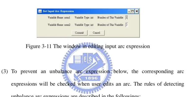
(36) (2) OOMPNE provides a defined variable list for user to edit arc expressions. Each variable in the list is associated with a blank space to be filled in an integer representing the limitation for the corresponding variable when the transition is fired. It prevents that user uses undefined variables to edit arc expressions. Figure 3-10 shows the window in editing input arc expressions from Figure 3-8.. Figure 3-11 The window in editing input arc expression. (3) To prevent an unbalance arc expression below, the corresponding arc expressions will be checked when user edits an arc. The rules of detecting unbalance arc expressions are described in the followings: N : F  ( P  T )  ( T  P ),N is a node function. The node function maps each arc int o a pair where the first element is the source node and the sec ond the destination node. IA,OA : P  T  F *. IA( p )  { f  F | t  T ,N( f )  ( t, p )},IA( p ) is a set of input arcs of place p OA( p )  { f  F | t  T ,N( f )  ( p,t )},OA( p ) is a set of output arcs of place p. Var : ( F  T )  Variables,Var( e )  { v Variables | v is used in A( e ) or G( e )} Type :Variables   ,Type( v )  { t   | the type of v is t }. Rule1 : p  P,If IA( p )   and OA( p )  , then.  . Type( v ) . fi IA( p ) vVar( fi ). Rule2 : p  P,If IA( p )   and OA( p )  , then. . . fo OA( p ) vVar( fo ). 27.  . Type( v )  C( p ). fo OA( p ) vVar( fo ). Type( v )  C( p ).

(37) Rule3 : p  P,If IA( p )   and OA( p )  , then.  . Type( v )  C( p ). fi IA( p ) vVar( fi ). The unbalance arc expression will be checked when user deletes an arc or edits the expression of an arc. The action of editing the expression(s) of an arc or deleting an input arc could cause the problem of case 1) in section 3.2. The action of editing expression(s) of an arc or deleting an output arc could cause the problem of case 2) in section 3.2. When an edition violates above rules, OOMPNE reminds user with a corresponding message. Figure 3-11(a) shows the message of editing an arc expression which causes an unbalance arc expression. The message of user’s deleting action which causes an unbalance arc expression is shown in Figure 3-11(b).. (a) edit expression of arc (P1,T1). (b) delete arc (T0,P1) Figure 3-12 (a) and (b) show the reminding ways of OOMPNE when user’s action violates the rules.. 28.

(38) D. Token (1) The tokens are associated with places. There are two ways to create a token: 1) perform operation “Edit Tokens” in the menu associated with place and 2) perform the function “Add a token” in drawing tool buttons. The action of adding tokens through “Add a token” is valid when the clicked element is a place. The two ways of creating tokens ensure that the created token is put in places. (2) Figure 3-8 shows the window in editing the inscriptions of a token. The combo selection of token type provides the pre-defined types for user to select. After selecting a type, the combo selection of token value provides the corresponding value candidates for user to select. Token name is unable to be filled in if the selected type is primary type. From the above functions, OOMPNE avoids using undefined token types to edit inscriptions of tokens and naming a primary token.. 29.

(39) Chapter 4. Technology of Analyzing OOMPNets. In order to analyze OOMPNets, this chapter provides algorithms to transform OOMPNets into CPNs. The CPN transformed from an OOMPNet is called T-CPN. Our algorithm merges object-nets with system-net recursively till the T-CPN is generated. During the transformation, the hierarchical relationship between object-nets and system-nets are maintained in a table for indexing. The names assigned for the token types, complex tokens and variables included in the OOMPNet are unique. The mechanisms adopted in our algorithms are introduced in section 4.1. The details of the algorithms proposed in this thesis are illustrated in section 4.2.. 4.1. The Mechanisms of Transformation Algorithms. The mechanisms adopted for implementing the algorithms proposed in this thesis can be separated into two parts: unfolding abstract node and generating transition. The definitions and functions included in the two parts are introduced one by one. In our methodology, all the abstract nodes of a system-net are unfolded before transformation. The transformation algorithms operate a system-net unfolded with its object-nets which have primary tokens only. The transitions of transformation result are generated by referring SRs on the condition. The functions offered for unfolding abstract nodes are established as follows: Function 4-1 (Unfolding an Abstract Place of an OOMPNet) : Let an OOMPNet N  (, P, T , D, F , C , G, A, I , L) be defined with an abstract place p whose refinement is rPNet  (' , P' , T ' , D' , F ' , C' , G' , A' , I ' , L' ) . The result of. 30.

(40)            unfolding p of N with rPNet is N  (, P, T , D, F , C, G, A, I , L) , where:.  ' (1)      is the union of two sets of types (colour sets) which belongs to net N and p’s refinement, respectively.. . (2) P  P  P' \{ p} contains all places of P and P ' except the abstract places p .  ' (3) T  T  T is the union of two sets of transitions which belongs to net N and p’s. refinement, respectively.  (4) D  D  D ' is the union of two sets of tokens which belongs to net N and p’s. refinement, respectively.   (5) The directed arcs of N are enumerated in set F which is consist of the two parts: (1) the first part holds the arcs contained in F and F’ except which exist between p and a transition or vice versa and (2) the second part includes the arcs connecting the input transitions of p to the places of P ' and the places of P ' to the output transitions of p.  F  F  F ' \ {(n1, n2 )  F | n1  p  n2  p}  {(t , pin ) | (t , p)  F , t  T , pin  P '}  {( pout , t ) | ( p, t )  F , t  T , pout  P '}       C ( p) (6) The color function C is defined from P to D . p  P, C ( p )   ' C ( p) (7) The. guard.  function G maps.    G (t ) t  T , G (t )   ' G (t ). each transition. ,if t  T ,if t  T '. 31. to. ,if p  P ,if p  P '. boolean expression..

(41)  A( f )    A' ( f )    (8) f  F , A( f )     A( f ' )  . , if f  F , if f  F '  , if N ( f )  (t , pin )  N ( f )  ( pout , t ), t  T f '  F , N ( f ' )  (t , p)  N ( f ' )  ( p, t ).    (9) The initialization function I is defined from P into expressions with tokens in D ..    I ( p) p  P, I ( p )   '  I ( p) (10) The. level. function.     L ( n) n  P  T , L (n)   '  L ( n). , if p  P , if p  P '.  L. is. defined. from.   P T. into. levels.. ,if n  P  T ,if n  P '  T '. Function 4-2 (Unfolding abstract transition) : Let an OOMPNet, O  (,V , P, T , D, F , C , G, A, I , L) with an abstract transition t, and the refinement is rTNet  (' ,V ' , P' , T ' , D' , F ' , C' , G' , A' , I ' , L' ) . Then we define.             the unfolded N to be O  (,V , P, T , D, F , C, G, A, I , L) where:  (1)     ' is the union of two sets of types (color sets) which belongs to net O and t’s refinement, respectively.  (2) V  V  V ' is the union of two sets of variables which belongs to net O and t’s. refinement, respectively.  (3) P  P  P ' is the union of two sets of places which belongs to net O and t’s. refinement, respectively..  (4) T  T  T ' \{t} contains all transitions of T and T’ expect the abstract transition t. 32.

(42)  (5) D  D  D ' is the union of two sets of tokens which belongs to net O and t’s. refinement, respectively.   (6) The directed arcs of O are enumerated in set F which is consist of the two. parts: (1) the first part holds the arcs contained in F and F’ except which exist between t and a place or vice versa and (2) the second part includes the arcs connecting the input places of t to the transitions of T’ and the transitions of T’ to the output places of t.  F  F  F '  {( p, tin ) | ( p, t )  F , p  P, tin  T '}  {(tout , p) | (t , p)  F , p  P, tout  T '} \{(n1 , n2 ) | n1  t  n2  t} (7) The. color. function.  C. is. defined. from.  P. to.  D. ..    C ( p ) ,if p  P p  P, C ( p )   ' ' C ( p ) ,if p  P  (8) The guard function G maps each transition to boolean expression..    G (t ) t  T , G (t )   ' G (t )  A( f )    A' ( f )    (9) f  F , A( f )     A( f ' )  . ,if t  T ,if t  T '. , if f  F , if f  F '  , if N ( f )  ( p, tin )  N ( f )  (tout , p), p  P f '  F , N ( f ' )  ( p, t )  N ( f ' )  (t , p).   (10) The initialization function I is defined from P into expressions with tokens  in D ..    I ( p) p  P, I ( p )   '  I ( p). , if p  P , if p  P '.    (11) The label function L is defined from P  T into labels.. 33.

(43)     L( n) n  P  T , L (n)   '  L ( n). ,if n  P  T ,if n  P '  T '. In addition, for the complex token(s) located in the input place(s) of transition t, the binding function bct of t (defined in Definition 4-1) selects a set of complex tokens from t’s input places for consuming. The notations used for defining bct are introduced here: (1) n  P  T : S (n)  { f  F | n'  P  T :[ N ( f )  (n, n' )  N ( f )  (n' , n)]} Function S maps node n to the set of n’s incoming and outgoing arcs, i.e., n is at one of the end of these arcs. (2) t  T : Var (t )  {v | v Var (G(t ))  f  S (t ) : v Var ( A( f ))} The set of variables in the guard expression of transition t is denoted by Var (t ) . (3) t  T : CTVar (t )  Var (t ) \{v | v.type is prime} Set CTVar (t ) contains all variables typed with complex in Var (t ) .. Definition 4-1 (Complex Tokens Binding): A complex tokens binding of a transition t is a function bct defined on CTVar (t ) , such that: v  CTVar (t ) : bct (v)  Type(v). we denote the set of all complex tokens bindings for t by BCT (t ) .. Complex. token. bindings. are. usually. written. in. the. form. ctv1  ct1, ctv2  ct2 ,..., ctvn  ctn where ctvi  CTVar  t  and cti COD , 1  i  n .. When an element ctvi  cti belongs to a binding generated by bct, we use. 34.

(44) ctvi  cti  bct to denote the relation. bct is used as ctv1  ct1,..., ctvn  ctn in the followings because, for each ctv1  ct1,..., ctvn  ctn , there is a corresponding binding function. The relationship is defined by the binding element given in Definition 4-2.. Definition 4-2 (Binding Element of Complex Tokens): A binding element of complex token(s) is a pair (t , bct ) where t T and bct  BCT (t ) . The set of all binding elements of complex tokens is denoted by. BECT .. An OOMPNet can be represented to a tree structure G  (V , E ) as the example neto shown in Figure 4-1. The case is applied for demonstrating the concepts proposed in the thesis. In the figure, a rectangle depicts a net and a directed arc connects two nets. The head of an arc is net ni.j located at the ith level and the tail is net ni-1.k located at one level higher which takes ni.j as a part. The node r having no superior is the root of the tree, denoted the system-net of the OOMPNet neto. The child nodes of r are object-nets, n2.1, n2.2 and n2.3, representing the complex tokens of r. A system-net holds the object-net(s) built by OOMPNets to be its complex token(s) and the complex token can be unfolded further to another system-net and object-net(s), e.g. n2.1 is a system-net of object-net n3.1 and n3.2. The belonging relationships are kept by the nets located in adjacent levels for all levels lower than r. Therefore, for all descendants of r, a net ni-1.k is a system-net of another net ni.j if ni-1.k is a parent node of ni.j in the hierarchy.. 35.

(45) level 1. r: system-net. net n2.1. net n3.1. net n2.2. level 2. net n2.3. level 3. net n3.2. .... .... .... ... net nm-1.1. level m-1. net nm.1. net nm.2. net nm.3. net nm.4. net nm.5. level m. Figure4-1 the hierarchical tree structure of an OOMPNet neto. The transformation algorithm provided in the thesis transforms an OOMPNet into a T-CPN by the bottom-up transformation procedure. The procedure traverses the tree of neto from leaves at the bottom to r at the top. One step progress of the transformation is proceeded by reconstructing the system-net ni-1.k with it object-nets ni.1,…,ni.n. The net obtained replaces the sub-tree depicted for ni-1.k and ni.1,…,ni.n. The four operations: (1) combining the variables and color sets belonging to ni-1.k and ni.1,…,ni.n, (2) duplicating the places and tokens of ni.1,…,ni.n into ni-1.k, (3) generating transitions based on the complex token bindings and the synchronization relationship(s) of ni-1.k and (4) connecting the nodes generated in (2) and (3) by arcs according to net ni-1.k and ni.1,…,ni.n are performed for accomplishing the reconstruction.. The concept of the algorithm moves the object-nets into the corresponding 36.

(46) system-net. So, the first two steps of the transformation algorithm collect the color sets, variables, tokens and places of the object-nets. Then, these elements are putted into the corresponding system-net directly. Before transformation, the complex tokens in system-net reference to object-nets respectively. After the two steps, a complex token references to the transformed places corresponding to the object-net which is referenced by the complex token before. It is because that the marking of object-net is also needed in T-CPN when builds occurrence graph.. In order to maintain the behaviors of OOMPNets in T-CPN, the third step of transformation concerns about the BCT of each transition and SR set. Here, this chapter defines the term Synchronous Transition Groups (STG), as Definition 4-3. Each group in STG defines which transitions are merged together. Each synchronous transition group is a set of transition(s) represented by a new transition in T-CPN. The transformation of transitions has three activities: First, creating transitions corresponding to the elements of BECT from each transition in the transforming OOMPNet. Second, the algorithm bases on the transitions from BECT and SR set to construct the STG and create the transition(s) representing the group(s) in STG. Third, the algorithm deletes the transition(s) which is(are) not representing the group(s) in STG. In a transformation, each transition t in the system-net is replaced by the transitions of the corresponding elements in set BECT if the BCT (t ) is not empty. The guard expressions of a transition corresponding to BCT (t ) are the primary guard expressions of the transition t . Then, the algorithm bases on the BECT and SR set to collect which transitions are merged together. If the BCT (t ) is empty, the transition t is added into the T-CPN directly. If a transition in system-net has synchronization relationship with a transition in object-net, its BCT is not empty. The transition mergence is according to SR set and the bct of each element in BECT. For 37.

(47) example, a transition t ' in the object-net and a transition (t , bct ) are merged together if (t, t ' ) belongs to SR set and the bct contains the complex token representing the object-net in the system-net.. Definition 4-3 (Synchronous Transition Groups, STG): A set of transitions form a synchronous transition group iff they fulfill the follows: 1. If the transition’s BCT is empty or the transition in an object-net without SR with a transition in system-net, it constitutes a synchronous transition group of its own. 2. For each transition in a synchronous transition group has synchronization relation with another transition in the synchronous transition group. 3. Each synchronous transition group contains one transition from the system-net and the other transitions from object-nets which are contained in bct of the system-net transition are not grouped from the same transition. For example, an OOMPNet SN with two object-nets, ON1 and ON2, is shown in Figure 4-2. The SR of SN is ( SN : T 0, ON 1: T 0) . The BECT of the SN contains binding element ( SN : T 0,  ctv  ON1  ) and ( SN : T 0,  ctv  ON 2  ) . The synchronization transition set of SN :T 0 holding elements (( SN : T 0 , ctv  ON 1  ),ON 1 : T 0 ) and ( SN : T 0 , ctv  ON 2  ) is generated by the binding elements. Moreover, the STG set {( ON 2 : T 0 , )} generated for ON 2 : T 0 denotes that there is no complex token. consumed when the transition is fired.. If SN is an object-net of another OOMPNet USN and transition T0 of USN has a synchronization relation with SN:T0, the SRs of USN is adapted by the STG set of. SN :T 0 . Thus, the adaption results are (USN : T 0,(( SN : T 0,  ctv  ON 1 ), ON 1: T 0)) and (USN : T 0,( SN : T 0,  ctv  ON 2 )) . The synchronization relations are kept by this way during net transformation. 38.

(48) Figure.4-2. An OOMPNet SN contains two object-nets.. For each synchronous transition group, here defines the guard expression of the transition which represents the synchronous transition group. The synchronous guard function SGF is defined from the set of transition groups, STG, into boolean expressions: T  STG : G(t )\{ g  G(t )|Type( g ) is complex } SGF(T )   (  tT G (t )  i. ,if t in system - net and G is the guard function of system - net ,if t in the i th object - net and Gi is the guard function of ith object - net. The transformation of an arc is according to transitions and places in the T-CPN. Arcs in OOMPNet are duplicated, created or modified to ensure that the behavior of the T-CPN could be similar to its corresponding behavior in the OOMPNet. In order to maintain the guard expressions of transitions about object-nets, this chapter defines OOT-Property Arcs (OOTPA). The format of guard expression about object-nets is ctv  m where ctv is a complex type variable and m is a marking of the 39. ).

(49) corresponding object-net. During a transformation, OOTPA is created according to the marking(s) in the guard expression(s). OOT-Property arcs are created in pairs. For example, Figure 4-2 shows a transition SN:T0 has a complex guard expression ctv=(1;-). Because the marking (1;-) has empty part, the corresponding places can be omitted the OOT-Property arcs. There are four OOT-Property arcs, (ON1:P0,SN:T0), (SN:T0,ON1:P0), (ON2:P0,SN:T0) and (SN:T0,ON2:P0), existed in the T-CPN. (ON1:P0,SN:T0) and (SN:T0,ON1:P0) is a pair of OOT-Property arcs. Similarly, (ON2:P0,SN:T0) and (SN:T0,ON2:P0) is a pair of OOT-Property arcs. In this example, SN:T0 has synchronization relation with ON1:T0, so the arc (ON1:P0,SN:T0) is already existed in T-CPN before creating OOT-Property arcs. Here discusses the arc expression of OOT-Property arcs. The creation of arc expression(s) of OOT-Property arcs is called OOT-Property arc function (OOTPAF). It contains two situations: 1) The OOT-Property arc can be added into the T-CPN directly. 2) There is an arc existed in the position where is the OOT-Property arc created. In the situation 1), the arc expression of the arc is multi-set of the marking described in the guard expression corresponding to the place. For example, arc expression of OOT-Property arc (ON2:P0,SN:T0) and (SN:T0,ON2:P0) in T-CPN of Figure 4-2 is 1’1. In the situation 2), it can be separated into two kinds: i) the destination of the existed arc is a transition and ii) the destination of the existed arc is a place. The algorithm uses the existed arc to be an OOT-Property arc by modifying the arc expression(s). Concerning i), algorithm bases on the arc expression of the existed arc and the marking in the guard expression to edit the arc expression of pair OOT-Property arcs. The arc expression of the existed arc is changed into the multi-set of marking in the guard expression corresponding to the place. And, the arc expression(s) of the matched OOT-Property arc is a function. Input of the function is the multi-set of the original arc expression of the existed arc. The output of the function is subtracting the 40.

(50) multi-set of the original arc expression of the existed arc from the multi-set of the marking in the guard expression corresponding to the place. In Figure 4-2, the arc expressions of (ON1:P0,SN:T0) and (SN:T0,ON1:P0) are 1’1 and f(exp)=1’1-exp respectively. If the arc expression of OOT-Property arc is empty, the OOT-Property arc can be omitted. Concerning ii), the arc expression of the existed arc is adding the multi-set of the marking in the guard expression corresponding to the place and the original arc expression of the existed arc. And, the arc expression(s) of the matched OOT-Property arc is(are) the multi-set of the marking in the guard expression corresponding to the place.. Function 4-3 (2-levels OOMPNet transformed into CPN): Let an OOMPNet O  (,V , P, T , D, F , C , G, A, I , L) , where there is no abstract place or transition. A T-CPN.          T  Net  (,V , P, T , F , C, G, A, I ) generated by. transformation algorithm where: 1. If COD  ,then O is a Colored Petri Net..  1 1. The COD is empty, so there is no complex type color set.   .  1  2. There is no complex type variable existed in V. So, V  V .  1  3. There is no complex token, so the place set of objct-nets is empty. Then, P  P.  1  4. There is no complex token, so the transition set of objct-nets is empty. Then, T  T .  1  5. There is no complex token, so the arc set of objct-nets is empty. Then, F  F.     1  6. The input of C is the places in P. Because P  P, C  C.     1  7. The input of G is the transitions in T . Because T  T , G  G.     1  8. The input of A is the arcs in F. Because F  F , A  A. 41.

(51)     1  9. The input of I is the places in P. Because P  P, I  I .. 2. If COD  , and | COD | m,then. dci  COD, dci  (ci ,Vci , Pci , Tci , Dci , Fci , Nci , Cci , Gci , Aci , I ci ) and CODci         (. . i 1...m.  2  2. V  V  (.  ci ). V. i 1...m.  2  3. P  P  (. . i 1...m. ci. ). Pci ); i  1...m, P  Pci  .  2  4. T  STG.   2  5. F  {( f , t )  ( F . . i 1...m.   C ( p) 2  6. p  P, C ( p)   Cci ( p).   Fci )  T | t ( f )  t }  OOTPA. ,if p  P ,if p  Pci.  A( f ' )     2  7. f  ( f ' ,t )  F , A( f )   Aci ( f ' )  OOTPAF( f ). ,if f '  F ,if f '  Fci  OOTPA ,if f  OOTPA.   2  8. t T , G(t )  SGF (t ).    I ( p) 2  9. p  P, I ( p)    I ci ( p). 4.2. , if p  P , if p  Pci. Transformation Algorithm. An algorithm, named OOMPNetToCPN, for transforming an OOMPNet to a CPN is presented in this section. The algorithm involves three sub-algorithms, ProduceElement, CreateSTG and CreateTransition, sequentially to achieve its goal. The ProduceElement algorithm is utilized to duplicate elements of the original net to 42.

(52) result. The CreateSTG algorithm is used to generate synchronize transition set(s) for keeping the dependent relations between transitions. The CreateTransition algorithm is applied to create transition(s) according to the BCTs of the system-net and the synchronization transition sets generated by CreateSTG. Let OOMPNet N be a source net of a series of transformations. A hierarchical representation of N is G  (V , E ) . Depth-first search [11] is applied to traverse graph G. The OOMPNetToCPN algorithm is executed on object-net ni.j, ni , j V , and its system-net ni-1.k when the algorithm finishes examining ni.j's adjacent nodes. Let ni 1,k  (,V , P,T , D, F , N , C, G, A, I , L) and ni , j  COD . Algorithm 4.1: OOMPNetToCPN(OOMPNet oonet, HashMap hierarchy){ 1.. //Input: oonet=(Σ, P, T, D, F, N, C, G, A, I, L): an OOMPNets with complex tokens. 2.. //. 3.. //Output: net: 1-level OOMPNet. 4.. for each apNet∈oonet.P.AP.net{. hierarchy: a hashmap to store the hierarchical level of the transformed net. 5.. oonet = UnfoldAbstractPlaces(oonet, apNet);. 6.. }. 7.. for each atNet∈oonet.T.AT.net{. 8.. oonet = UnfoldAbstractTransitions(oonet, atNet);. 9.. }. 10.. //Unfolding all abstract places and transitions in oonet. 11.. if(oonet.D.COD.size > 0){. 12.. //oonet.D.COD.size means the complex token number of oonet. 13.. for each d∈oonet.D.COD {. 14.. //recursively transforms OOMPNets into T-CPNs. 15.. OOMPNet cpn = OOMPNetToCPN(d.net, hierarchic);. 16.. //integrate color sets, variables and places of object-net into correspond system-net. 17.. oonet = ProduceElement(oonet, cpn, d, hierarchic);. 18.. }. 19.. //create the BECT transitions into net. 20.. oonet=CreateTransition(oonet);. 21.. ArrayList STGroup = CreateSTG(oonet.T, oonet);. 22.. //the creation of synchronous transition groups is according to Def 4-3. 23.. ArrayList STGTransition = new ArrayList(); 43.

(53) 24.. //store the transitions correspond to each group in STGroup. 25.. for each g∈STGroup{. 26.. Transition newTransition = new Transition();. 27.. newTransition.stg = g;. 28.. oonet.addPlaceTransition(newTransition);. 29.. STGTransition.add(newTransition);. 30.. }. 31.. //collect arcs existed in object-nets of oonet. 32.. Arc[] F’ = new Arc[];. 33.. for each d∈oonet.D.COD{ F’ = F’∪d.net.F;. 34. 35.. }. 36.. for each stgt∈STGTransition{. 37.. for each t∈stgt.stg{. 38.. stgt.guardExpres = stgt.guardExpres ∧ t. guardExpres;. 39.. for each f∈oonet.F∪F’{. 40.. if(t(f)==t){. 41.. Arc newArc = new Arc();. 42.. if(f.source == t){. 43.. newArc.source = stgt;. 44.. newArc.target = p(f);. 45.. }. 46.. else{. 47.. newArc.source = p(f);. 48.. newArc.target = stgt;. 49.. }. 50.. newArc.expres = f.expres;. 51.. oonet.addArc(newArc);. 52.. }. 53.. }. 54.. }. 55.. //create the arcs of OOTPA. 56.. if(t∈T && (complex guard expressions of t is not empty)){. 57.. for each m∈M{. 58.. //M is the set of the markings in the complex guard expressions of t. 59.. OOMPNets on = getCorrespondObjectNet(m);. 60.. //getCorrespondObjectNet is used to find the object-net. 61.. //corresponds to the marking m 44.

(54) 62.. for each p∈on.pt.p{. 63.. if(m(p)!=null){. 64.. if((p,t)∉F && (t,p)∉F){. 65.. Arc newInputArc = new Arc();. 66.. Arc newOutputArc = new Arc();. 67.. newInputArc.addExpres(multi-set of M(p));. 68.. newOutputArc.addExpres(multi-set of M(p));. 69.. newInputArc.source = p;. 70.. newOutputArc.target = p;. 71.. newInputArc.target = stgt;. 72.. newOutputArc.source = stgt;. 73.. net1.addArc(newInputArc);. 74.. net1.addArc(newOutputArc);. 75.. }. 76.. else if(f==(p,t)∈F){. 77.. Arc newArc = new Arc();. 78.. newArc.addExpres(f(exp)= multi-set of M(p) – f.guardExpres);. 79.. newArc.source = t;. 80.. newArc.target = p;. 81.. f.guardExpres = null;. 82.. f.addExpres(multi-set of M(p));. 83.. net1.addArc(newArc);. 84.. }. 85.. else if(f=(t,p)∈F){. 86.. Arc newArc = new Arc();. 87.. newArc.addExpres(multi-set of M(p));. 88.. newArc.source = p;. 89.. newArc.target = t;. 90.. net1.addArc(newArc);. 91.. f.guardExpres = f.guardExpres+multi-set of M(p);. 92.. }. 93.. }. 94.. }. 95.. }. 96.. }. 97.. for each t∈oonet.T{. 98. 99.. if(t∉STGTransition){ oonet.deletePlaceTransition(t); 45.

(55) 100.. }. 101.. }. 102.. return oonet;. 103.. }. 104.. else if(oonet.D.COD.size == 0){. 105.. //oonet without complex token. 106.. return oonet;. 107.. }. 108. }. This algorithm is the main recursive algorithm to transform OOMPNets into T-CPN. Inputs of the algorithm are one OOMPNet and a hashmap which is an index table described in Sec. 4.1. 1-level OOMPNet is an output of the algorithm. The final output is a T-CPN conform the description in Sec. 4.1.. Lines 4 to 9 in the algorithm unfold the abstract nodes in the OOMPNet. Lines 11 to 107 separate the input OOMPNet into two situations according to the number of complex token. An OOMPNet is 1-level if its complex token number is 0. Lines 104 to 107 return the inputted OOMPNet which is 1-level originally. Lines 11 to 105 concern the number of complex token is bigger than 0. Lines 8 to 13 find out the object-net. which is 1-level OOMPNet. by calling itself. Then, function. ProduceElement in line 17 integrates the declarations, places and tokens of the object-net into its system-net. For a 2-level OOMPNet, the declarations, places and tokens of all object-nets are integrated into the system-net after the for-loop in line 13 to 18 finish. Then, lines 20 to 101 realize the third and forth steps in transformation. Lines 20 to 30 transform transitions and lines 31 to 101 transform arcs. Line 20 calls function CreateTransition for creating the transitions corresponding to BCT of all transitions in oonet and put these new created transitions into oonet. Lines 21 to 30, like STG described in Def. 4-3, create STG and transitions correspond to the group of 46.