國
立
交
通
大
學
機械工程學系
博
士
論
文
低熱值燃料應用於環型微渦輪引擎之
實驗分析與數值模擬
Experimental Investigations and Numerical Analyses of an
Annular Typed Micro Gas Turbine using Low-heating Value Fuels
研 究 生:楊竣翔
指導教授:陳俊勳 教授
低熱值燃料應用於環型微渦輪引擎之
實驗分析與數值模擬
Experimental Investigations and Numerical Analyses of an Annular Typed
Micro Gas Turbine using Low-heating Value Fuel
研 究 生:楊竣翔 Student:Chun-Hsiang Yang 指導教授:陳俊勳教授 Advisor:Prof. Chiun-Hsun Chen
國 立 交 通 大 學 機械工程學系
博 士 論 文
A Dissertation
Submitted to Department of Mechanical Engineering College of Engineering
National Chiao Tung University in Partial Fulfillment of the Requirements
for the Degree of Doctor of Philosophy
in
Mechanical Engineering
November 2009
Hsinchu, Taiwan, Republic of China
I
低熱值燃料應用於環型微渦輪引擎之
實驗分析與數值模擬
學生:楊竣翔 指導教授:陳俊勳教授
國立交通大學機械工程學系
摘要
為了嶄新的世代,要解決石化燃料短缺危機與符合環保規範減量二氧化 碳的生成,再生能源的利用與新興能源的開發已經成為政府極力發展的能 源政策,本論文透過數值模擬與實驗分析檢驗了低熱值燃料應用於擁有環 型燃燒室之微渦輪引擎的可行性,研究中使用已開發完成的燃油氣渦輪引 擎 MW54 作為載具,並將其以燃油為燃料的燃燒室重新改裝成為適合低熱 值生質能氣體燃料之微渦輪引擎燃燒系統, 本論文包含三個部份,第一部分,本論文透過實驗分析,了解低熱值燃 料應用於擁有環型燃燒室之微渦輪引擎所能產生的效能。首先為微渦輪引 擎架設相關的驅動與感測裝置來完成研究用測試平台。研究中使用不同比 例的 CO2混合甲烷做為實驗用的低熱值燃料,透過量測得到的數據來分析 與評估此引擎的效能。實驗結果顯示,微渦輪引擎最低可使用 60% 甲烷含 量的燃料來運轉,而使用 90% 甲烷燃料時,發電量在 85,000 轉時達到 170W,且 70% 甲烷燃料可在 60,000 轉達到 70W。當使用 60% 甲烷燃料II 時,微渦輪引擎所能產生之動力相當的低。微渦輪引擎的布雷登循環效率 與發電效率可透過實驗數據的計算得知,最高分別是 23% 與 10%。 第二部分為透過套裝軟體 CFD-ACE+的應用完成了環狀微渦輪引擎在 供應低熱值的燃料下,燃燒室襯孔對於燃燒室內熱流場的冷卻效應與環狀 微渦輪引擎內的燃燒行為之數值模擬。分析的內容包括環狀微渦輪引擎內 的流動特性、燃燒行為、熱傳導分析、化學反應與彼此之間的交互作用。 模擬的結果顯示從稀釋區進入的空氣充分的發揮冷卻的效用,而此燃燒室 的設計在使用低熱值燃料時,並不會在襯桶壁上產生熱點且排氣溫度都低 於排氣溫度的最大容許溫度 800°C。 第三部分為未來工作的先前研究,包括了微渦輪引擎的系統鑑別。透過 實驗收集整合的數據,可以幫助我們鑑別控制系統內模擬模型的參數,系 統鑑別的工作是未來設計控制系統時所必備的。本論文完成了一個使用再 生性生質氣體的分散式發電系統,本系統體積小、低成本、維修容易且適 合推廣於家庭用。
III
Experimental Investigations and Numerical Analyses of an
Annular Typed Micro Gas Turbine using Low-heating
Value Fuel
Student: Chun-Hsiang Yang Advisor: Prof. Chiun-Hsun Chen
Department of Mechanical Engineering National Chiao Tung University
ABSTRACT
The utilization of renewable energy and development of new energy sources are the present governmental energy policy to cope with the more and more stringent shortage of fossil fuels and environmental regulations for carbon dioxide reduction in the new century. This dissertation examines the practicability of low-heating value (LHV) fuel on an annular micro gas turbine (MGT) through experimental evaluations and numerical simulations. The MGT used in this study is MW-54, whose original fuel is liquid (Jet A1). Its fuel supply system was re-designed to use biogas fuel with LHV.
There are three parts in this dissertation. In the first part, experiments were completed to evaluate the combustion efficiency of an annular MGT while applying the LHV fuel. The corresponding sensors and actuators for the MGT were established to form our test stand. The methane was mixed with different ratio of CO2 to be our LHV fuel. The measured data indicating the engine
performance were analyzed and evaluated. Experimental results showed that the presented MGT system operated successfully under each tested condition when the minimum heating value of the simulated fuel was approximately 60% of
IV
pure methane. The power output was around 170W at 85,000 RPM as 90% CH4
with 10% CO2 was used and 70W at 60,000 RPM as 70% CH4 with 30% CO2
was used. When a critical limit of 60% CH4 was used, the power output was
extremely low. Furthermore, the best theoretical Brayton cycle efficiency and electric efficiency of the MGT were calculated as 23% and 10%, respectively.
Following the experiments, the corresponding simulations, aided by the commercial code CFD-ACE+, were carried out to investigate the cooling effect in a perforated combustion chamber and combustion behavior in an annular MGT when using LHV gas. The investigation was conducted to realize the characteristics of the flow, combustion, heat transfer, chemical reaction, and their interactions in an annular MGT. The results confirmed that the cool air flows through dilution holes on combustor liners were functioning fully and there were no hot spots occurred in the liners. In addition, the exhaust temperatures of combustion chamber were lower than 1073K when MGT was operated under different conditions.
Finally, the system identification of MGT was completed for future studies. The model identification process is prerequisite for controller design research in the near future. The measured data helped us identify the parameters of dynamic model in numerical simulation. This dissertation presents a novel distributed power supply system that can utilize renewable biogas. The completed micro biogas power supply system is small, low cost, easy to maintain and suited to household use.
V
誌
謝
感謝恩師陳俊勳教授的悉心指導與各位審查委員的寶貴意見,感謝求學 生涯中遇到的每一個人,你們帶給了我不同的成長與幫助,謝謝您。七年 前,受到蔡明祺老師的提攜,讓我踏上了研究之路,碩士班的研究生涯, 受馮榮豐老師的指導,讓我打好了研究所需的一切根基,也了解了學術界 的生態與運作模式,之後在教授們的推薦之下,進入了交通大學博士班, 加入了陳俊勳老師所領導的燃燒防火實驗室的研究團隊。 實驗室中遇到的每一個人,都帶給我不同的回憶並豐富了我的求學經 歷,無敵、振稼、蕭哥謝謝你們對共同研究目標的努力;高苑莊老師、大 達、文魁、文耀學長謝謝你們的鼓勵與建議;瑭原、阿貴、振忠、達叔、 季哥、DC、金輝、瑋琮與實驗室的每一位,謝謝你們構築了我故事中的點 點滴滴,謝謝不斷出現,但誌謝本就該充滿感謝之詞。 最後在此將本論文獻給支持我一切的父母、同為學位努力的二姐與我的 女友,謝謝你們。
VI
CONTENTS
摘要 ... i ABSTRACT ... iii 誌謝 ... v CONTENTS ... vi List of Tables ... ix List of Figures ... xi Nomenclature ... xii Chapter 1 Introduction ... 1 1.1 Motivation ... 1 1.2 Literature Review ... 3 1.2.1 Numerical simulation ... 31.2.2 Micro gas turbine ... 7
1.2.2 Micro gas turbine modeling ... 12
1.3 Scopes of the present study.. ... 14
Chapter 2 Experimental investigation ... 17
2.1 Briefing of the proposed micro gas turbine system... 17
2.1.1 Transmission System ... 18 2.1.2 Fuel supply ... 19 2.1.1 Start system ... 19 2.1.1 Lubrication ... 19 2.2 Experiment layout ... 20 2.3 Measurement instrumentation ... 20 2.3.1 Data Acquisition ... 20 2.3.2 Temperature measurement ... 22 2.3.3 Turbine RPM measurement ... 22
2.3.4 Fuel pressure measurement ... 22
VII
2.4 Test stand operating procedures ... 23
2.5 Parameters of tests ... 25
2.6 Uncertainty Analysis ... 25
2.6.1 The Asymmetric Uncertainties of Thermocouple ... 26
2.6.2 Uncertainty Analysis of mass flow controller ... 27
2.6.3 The Experimental Repeatability ... 27
Chapter 3 Numerical analyses ... 30
3.1 Domain descriptions ... 30
3.2 Governing equations ... 30
3.3 CFD-ACE+ software ... 36
3.4 Numerical method ... 36
3.5 Boundary conditions ... 36
3.5.1 The inlet boundary conditions ... 37
3.5.1.1 Air inlet boundary conditions of combustor ... 37
3.5.1.2 Fuel inlet boundary conditions of combustor ... 39
3.5.2 The outlet boundary conditions ... 40
3.5.3 The symmetry boundary conditions ... 40
3.5.4 The interface boundary conditions ... 40
3.5.5 Wall boundary conditions ... 40
3.6 Computational procedure of simulation ... 40
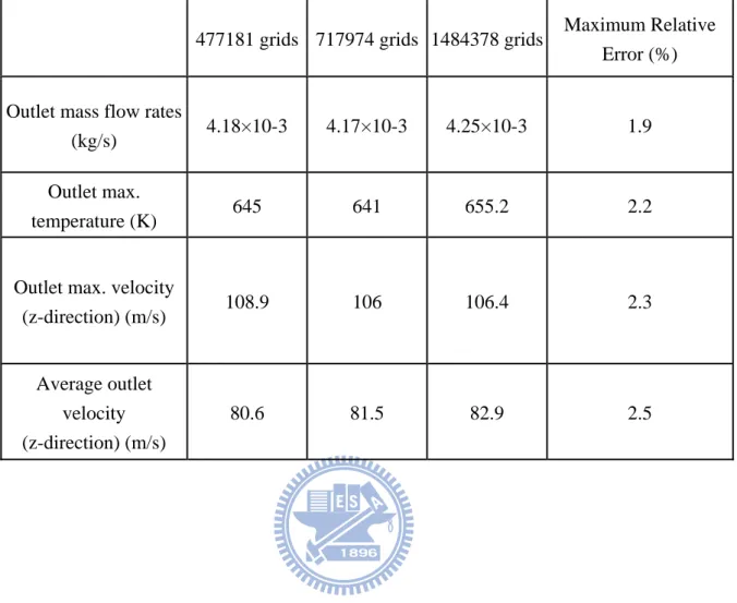
3.7 Grid-independence test ... 41
Chapter 4 Dynamic Model of MGT for Control Strategy ... 47
Chapter 5 Results and Discussions ... 49
5.1 Experimental results and discussions ... 49
5.1.1 Tests using various fuels with no load ... 49
5.1.1.1 Pressures and volume flow rates of fuel in the MGT ... 50
5.1.1.2 Temperature of unloaded MGT ... 52
5.1.1.3 Thermal efficiency ... 53
5.1.2 Testing MGT with generator ... 54
5.2 Numerical Simulation results and discussions ... 56
VIII
5.3.1 System identification ... 61
Chapter 6 Conclusions and Future Works ... 66
5.1 Conclusions ... 66
5.2 Future Works ... 67
ix
List of Tables
Table 2.1 Specifications of the data acquisition modules ... 21
Table 2.2 Experimental repeatability for volume flow rate for various fuels ... 29
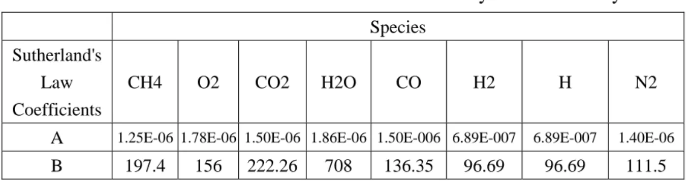
Table 3.1 Sutherland's law coefficients of dynamic viscosity ... 43
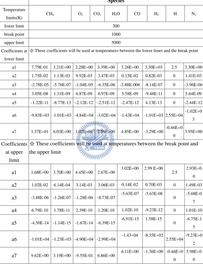
Table 3.2 JANNAF coefficients of gas specific heat ... 44
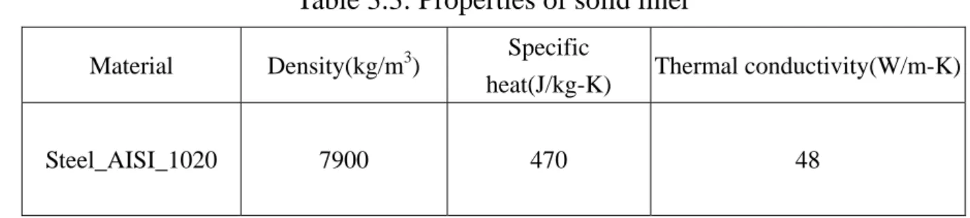
Table 3.3 Properties of solid liner ... 45
Table 3.4 Boundary conditions of combustion chamber ... 45
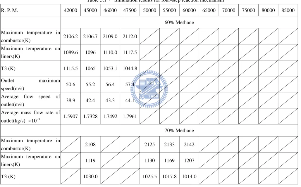
Table 3.5 Grid test results of different grid densities for numerical simulation 46 Table 4.1 Simulation results for four-step reaction mechanism ... 63
x
List of Figures
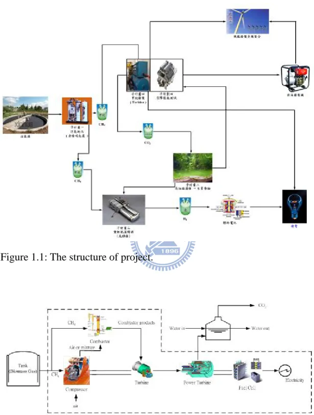
Fig. 1.1 The structure of project ... 73
Fig. 1.2 The basic structure of the MGT generator ... 73
Fig. 1.3 Pictures of the adopted micro gas turbine ... 74
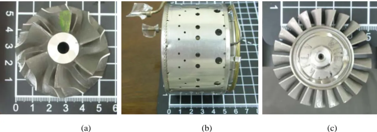
Fig. 2.1 Pictures of the major parts in MGT (a) Compressor; (b) Combustion chamber; (c) Turbine wheel ... 75
Fig. 2.2 Pictures of experimental facilities in proposed MGT system ... 75
Fig. 2.3 Schematic of experiment layout ... 76
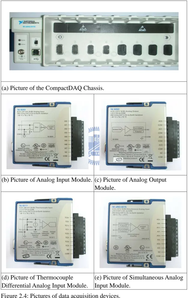
Fig. 2.4 Pictures of data acquisition devices ... 77
Fig. 2.5 Pictures of sensors and actuators for the proposed MGT system ... 78
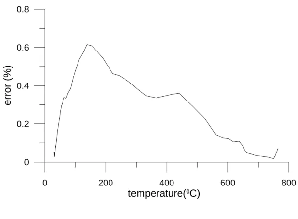
Fig. 2.6 The relationship of temperature and error ... 79
Fig. 2.7 Experimental error bars for CH4:CO2 mixing ratios ... 80
Fig. 3.1 The simplifying procedure of model domain illustrated by software Solid Works. ... 81
Fig. 3.2 The configurations of a sub-chamber ... 82
Fig. 3.3 The size specification of sub-chamber ... 82
Fig. 3.4 Grids generation for numerical computation ... 83
Fig. 4.1 Simulation model of micro gas turbine in SIMULINK ... 84
Fig. 5.1 Volume flow rate for fuels with LHV fuels at various RPMs ... 85
Fig. 5.2 Compressor speed vs. volume flow rate of CH4 with different concentrations of methane fuels ... 86
Fig. 5.3 Temperatures at different positions in the MGT (a) Fuel with 90% CH4; (b) Fuel with 80% CH4; (c) Fuel with 70% CH4; (d) Fuel with 60% CH4 ... 88
Fig. 5.4 (a) Combustion chamber (oil); (b) Combustion chamber using 70% CH4 (gas). ... 89
Fig. 5.5 Brayton cycle efficiency of different compressors speed with different concentrations of CH4 ... 90
Fig. 5.6 Output power for different generator rotation speeds with different LHV fuel. ... 91
Fig. 5.7 Simulation results of applying 60% methane fuel at rotation speed 45000RPM... 92 Fig. 5.8 Distribution of temperature for different concentration of methane at
xi
45000 RPM... 93 Fig. 5.9 Distributions of CH4 mass fraction for different concentration of
methane at 45000 RPM ... 94 Fig. 5.10 Distributions of O2 mass fraction for different concentration of
methane at 45000 RPM ... 95 Fig. 5.11 Velocity vector of flow field for different concentration of methane at 45000 RPM... 96 Fig. 5.12 Curved chart with different methane concentration and different compressor speed ... 97 Fig. 5.13 Maximum temperature at combustor outlet for different fuel ... 98 Fig. 5.14 Numerical result of output power for different generator rotation speeds with 90% CH4 ... 99
Fig. 5.15 Numerical result of turbine outlet temperature versus experimental time ... 100
xii
NOMENCLATURE
A Pre-exponential factor p C Specific heat h D Hydraulic diameter ih Enthalpy to different species 0
h Total enthalpy
I Turbulence intensity r
k Reaction rate constant
k k-equation for turbulent model m& Volume flow rate
i
m Mass flow rate to different species n Temperature exponent
p Pressure out
P Pressure of mass flow controller outlet L
Q Heat transferred out of the system H
Q Heat transferred into the system h
S Energy source
T Temperature
T1 Temperature of compressor inlet T2 Temperature of compressor outlet T3 Temperature of turbine inlet T4 Temperature of turbine outlet
u, v, w Velocity components in the (x, y, z) system of coordinates W Actual work of system
ρ Density
ij
τ Stress tensor component ε Dissipation rate
th
η The efficiency of standard Brayton cycle electric
1
Chapter 1
Introduction
1.1 Motivation
The greenhouse effect is an international problem. Controlling emissions of greenhouse gases is an important environmental goal. In response, the Taiwanese government has prioritized utilization of renewable energies and the development of new energy sources. As a large amount of biogas can be derived from bio-waste, this fuel source is currently favored in Taiwan. Marsh gas is comprised of approximately 50% methane. Although methane is lighter than both air and natural gas, it has similar thermal and physical properties. Methane generated from garbage, which is an air pollutant, can be used as fuel. Notably, generating electrical power using methane gas can reduce the emission of a greenhouse gas and simultaneously produce electrical power.
Recently, people pay intensive attention to find new sources of energy, to save energy, and to raise the consciousness of protecting environment. National Science Council has awarded our laboratory a three-year research project from 2006 to 2008. Fig. 1-1 shows the infrastructure of the project, which isdivided into four subprojects. The goal of the subproject 1 is to increase the utilization efficiency of biogas by removing H2S and improving the power generation rate.
The CO2 emitted from biogas will also be reduced by chemical methods. The
focus of the subproject 2 is to produce the biodiesel from high lipid-content algae in wasted CO2. The purpose of the subproject 3 is to develop a process
that may effectively produce hydrogen from primary products of biomass, including alcohols, methane of subproject 1, and biodiesel of subproject 2. The
2
subproject 4 develops a micro gas turbine (MGT) which could used to drive a
generator to produce the electricity by modifying the burner from a liquid-fuel burning gas turbine system into a gas-burning one to generate the combustion power. It is a co-generation process, which can be one of the potential candidates for the distributed power supply systems.
The research of this study focuses on subproject 4. The market assessments in 2000 identifies several potential types of power applications for MGT, including continuous generation, premium power, mechanical drive, and combined heat and power. Gas turbine is a system device supplying jet propulsion and/or power. Gas turbine can make the much stronger gas flows than a piston engine during the common continuous processes of running. The strength of gas flow can be changed to axial power by a gear box with a turbine. If the axis is connected to a generator, the gas turbine can be used to generate electric power.
MGTs offer a lot of potential advantages over other technologies for small-scale power generation. There are less moving parts in a MGT, so there would be less friction loss, lower vibrating, lower electricity costs, high reliability and less maintaining cost. Besides, the size of a MGT is smaller and its weight is lighter so it can generate a high power-to-weight ratio and lower emissions.
It can be located on sites with limited space to produce power, and the waste heat recovery can be used to improve more than 80% efficiencies. Compared with the reciprocating engine, MGT is also more efficient because of its simple structure and less moving parts. In terms of power density, gas turbine is also better than the reciprocating engine. Combining the MGT with the methane gas could generate electric power, and the methane gas could replace the traditional
3
oil fuel.
The methane gas is obtained from the purified marsh gas through bio-process. Owing to the limitation of present biochemical technique, there still exists a little amount of impurity gases, such as carbon dioxide (CO2), which
cannot be removed completely. It would dilute the concentration of pure methane gas so that the MGT is not easily to operate.
In addition to the concern of heat value, the phase state of liquid is different from that of gas. This difference would cause the mismatch of the gas turbine system. The components of gas turbine can be roughly divided into three parts: compressor, turbine wheel and combustion chamber. With introducing the low heating value (LHV) fuel, its total mass flow has a much greater mass fraction of air than that with a liquid fuel. Consequently, the reaction behaviors in combustion chamber are also changed. Therefore, the gas turbine should be adjusted to be able to apply LHV fuel. When the system is microminiaturized, it can be used in many kinds of electric power demands, such as electric vehicles, motorcycles, portable generators, and even PCs and laptops.
1.2 Literature Review
1.2.1 Numerical simulation
Much previous research on micro gas-turbine had made effort to improve the combustor efficiency or to bring up novel designs. Most design factors and coefficients were obtained from experiments and designers’ experience. Especially, the combustion chamber is the most heavily thermal load part in a turbine engine and its service life is normally very short. Since very limited data can be obtained from expensive engine tests due to its serious work environment,
4
a well founded numerical simulation will lower the process cost between design and experiment layout.
As powerful computing technologies are continuously and rapidly improved, computational fluid dynamics (CFD) methods have become a feasible tool in the aero-turbine industry. Many of the previous CFD models of gas turbine combustors included only calculation of reacting flows within the combustor liner while assuming profiles at the various liner inlets [1-5].
Lawson [1] calculated the reacting flow inside the combustor liner. A structured single-block grid was used in this study. Lawson was able to successfully match the calculated radial temperature profile at the combustor exit with experimental data, and then used the calibrated CFD model to predict the radial temperature profile that resulted from different cooling and dilution air patterns. Lawson used a one-dimensional code to predict flow splits, and a two-dimensional CFD model to predict the flow profile at the exit plane of the swirl cup. This profile was then applied as a boundary condition in the 3D model.
Fuller and Smith [2] predicted the exit temperature profiles of an annular direct flow combustor that were in fairly good agreement with measurements. They used a structured multi-block grid in their calculations, which was essential for modeling complex geometries. They also used a two-dimensional model to provide the boundary conditions at the exit plane of the swirl nozzle.
Gulati et al. [3] devoted to study a 3 dimensional full-scale 10-cup combustion sector with double-annular. Calculations were carried out for the same geometry and operating conditions using the CONCERT-3D CFD code. A single block structured grid was used to calculate the flow inside the combustor liner. The predicted exit plane mean and RMS temperature, and mole fraction of the major species were then compared with the measured data, and were found to
5
be in fair agreement. The effects of various inner/outer dilution air jets combinations on the exit plane mean temperature (radial distribution of the circumferentially averaged temperature) and major species mole fractions were also studied and compared with the experimental results. The calculated results were found to recover the trends of these geometry variations fairly well.
Danis et al [4] used the proprietary code CONCERT to calculate the inner chamber flow of five modern turbo-propulsion engine combustors. The N-S equations were solved for turbulent reacting flows, including spray modeling. The 3D CFD models were first calibrated based on design database for one combustor. The anchored models were then run successfully for the other four combustors. A structured single-block grid was used in this research with suitable meshing around the internal obstacles. Two-dimensional results for the exit velocity profiles, along with measured spray quality, were used as a swirl cup inlet condition for the 3D calculations. Consequently, the turbulence properties at the swirl cup in the 3D calculations were calibrated using design database.
Lai [5] modeled the inner chamber of a gas turbine combustor similar to that of the Allison 570KF turbine used by the Canadian Navy. A 22.5 deg periodic sector of the combustor was modeled using a structured multi-block grid. Lai included the swirled passages in his model, which was an important step in reducing the uncertainty in the boundary conditions. The simulation results for the combustor flow fields in this research didn’t compare with the experimental data.
In a recent study, Gosselin et al. [6] simulated steady, 3D turbulent reacting flows with liquid spray, in a generic type gas turbine combustor using a hybrid structured/unstructured multi-block grid. The commercial FLUENT code was used in this study. The calculation allowed for detailed combustor geometry, including the inner chamber, external channel, and the various liner film cooling
6
holes and dilution ports. The N-S equations were solved using the k-_/RNG turbulence model and the PDF turbulent kinetic energy reaction rate model. The calculated results for the gas temperatures, mass functions of CO/CO2, and
velocity fields were compared with experimental measurements. However, no prediction of the wall temperature was included in this work.
Ho et al. [7] proposed a prototype simulation modeling of annular combustor chamber with two-phase flow field. Ho’s research utilized the commercial code, INTERN, which was developed and technically supported by NERC.
Crocker et al. [8] used a software CFD-ACE to simulate a combustor model from compressor diffuser exit to turbine inlet. Their model included an air-blast fuel nozzle, dome, and liner walls with dilution holes and cooling louvers. The comprehensive model made it possible to predict flow splits for the various openings into the combustor liner and to remove the guesswork required for prescribing accurate boundary conditions for those openings. The simulation was combining the conjugate heat transfer analysis and the gas radiation. The coupled modeling which could provided a direct prediction of liner wall temperatures including both inside and outside the liners. Non-luminous gas radiation added approximately 40K to the hot side of metal wall temperature.
Priddin and Eccles [9] also demonstrated the capability of full-combustor structured-mesh analysis, and highlighted the usefulness of a streamlined CAD-to-grid process utilizing parametric solid models. Birkby et al. [10] developed a description of an analysis of an entire industrial gas turbine combustor, in which the premixing fuel nozzle was coupled with the combustion chamber. Snyder and Stewart [11] developed a CFD analysis on an entire PW6000 combustor domain to predict temperature distribution at the combustor exit and compared the CFD result with the full annular rig-test data.
7
However, all aforementioned studies on “full combustor” omitted cooling devices or simplified cooling holes to slots.
Li et al. [12] proposed a fluid-solid coupling simulation in an aero-engine annular combustor to investigate the integrated contribution of combustion and cooling to the thermal load in a completely structure annular tube. The reliability of the simulation was demonstrated by comparing calculated combustor exit temperature distributions with profiles of the rig-test measurements. The predicted profile was in a quite good agreement with the rig-test data indicating that the proposed CFD analysis could explore the major performance of the fluid flow and combustion in the gas turbine combustor. The simulation results showed that the combination of local combustion and shortage of coolant might lead to film cooling/protection failure in some regions of the combustor.
1.2.2 Micro gas turbine
Wen [13] studied the micro turbine generator system that introduced the experimental foundation for a 375hp micro turbine generator system, which included inlet and exhaust section, testing frame, operating control system and measurement system. Besides, the operating control systems of the micro turbine generator system that included starter system, fuel supply system, lubrication system, ignition system and secondary air supply system of combustor had to be set up. Additionally, the measurement devices and data acquisition system needed to measure the engine baseline performance were completely designed and constructed.
Wang [14] tested and analyzed a 150 kW micro turbine generator set with twin rotating disk regenerators. Using the PC-based data acquisition system, the engine speed, turbine inlet temperature, exhaust temperature, compressor inlet
8
and discharge pressure, and fuel flow rate were all measured. The generator set was tested by using load bank to establish the baseline performance including temperature, pressure, horsepower, fuel consumption, and speed. He used the software program GasTurb to predict the performance of the micro turbine generator set in different operating conditions in order to compare with the test results. The thermal efficiency of 28% was predicted at full load with regeneration while the no regeneration case only had 14% thermal efficiency.
There are a few companies currently working on micro-turbines in the 25-250 KW range. To understand the state of industry, a brief overview of some of the companies and their products are discussed. The name “Capstone” [15] often arises in conversations about micro-turbine generators. One of their smaller generators is a 30 KW load-following device that is set up for combined heat and power (CHP). The device is 26% electrically efficient and boasts one moving part, namely the compressor-turbine-generator shaft. From the heating and cooling end, the unit emits 85 KW of thermal energy that can be used to power an absorption chiller or heat exchanger. One major advantage of this device is that it is a relatively quiet machine, which operates at 65 db when it is measured 10 m away. Capstone has also developed a large 65 KW device that is 29% electrically efficient and outputs 78 KW of thermal energy for CHP applications. It has a total fuel efficiency of 64%.
Bowman Power [16] has an 80 KW device that outputs between 136 and 216 KW of thermal energy. It is rated at 70 db at 1 meter away. This unit includes a boiler for utilizing the waste heat to produce steam for CHP applications. It also has the flexibility to operate with a multitude of fuels such as natural gas, propane, and butane. The rather important parts of this generator are the power electronics and computer controls that regulate the engine and condition the
9
signal from the generator to maintain waveform quality. To complete the overviews of the companies, Ingersoll-Rand has also developed a 70 KW device that is 29% electrically efficient and it is rated at 78 db at 1 m away and 58 db at 10 m away.
Recent advancement in micro-fabrication technology has opened up a new possibility for micro-power generation machines. Those are often referred to as Power MEMS. A famous example of Power MEMS project is the Micro-engine Project at Massachusetts Institute of Technology (M.I.T.).
M. I. T. [17] was devoted to a micro-engine project, which tended to establish the technical foundation of the MEMS-based gas turbine for man-portable power generators and micro-jet engines for micro-aerial vehicles (MAV). At M.I.T., researchers were challenged to develop a gas turbine generator only by using micro electromechanical systems (MEMS) fabrication technologies. This was a technology based on deep reactive ion etching (RIE) of silicon; hence the geometry of the product was limited to near-2-dimensional shape.
Wu et al. [18] proposed a computational model to stabilize the combustion in a MGT engine. Comparing to the original design of M. I. T., an extra wafer layer of micro channel was added to regulate the fluid flow velocity distribution and direction near the combustor entrance. As a result, the fuel/air mixture flow velocity decreased along the flow path before entering into the combustion chamber. This special flow velocity distribution concluded that under the conditions of higher equivalence ratio, lower heat loss, or higher mass flow rate, the flame could be stabilized in the combustor with the improved design, whereas the flame would flash back and burn in the recirculation jacket or be blown out form the combustor with the original design. The simulation results
10
also demonstrated that the new design may provide a micro-combustor with higher power density by significantly extending stable operating ranges, such as the fuel/air mixture mass flow rate range.
Shan et al. [19] emphasized the design, fabrication and characterization of a silicon-based micro combustor for gas turbine engines. The micro combustor consisted of seven-layer microstructures made from silicon wafers, and it adopted a novel fuel–air recirculation channel to extend gas flow path. Numerical simulations, which was based on computational fluid dynamics (CFD) demonstrated a guideline for selecting parameters during combustor operation and indicated that the flame temperature inside the combustor reached 1700 K. Experimental investigations demonstrated that a stable combustion could be sustained inside the micro combustor. The highest temperature measured at the edge of the combustor exit had reached 1700 K, and the average temperature recorded near the exit ranged from 1200 K to 1600 K.
However, the limitation in the geometry will penalize the performance of the MEMS-based gas turbines. Macro-scale gas turbines usually have strongly three dimensional shapes to achieve optimal aerodynamic performance.
Jan et al. [20] studied a single-stage axial micro-turbine with a rotor diameter of 10mm. This turbine was a first step in the development of a micro-generator that produced electrical power from fuel. The micro turbine developed at M. I. T. which manufactured using lithographical process was a radial turbine with a rotor diameter of 4mm. Consequently, the micro turbine developed by Jan used an axial-radial turbine with a diameter of 12 mm. A 10 mm diameter axial micro turbine with generator was developed and successfully tested to speed up to 160,000 rpm. It generated a maximum mechanical power of 28W with an efficiency of 18%. Power and efficiency were mainly limited by
11
the tolerable maximal speed of the ball bearings. When coupled to a small generator, the proposed system could generate 16W of electrical power, and the efficiency for the total system was 10.5%.
Isomura et al. [21] studied the micromachining gas turbine, which was developed by Tohoku University. In the MGT, the heat transferring from the high temperature components to the low temperature, such as the combustor and the turbine for the former and the compressor for the latter was much higher because the distance separating the high and low temperature components was closer than that of the general turbine. So, the temperature gradient became large if the highest and lowest temperatures in the turbine were the same. Therefore, the MGT could not be directly diminishing the scale as the same structure of the macro-scale gas turbine.
The aforementioned gas turbines have a separate geometry between combustion chamber and compressor-turbine axle. The relatively huge size and the difficulty of constructing equipment force us to consider an annular type combustion chamber in order to construct a portable distribute power system.
Shiung [22] found that it is always difficult to accurately arrange the inlet air distribution in designing a micro engine combustor, because the suitability of the conventionally recommended Cd (discharge coefficient) based on large and small engine is questionable for micro-engine. The relationship between Cd and dynamic pressure ratio K, for micro-engines was examined through experiment under the condition that K was from 1 to 4. Then, with the aid of the oil flow techniques and pressure data, the inlet air distribution could also be estimated.
Li [23] manufactured the model chamber, which was geometrically identical to prototype chamber, in the cold-flow tests. It was found that the pressure loss of flow through the liner hole was about 3% of the total pressure. These
12
information were helpful to modify the chamber design. In the firing tests, it discussed the mixing effects by changing the fuel injection direction and by controlling the numbers of swirl holes. The results showed that upstream fuel injection mode did play well in the short chamber length compared to the side fuel injection mode.
Bio-mass as a renewable resource and an environmental friendly energy carrier is assigned an increasing importance for future energy supply. So far bio-mass have mainly been the focus of an alternative fuel for gas turbine engines.
Peirs et al. [24] utilized a micro turbine with a rotor diameter of 10mm to generate electrical power using liquid fuel. The tolerable maximal speed of ball bearings was the primary constraint on both power generated and efficiency. When attached to a small generator, the turbine generated 16W of electrical power; overall system efficiency was 10.5%. The rotor was tested at speeds up to 130,000 RPM with compressor air at 330°C. The micro turbine was small enough that it could be widely applied; however, some researchers have questioned whether it can use gaseous rather than liquid fuel.
Yamashita et al. [25] examined MGT under experimental conditions using fuels with low-heating value. Their simulations used liquefied petroleum gas (LPG) diluted with N2. The efficiencies of all system components were based on
temperature and pressure measurements. The proposed MGT system was successfully operated using a fuel with a heating value that was 43% of that of LPG, indicating that, when using fuels with LHVs, the combustor requires no modifications. However, the MGT system in this study was large.
13
The studies in the control of gas turbine have been a subject since the gas-turbine engines have been widely adopted as peak load candidates for electrical power generation. In controlling the gas-turbines in their steady state, it is very important to stabilize the turbine rotor speed and exhaust temperature to rated values under a perturbed load torque.
A thorough introduction to gas turbine theory was provided in the book of Cohen et al. [26]. There also existed large literatures on the modeling of gas turbines. Model complexity varied according to the intended application. Detailed first derivation modeling based upon fundamental mass, momentum and energy balances was reported by Fawke et al. [27] and Shobeiri [28]. These models described the spatially distributed nature of the gas flow dynamics by dividing the gas turbine into a number of sections. Throughout each section, the thermodynamic state was assumed to be constant with respect to location, but varying with respect to time. Mathematically, the entire partial differential equations (PDE) model description was reduced to a set of ordinary differential equations that facilitated easier application within a computer simulation program. Much simpler models result could be achieve if the gas turbine was decomposed into just three sections corresponding to the main turbine components, i.e. compressor, combustor and turbine [29]. AI-Hamdan [30] also presented a modeling approach procedure to the gas turbine engine based on aero thermodynamic laws. Overall performance of the complete gas turbine engine was mainly determined by the main components including the compressor, the combustion chamber and the turbine. Instead of applying the fundamental conservation equations, as described above, another modeling approach was to characterize gas turbine performance by utilizing real steady state engine performance data [31]. It was assumed that transient
14
thermodynamic and flow processes were characterized by a continuous progression along the steady state performance curves, this was known as the quasi-static assumption. The dynamics of the gas turbine, e.g. combustion delay; motor inertia, fuel pump lag, etc. were then represented as lumped quantities separating from the steady-state performance curves. Rowen proposed a simple models result which was further assumed that the gas turbine was operated at all times close to rated speed [32]. The model included a simple cycle and single-shaft gas turbines with inlet guide vane opened. Hanntt et al. [33] reported that the model structure provided by Rowen was found to be adequate by simulation results. From the viewpoint of control scheme, Rowen and Hannett both used conventional fixed-gain proportional integral controllers for speed, temperature and acceleration controllers.
In [34] and [35], nonlinear lumped parameter mathematical models of gas-turbine plants were described and decoupling control systems, which operated with no interactions between speed and exhaust temperature loops were proposed. In order to design the decoupling controller, precise dynamic gas-plant mathematical models and accurate transfer functions of turbo-gas were required, which were difficult to attain without various experiments and deep expertise.
1.3 Scopes of the present study
This dissertation investigated the effects of using fuels with LHV on the performance of an annular MGT experimentally and numerically. The MGT adopted in this study was modified from a MW54 MK III, which is shown in Fig. 1.3(a). The original liquid fuel supply piping of this turbine engine was
15
bifurcated into both the lubrication system for bearing and the liquid fuel system for combustion chamber. Figure 1.3(b) shows the feature of the engine that the bifurcation point is outside the engine case. This feature was the reason why we chose this engine, because such position of bifurcation point made the modification of fuel system easier.
This dissertation consisted of three parts. The first part of this study was experimental works that evaluated the combustion efficiency of an annular MGT while applying the LHV fuel. In the beginning of the experiment, the Jet A1 oil-fuel used gas turbine engine, WREN MW54, was modified to construct our gas-fuel used MGT system. LHV fuel used in this experiment was CH4 mixed
with CO2. The CO2 was mixed in the LHV gas because in reality the bio-gas
usually contains some impurity gases, due to the limitation of present biochemical technique that can’t obtain very pure methane gas from the purified marsh gas. The experiment results were used to observe and calculate the efficiency of the MGT under the different combinations of parameters, including the mixing ratio of the CO2, rotation speed of compressor wheel, pressure of fuel,
and mass flow rate of the fuel. It is well known that the impurities of gas will dilute the concentration of pure methane. This dissertation tries to find the optimal operating condition to our proposed MGT to reach maximum combustion efficiency. Additionally, a remote control panel based on LabVIEW was established to construct a user-friendly monitor interface.
Since the detailed flow field and temperature distribution inside the combustion chamber are hard to measure through experiment while the MGT is running. In the second part, the corresponding simulations, aided by the commercial code CFD-ACE+, were carried out to investigate the cooling effect in a perforated combustion chamber and combustion behavior in an annular
16
MGT when using LHV gas. The main purposes are to confirm that there were no hot spots occurred in the liners and the exhaust temperatures of combustor were lower than 800°C when MGT is operated under different conditions. The author found that there has been scarce published research on using the LHV fuel in an annular MGT numerically, except Yang et al. [36] had completed a numerical simulation process and model for a combustion chamber of the MGT with CFD-ACE+. Numerically, this dissertation first lightly modified the pre-existing numerical model for a much exact geometry to fit the existing facilities. A reliable steady state simulation result could help researchers to avoid inappropriate chamber design, which could cause hot spots on the chamber liner or could make the temperature of exhaust gas exceed the maximum allowable temperature that the turbine wheels can tolerate.
In the third part, the system identification of MGT was completed for future studies. The model identification process might be needed before the controller design research in the near future. The model identification process is prerequisite for controller design research in the near future. The measured data helped us identify the parameters of dynamic model in numerical simulation. This dissertation presents a novel distributed power supply system that can utilize renewable biogas. The completed micro biogas power supply system is small, low cost, easy to maintain and suited to household use. Finally, possible extensions of this study were suggested in the Future works section.
17
Chapter 2
Experimental investigation
2.1 Briefing of the proposed micro gas turbine system
The MGT shown in Fig. 2.1 is basically composed of compressor (Radius: 27mm) [Fig. 2.1 (a)]; combustion chamber (Length: 52.4mm, Radius: 38mm) [Fig. 2.1 (b)]; and turbine wheel (Radius: 25mm) [Fig. 2.1 (c)]. The compressor compresses the incoming air into high pressure. The combustion chamber burns the fuel as well as produces high-pressure and high-velocity production gases. The turbine is energized by the high-pressure and high-velocity gas flowing from the combustion chamber. The most common shaft design in a MGT is the single shaft design that a radial centrifugal compressor and turbine are attached to a shaft which was also adopted in this study. Generally, the micro turbines demonstrate the following characteristics:
■ Single stage radial compressor and turbine
■ Low pressure ratio which is typically from 2 to 4
■ High rotor speed which is often up to hundred thousands RPM ■ Minimal demand for cooling systems of rotor and turbine vanes ■ Heat recovering of exhaust gas for air pre-heating
■ Low cost of production
The MGT engines are optimized to generate large quantities of hot gas and the gas would be directed to pass through a second stationary guide vane and 2nd turbine, which is mounted on a separate shaft. The 2nd turbine only drives the load and it is considerably larger in diameter than the 1st stage. The 2nd turbine
18
turns slower and, with large blades, can absorb a large amount of energy from the gas passing through it. This enables high torque to be produced at an RPM which is relatively easy to provide further reduction to suit the application. This configuration of two shafts allows considerable mismatch to be tolerated between power turbine and load. The heart of the power unit is a single stage gas turbine using centrifugal compressor and axial turbine. Power is drawn from the exhaust by a second turbine which supplies the drive to the propeller via the gearbox.
2.1.1 Transmission System
The MGT thermal system is very similar to heavy duty turbines. However, due to the lower inertia of the compressor-turbine-generator shaft, it easily gets a high rotation speeds and may reach 100,000 rpm. Consequently, the MGT usually uses gear speed reducers to diminish the rotation speed to match the AC power grid frequency of the power generator. The gearbox adopted in this study consists of a large power turbine which drives the exhaust gas from the gas generator engine and reduction gear [Fig. 2.2(a)]. The power turbine is mounted on a shaft running in high temperature bearings. Lubrication and cooling for these bearings comes from a fuel takeoff system supplied via a tube mounted above the engine, feeding via the rear of the gearbox. The input shaft drives a gearbox comprising a two stage reduction using helical gears, fully hardened for long life. The gear box lubrication system is “wet sump” that holds the oil within the gearbox and the oil circulates by the action of the gears and requires no external oil tank or services. The gearbox is charged with 20ml of automobile transmission oil. In normal use the oil needs replacement every 20 hrs continuous running or 120 times start-up.
19
2.1.2 Fuel supply
A 20 Kg steel cylinder which had mounted a valve to control the value of the pressure gauge was adopted in this study [Fig 2.2(b)]. A 1/8 inch Teflon pipe was used to connect the cylinder to the MGT because the pipe is heat-resistant. The advantage of using the cylinder is that the cylinder is easy to replace while the gas is run out and easy to change with different fuels for the experiment.
2.1.3 Start system
A blower was adopted to replace the start motor. The functions of the blower were pushing the compressor of MGT rotate and supplying enough air to mix with gaseous fuel in the MGT [Fig 2.2(c)]. Additionally, the spark plug was modified to ignite the fuel more easily. The modified spark plug could be activated with a 1.5V~3V battery or a voltage regulator. If the voltage is too high, the spark plug would fail.
2.1.4 Lubrication
The MGT works at a very high rotational speed, so the lubrication system is very important. In the original system the lubricating oil is pre-mixed with the oil fuel. When the fuel emits to combustion chamber, the lubricating oil and gas would splash to the bearings. Fig 2.2(d) shows the lubrication oil in the study.
In this study, when the MGT was modified to use gaseous fuel, the lubricating oil could not be pre-mixed with the gaseous fuel. Thus, the lubricating oil pipe should be an independent component. The lubricating oil would be emitted to the bearings directly by a pump that was controlled by a digital program. The program was scheduled to pump the lubricating oil every
20
few seconds in order to protect the bearings.
2.2 Experiment layout
The experiment layout is shown in Fig. 2.3(a). Figure 2.3(b) shows the transmission gear box and generator, which are placed on a test frame made of 6061 aluminum alloy. Each part is fixed onto the frame. The generator is a commercial product, which was taken from a motorcycle [37]. The generated current was rectified to direct one for commercial use and the load was a set of high-power headlight, which is about 200W. The blower used to drive the MGT was connected to the MGT air inlet via a rubber tube. When the MGT reaches stable RPM, the rubber tube was removed and the turbine wheel kept rotating by absorbing power from the air combustor. The generator was connected to the MGT via a transmission gearbox, which transforms the power; generated by the MGT; into axial work. This axial work drove the generator to produce electrical power. Fuel pressure and flow rate at inlet nozzles of the combustion chamber can be adjusted using a pressure valve and flow meter. The rotational speed of the MGT was measured using an induction tachometer installed close to the compression fans. The temperatures at the compressor inlet and outlet, turbine inlet and outlet and exhaust were measured using thermocouples installed on the MGT. All measurement data were stored on disk via a laptop-controlled data-acquisition system.
2.3 Measurement instrumentation
21
Data acquisition is the process of gathering or generating information in an automated fashion from analog and digital measurement sources such as sensors and devices under test. Data acquisition uses a combination of PC-based measurement hardware and software to provide a flexible and user-defined measurement system. Oftentimes, the researcher must calibrate sensors and signals before a data acquisition device acquires them. National Instruments [38], a leader in PC-based data acquisition, offers a complete family of proven data acquisition hardware devices, and powerful and easy-to-use software that extends to many languages and operating systems. NI CompactDAQ delivers fast and accurate measurements in a small, simple, and affordable system. A CompactDAQ Chassis shown in Figure 2.4(a), which is a product of NI company was adopted because of the following advantages: Plug-and-play installation and configuration, AC power supply and USB cable connect, mounting kits available for panel, enclosure, DIN-rail and desktop development, A380 metal construction, more than 5 MS/s streaming analog input per chassis, and Hi-speed USB-compliant connectivity to PC. Different types of signal process modules were chosen to complete the data acquisition system, including NI 9203 Analog Input Module, NI 9211 Thermocouple Differential Analog Input Module, NI 9263 Analog Output Module, and NI 9215 Simultaneous Analog Input. All of the modules are shown in Fig 2.4(b-e) and the specifications of these modules are shown in Table 2.1.
Table 2.1 Specifications of the data acquisition modules Model Signal Type Channels
Max Sampling
Rate
Resolution Signal Input Ranges
22 NI 9203 Current 8 500 k 16 bits ±20 mA NI 9211 Thermocouple 4 15 24 bits ±80 mA NI 9263 Voltage 4 100 k 16 bits ±10 V NI 9215 Voltage 4 100 k 16 bits ±10 V 2.3.2 Temperature measurement
The thermocouple probes were set up at the compressor outlet, combustion chamber, turbine wheel outlet, and nozzle outlet in order to observe the combustion situation. The exhaust temperature of the MGT engine was approximately 600-800℃ which could be obtained from the numerical results. Therefore, a K-typed Chromel (chromium-nickel alloy) alumel (aluminium- nickel alloy) thermocouple shown in Fig 2.5(a) was used to measure temperature in the range of -200℃ to 1370℃, with an accuracy of +/-2.2℃ or 0.75% of the measurement.
2.3.3 Turbine RPM measurement
An electromagnetic induction kind of tachometer shown in Fig. 2.5(b) was used to measure the rpm of the compressor. When the generator turbine blades passed the sensor, the sensor would produce a pulse; then the pulse signal would be delivered to the data acquisition system. Using a conversion program, the pulse signal can be transformed to represent the rpm of the compressor.
2.3.4 Fuel pressure measurement
A ball flow meter was installed on the fuel line before the injection in the combustor chamber [Fig. 2.5(c)]. The flow meter was calibrated with an
23
accuracy of 1% of the full scales.
2.3.5 Fuel flow rate measurement
The fuel supply system is the main component to start the MGT, and the flow rate of the fuel not only needs to be sensed but also to be controlled. A mass flow controller (MFC) is a closed-loop device that sets, measures, and controls the flow of a particular gas or liquid. In this study, a TC-1350 MFC produced by Tokyo Keiso Company was adopted [Fig. 2.5(d)]. The TC-1350 MFC was calibrated to measure and control the methane fuel.
2.4 Test stand operating procedures
Safety Notes
(1) During operation and for a time afterwards parts of the engine are hot enough to cause serious bums.
(2) Always have a fire extinguisher on hand when running; CO2 or BCF are
ideal – dry powder, foam or water are not recommended.
(3) This engine must not be used near flammable gases, liquid or materials.
(4) Keep all spectators away from the side and rear of the engine to a distance of at least 10M radius, as shown. If operating from a pit area, take special care as safety distance is often difficult to maintain.
(5) Maximum exhaust temperature is 800°C and should not be altered.
Turning on the MGT:
(1) Connect the blower to the MGT air inlet using the rubber tube and connect the fuel pipe.
24
(2) Connect the lubricating oil pipe. The oil pump is used to fill the pipe with lubricating oil, ensuring that no air enters the pipe as air would plug the pipe and stop the pump. Then, connect the spark plug to the power supply and ensure that the spark plug ignites.
(3) Set up all measure sensors for RPM, temperature, pressure, flow rate and power output, and connect these sensors to the data Acquisition device.
(4) Use propane to ignite the MGT, and then change the liquid fuel to a fuel with a low-heating value. Turn on the valves of both of the bottles, and apply the appropriate pressure for each fuel.
(5) When MGT is ignited, quickly switch the three-way valve to let in the low-heating value fuel; simultaneously increase the fuel pressure and the blower flow rate slowly. If MGT stalls, then turn off the flow valve, apply a higher pressure to the low-heating value fuel and redo step 4.
(6) Turn on the lubrication pump. Carefully measure temperature, and maintain temperature < 500°C.
(7) When the MGT reaches 40000RPM, the blower and rubber tube can be removed.
(8) Adjust the rotation rate to 40000-80000RPM, and measure power outputs (voltage and current), temperature, pressures and flow rate.
Shutdown the MGT:
(1) Slowly turn off the flow rate control valve and lubrication pump.
(2) Connect the blower to the MGT air inlet via the rubber tube, and use the air sucked by the blower to cool the MGT to 50°C.
25
2.5 Parameters of tests
The parameters of the tests included fuel concentration (the mixing ratio of CH4 and CO2) and rotation speed of the turbine. The fuel mixtures contained
90% CH4 with 10% CO2, 80% CH4 with 20% CO2, 70% CH4 with 30% CO2,
60% CH4 with 40% CO2 and 50% CH4 with 50% CO2. In the experiments,
stable RPM, 45,000 RPM, was reached. At each assigned time step, RPM was gently increased by a value of 5000 RPM. After the MGT was stabilized, then held the specific RPM and the engine would be maintained in this stable condition for 10 seconds to measure the data. The experiments were tested with six different fuels, and then each fuel was tested to confirm its maximum rotation speed. Each experimental condition was held at least twice for data consistency.
2.6 Uncertainty Analysis
The accuracy of the experimental data should be confirmed before the analyses of experimental results are carried out because the exactitude of the data may not be very good. Uncertainty analysis (or error analysis) is a procedure used to quantify data validity and accuracy [39]. Experimental measuring results are always in errors. Experimental errors can be classified into fixed (systematic) error and random (non-repeatability) error respectively [39]. Fixed error is the same for each reading and can be removed by proper calibration and correction. Random error is different for every reading and hence cannot be removed. The objective of uncertainty analysis is to estimate the probable random error in experimental results.
26
multi-sample experiments. If experiments can be repeated enough times by enough observers and diverse instruments, the reliability of the results can be assured by the use of statistics [40]. Such repetitive experiments are called multi-sample experiments. Relatively, when uncertainties are not found by repetition because of time and costs, this would be called single-sample experiments.
2.6.1 The Asymmetric Uncertainties of Thermocouple
Room temperatures are measured by a 1mm diameter K-typed thermocouple, whose signals are sent to a PC-record. The accuracy of the thermocouple itself without coating is ±0.2%. Due to the effects of conduction, convection, and radiation, it is worthwhile to check the correctness of gas temperature measured by such K-typed thermocouple. Via an application of energy balance, i.e.,
Energy in = Energy out, or
Convection to the junction of thermocouple = Radiation from the junction of thermocouple + Conduction loss from the probe
Because of the fine thermocouple (1mm), the conduction term can be neglected. Then, the steady-state energy equation can be rewritten as follows.
0 ) ( ) ( g − t − w t4 − w4 = whT T A T T A σ ε α (2.1)
In practice, the flame temperature is much higher than the wall temperature of thermocouple, so the absorption term, 4
w T
α , from the relatively low wall temperature of thermocouple can be removed from Eq. (2.1). According to Eq. (2.2), the expression of correlation is given as:
h T T T t t g 4 εσ + = (2.2)
27
where Tg = the true gas temperature
Tt = the temperature measured by thermocouple probe =
ε emissivity of the thermocouple =
σ Stefan Boltzmann constant =
h convection heat transfer coefficient at thermocouple wire surface
Now, the analysis method of uncertainty can be utilized to obtain the uncertainty in the flame temperature from the correlation associated with h, Tt, and ε. The relationship between temperature and error is shown in Fig. 2.6.
2.6.2 Uncertainty Analysis of mass flow controller
The apparatuses must be corrected by other standard instruments to make sure that they can normally operate and let the inaccuracy of the experimental results reduce to minimum. In this study, the major sensor in the experiment was the mass flow controller (MFC). The measurement range of the TC-1350 MFC adopted in this study was 0.6-100L/min±0.2%. The author also used different type of MFC, series TC-3100, which had wider measurement range as the standard correction apparatus to correct the TC-1350 MFC. All the uncertainties in different flow rate were between -0.05% and 0.12%.
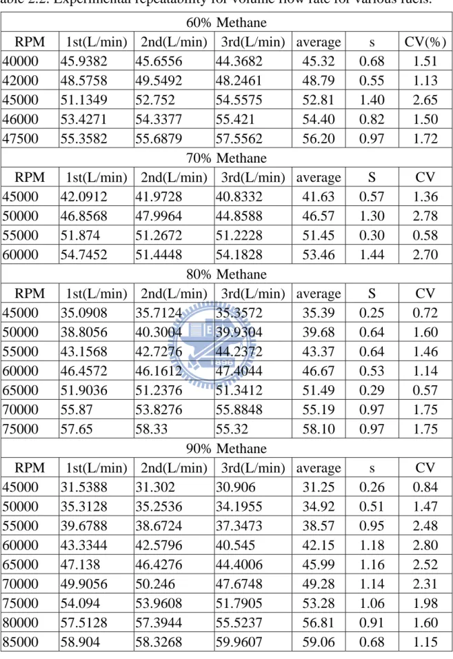
2.6.3 The Experimental Repeatability
To verify experimental accuracy, perform one test using the specified mixed fuel at the specified pressure and flow rate; perform each test three times to ensure experimental repeatability. The following examples demonstrate experimental repeatability. The volume flow rates for four fuels with LHVs and
28
RPMs are chosen to demonstrate experimental repeatability. The evaluation included three measurements for volume flow rate; the average value for each test was used. Standard deviation is defined as the absolute difference among the three volume flow rates. Table 2.2 and Fig. 2.7 show the coefficients of variation (CV) and experimental error bars. The CV is defined as the ratio of standard deviation s to mean X, where
s
is derived by∑
==
N 1 i 2 i-
X
)
(X
N
1
s
(2.3) The CV is a dimensionless number that can be used to specify the variation of data points in a data series around the mean. As the experiments were conducted outdoors, environmental conditions were difficult to control, for safety reason. As a consequence, the errors (<3%) in these experiments were expected to be higher than general experiment errors, but they should be acceptable. Experimental repeatability was apparently very high (Table 2.2).29
Table 2.2: Experimental repeatability for volume flow rate for various fuels. 60% Methane
RPM 1st(L/min) 2nd(L/min) 3rd(L/min) average s CV(%) 40000 45.9382 45.6556 44.3682 45.32 0.68 1.51 42000 48.5758 49.5492 48.2461 48.79 0.55 1.13 45000 51.1349 52.752 54.5575 52.81 1.40 2.65 46000 53.4271 54.3377 55.421 54.40 0.82 1.50 47500 55.3582 55.6879 57.5562 56.20 0.97 1.72 70% Methane
RPM 1st(L/min) 2nd(L/min) 3rd(L/min) average S CV 45000 42.0912 41.9728 40.8332 41.63 0.57 1.36 50000 46.8568 47.9964 44.8588 46.57 1.30 2.78 55000 51.874 51.2672 51.2228 51.45 0.30 0.58 60000 54.7452 51.4448 54.1828 53.46 1.44 2.70
80% Methane
RPM 1st(L/min) 2nd(L/min) 3rd(L/min) average S CV 45000 35.0908 35.7124 35.3572 35.39 0.25 0.72 50000 38.8056 40.3004 39.9304 39.68 0.64 1.60 55000 43.1568 42.7276 44.2372 43.37 0.64 1.46 60000 46.4572 46.1612 47.4044 46.67 0.53 1.14 65000 51.9036 51.2376 51.3412 51.49 0.29 0.57 70000 55.87 53.8276 55.8848 55.19 0.97 1.75 75000 57.65 58.33 55.32 58.10 0.97 1.75 90% Methane
RPM 1st(L/min) 2nd(L/min) 3rd(L/min) average s CV
45000 31.5388 31.302 30.906 31.25 0.26 0.84 50000 35.3128 35.2536 34.1955 34.92 0.51 1.47 55000 39.6788 38.6724 37.3473 38.57 0.95 2.48 60000 43.3344 42.5796 40.545 42.15 1.18 2.80 65000 47.138 46.4276 44.4006 45.99 1.16 2.52 70000 49.9056 50.246 47.6748 49.28 1.14 2.31 75000 54.094 53.9608 51.7905 53.28 1.06 1.98 80000 57.5128 57.3944 55.5237 56.81 0.91 1.60 85000 58.904 58.3268 59.9607 59.06 0.68 1.15
30
Chapter 3
Numerical analyses
3.1 Domain descriptions
The domain of combustion chamber consists of three major components. They are the solid annulus dual liners (inner and outer), which have several discharge holes, the vaporizing tube, which plays the role of fuel transportation, and the fluids, such as gas fuel and air, filling with the remaining spaces. The annulus combustor has twelve fuel tubes and the liner holes and relative components are in a periodic arrangement shown as Fig 3.1(a) and (b). Therefore, the combustor can be divided into one-twenty fourth sub-chambers geometrically as shown in Fig 3.1(c) and (d), which also represent the configuration of the full-size, three dimensional model domain employed for simulation. The components configuration of sub-chambers is shown as Fig. 3.2, and the size specification of sub-chamber is shown as Fig. 3.3.
3.2 Governing equations
In order to make the physical problem more tractable, several assumptions are made as follows:
1. One-twenty fourth annular zone of actual physical domain is considered due to symmetry, as shown in Fig. 3.1(c).
2. All gaseous mixtures are regarded as the ideal gases. 3. The flow is steady, compressible, and turbulent. 4. Properties in solid are constant.
31
6. One step global reaction is adopted to represent the chemical reaction of methane gas combustion.
7. Soret (or thermo) diffusion, accounting for the mass diffusion resulting from temperature gradients, is neglected [41].
Based on the assumptions mentioned above, the governing equations are given as follows [42]:
Mass conservation:
( )
=0 •∇ ρVv (3.1)
which describes the net mass flow across the control volume’s boundaries is zero.
Momentum conservation:
Based on the general Newton’s second law and particular viscous stress law, the momentum equations are developed as Navier-Stokes equations:
(
)
i ij i j j x p u u x ∂ ∂ − = − ∂ ∂ ρ τ (3.2) where suffixes i, and j represent Cartesian coordinates (i = 1,2,3), ui and uj are absolute fluid velocity components in directions of xi and xj , ρ is density, τij is shear stress tensor component, and p is pressure.In Newtonian fluid, the viscous stresses are proportional to the deformation rates of the fluid element. The nine viscous stress components can be related to velocity gradients to produce the following shear stress terms:
' ' 3 2 2 ij i j k k ij ij uu x u s μ δ ρ μ τ − ∂ ∂ − = (3.3)
32 ⎟ ⎟ ⎠ ⎞ ⎜ ⎜ ⎝ ⎛ ∂ ∂ + ∂ ∂ = i j j i ij x u x u s 2 1 , (3.4)
where μ is the molecular dynamic fluid viscosity, δij the ‘kronecker delta’, which is unity when i = j and zero otherwise, sij the rate of strain tensor.
For turbulent flow, ui, p and other dependent variables, including τij , assume their ensemble averaged values. Get back to Eq. 3.3, the rightmost term represents the additional Reynolds stresses due to turbulent motion. These are linked to the mean velocity field via the turbulence models. '
u is fluctuation about the ensemble average velocity and the overbar denotes the ensemble averaging process.
Energy conservation:
Heat transfer processes are computed by energy equation in the form known as the total enthalpy equation:
(
)
(
)
( )
i ij h j eff i u S x T k h u + ∂ ∂ + ∇ • ∇ = • ∇ ρ τ (3.5) where Sh are the energy sources, h is the total enthalpy and defined as:(
2 2 2)
2 1 w v u p i h= + + + + ρ (3.6)where iis internal energy. keff is the effective thermal conductivity of the material. In laminar flow, this will be the thermal conductivity of the fluid, k; In turbulent flow, t p t eff C k k Pr μ + = (3.7)
33
where Prt is the turbulent Prandtl number.
Species conservation:
(
)
i i j i i j i j j M x Y D x Y u x ρ ρ ⎟+ ω ⎟ ⎠ ⎞ ⎜ ⎜ ⎝ ⎛ ∂ ∂ ∂ ∂ = ∂ ∂ (3.8)where Yi represents mass fraction for mixture gas of CH4, O2, CO2, H2O and inert N2. The term Miωi is mass production rate of species. Mi is the molecular weight of i-th species. ω is global one-step reaction rate and in the Arrhenius form for methane combustion is computed as [43]:
2 4 O CH rY Y k = ω (3.9) where k is the reaction rate constant for methane combustion reaction:
Here four-step global reaction mechanism is adopted, the pre-exponential factor, temperature exponent and activation temperature are described as follows:
(1)Four-step global reaction mechanism 2 2 4 2H H 0 CO 4H CH + + → + (3.10) 2 2 2O CO H H CO+ → + (3.11) T T H M M H + → 2 + 2 (3.12) O H H O H2 2 2 2 2 3 + → + (3.13)
with the reaction rate expression as [43]: