A robust evolutionary algorithm for training neural networks

Ownership and Copyright

 Springer-Verlag London Limited 2001

A Robust Evolutionary Algorithm for Training Neural

Networks

Jinn-Moon Yang

_{and Cheng-Yan Kao}

1_{Department of Biological Science and Technology, National Chiao Tung University, Hsinchu, Taiwan} 2_{Department of Computer Science and Information Engineering, National Taiwan University, Taipei, Taiwan}

A new evolutionary algorithm is introduced for training both feedforward and recurrent neural net-works. The proposed approach, called the Family Competition Evolutionary Algorithm (FCEA), auto-matically achieves the balance of the solution quality and convergence speed by integrating multiple mutations, family competition and adaptive rules. We experimentally analyse the proposed approach by showing that its components can cooperate with one another, and possess good local and global properties. Following the description of implemen-tation details, our approach is then applied to sev-eral benchmark problems, including an artificial ant problem, parity problems and a two-spiral problem. Experimental results indicate that the new approach is able to stably solve these problems, and is very competitive with the comparative evolutionary algor-ithms.

Keywords: Adaptive mutations; Evolutionary

algor-ithm; Family competition; Multiple mutations; Neu-ral networks

1. Introduction

Artificial Neural Networks (ANNs) have been applied widely in many application domains. In addition to approximation capabilities for multilayer networks in numerous functions [1], ANNs avoid the bias of a designer in shaping system develop-ment owing to their flexibility, robustness and

toler-Correspondence and offprint requests to: J.-M. Yang, Department

of Biological Science and Technology, National Chiao Tung University, Hsinchu, Taiwan. E-mail: moon얀csie.ntu.edu.tw

ance of noise. Learning the weights of ANNs with fixed architectures can be formulated as a weight training process. This process is to minimise an objective function in order to achieve an optimal set of connection weights of an ANN which can be employed to solve the desired problems.

The standard back propagation learning algorithm [2] and many improved back propagation learning algorithms [3,4] are the widely used approaches. They are the gradient descent techniques which often try to minimise the objective function based on the total error between the actual output and the target output of an ANN. This error is used to guide the search of a back propagation approach in the weight space. However, the drawbacks with a back propa-gation algorithm do exist due to its gradient descent nature. It may get trapped in a local optima of the objective function, and is inefficient in searching for a global minimum of an objective function which is vast, multimodal and non-differentiable [5]. In addition, the back propagation approach needs to predetermine the learning parameters. Particularly, these applications where gradient methods are not directly applicable. Furthermore, from a theoretical perspective, gradient methods often produce worse recurrent networks than non-gradient methods when an application requires memory retention [6].

An evolutionary algorithm is a non-gradient method, and is a very promising approach for train-ing ANNs. It is considered to be able to reduce the ill effect of the back propagation algorithm, because it does not require gradient and differentiable infor-mation. Evolutionary algorithms have been success-fully applied to train or evolve ANNs in many application domains [5].

genetic algorithms [7], evolutionary programming [8] and evolution strategies [9]. Applying genetic algorithms to train neural networks may be unsatis-factory because recombination operators incur sev-eral problems, such as competing conventions [5] and the epistasis effect [10]. For better performance, real-coded genetic algorithms [11,12] have been introduced. However, they generally employ ran-dom-based mutations, and hence still require lengthy local searches near a local optima. In contrast,

evol-ution strategies and evolutionary programming

mainly use real-valued representation, and focus on self-adaptive Gaussian mutations. This type of mutation has succeeded in continuous optimisation, and has been widely regarded as a good operator for local searches [8,9]. Unfortunately, experiments [13] show that self-adaptive Gaussian mutation leaves individuals trapped near local optima for rugged functions.

Because none of these three types of original evolutionary algorithms is very efficient, many modifications have been proposed to improve the solution quality, and to speed up convergence. In particular, a popular method [14,15] is to incorporate local search techniques, such as the back propagation approach, into evolutionary algorithms. Such a hybrid approach possesses both the global optimality of the genetic algorithms, and also the convergence of the local searches. In other words, a hybrid approach can usually make a better trade-off between computational cost and the global opti-mality of the solution. However, for existing hybrid methods, local search techniques and genetic oper-ators often work separately during the search pro-cess.

Another technique is to use multiple genetic oper-ators [16,17]. This approach works by assigning a list of parameters to determine the probability of using each operator. Then, an adaptive mechanism is applied to change these probabilities to reflect the performance of the operators. The main disadvantage of this method is that the mechanism for adapting the probabilities may mislead evolutionary algor-ithms toward local optima.

To further improve the above approaches, in this paper a new method, called the Family Competition Evolutionary Algorithm (FCEA), is proposed for training the weights of neural networks. FCEA is a

multi-operator approach which combines three

mutation operators: decreasing-based Gaussian

mutation; adaptive Gaussian mutation; and self-adaptive Cauchy mutation. The performance of these three mutations heavily depends upon the same fac-tor, called step size. FCEA incorporates family com-petition [18] and adaptive rules for controlling step

sizes to construct the relationship among these three

mutation operators. Family competition is derived

from (1 ⫹ ␭)-ES [9], and acts as a local search

procedure. Self-adaptive mutation adapts its step sizes with a stochastic mechanism based on

perform-ance. In contrast, decreasing-based mutation

decreases the step sizes by applying a fixed rate ␥

where ␥ ⬍ 1.

FCEA markedly differs from previous approaches, because these mutation operators are sequentially applied with an equal probability of 1. In addition, each operator is designed to compensate for the disadvantages of the others, to balance the search power of exploration and exploitation. To the best of our knowledge, FCEA is the first successful attempt to integrate self-adaptive mutations and decreasing-based mutations by using family compe-tition and adaptive rules. Our previous work [19] has demonstrated that FCEA is competitive with the back propagation approach, and is more robust than several well-known evolutionary algorithms for reg-ular language recognition. In this paper, we modify the mutations to train both feedforward and recurrent networks for three complex benchmark problems. Experimental results show that FCEA is able to robustly solve these complex problems.

This paper is organised as follows. Section 2 describes the model of artificial neural networks trained by our FCEA. Section 3 describes FCEA in detail, and gives motivations and ideas behind vari-ous design choices. Next, Section 4 investigates the main characteristics of FCEA. We demonstrate experimentally how FCEA balances the trade-off between exploitation and exploration of the search. In Section 5, FCEA is applied to train a recurrent network for an artificial ant problem. Sections 6 and

7 present the experimental results of FCEA

employed to train feedforward networks for a two-spiral problem and N parity problems, where N ranges from 7 to 10. Conclusions are finally made in Section 8.

2. Artificial Neural Networks

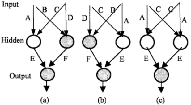
Figure 1 shows three general three-layer neural architectures that are able to arbitrarily approximate functions [1]. Figures 1(a) and (b) depict a fully connected feedforward network and a fully connec-ted feedforward network with shortcuts, respectively. Figure 1(c) shows a fully connected recurrent neural network with shortcuts. This network can be used to save contextual information via internal states, so that it becomes appropriate for tasks which must store and update contextual information. A shortcut

Fig. 1. Three kinds of general three-layer neural networks. (a) A fully connected feedforward network; (b) a fully connected feedforward network with shortcuts; and (c) a fully connected recurrent network with shortcuts.

is a connection link, which is directly connected from an input node to an output node. In this paper, our approach is applied to train the feedforward network shown in Fig. 1(a) for parity problems, the network shown in Fig. 1(b) with three hidden layers for a two-spiral problem, and the recurrent network shown in Fig. 1(c) for an artificial ant problem.

In FCEA, the formulation of training these archi-tectures in Fig. 1 is similar. Thus, only the architec-ture shown in Fig. 1(a) is considered when for-mulating the problem of training the weights of an ANN. Z, z1, %, zl, and Y, y1, %, ym, are the inputs

with l elements and the outputs with m nodes, respectively. The output values of the nodes in the hidden layer and in the output layer can be formulated as hj⫽ f

冉

冘

冊

冉

冘

冊

respectively, where f is the following sigmoid func-tion:

f(␩) ⫽ (1 ⫹ e⫺␩)⫺1 (3)

wijdenotes the weights between the input nodes and

hidden nodes, wjk denotes the weights between the

hidden nodes and output nodes, and q is the number of hidden nodes.

Our approach is to learn the weights of ANNs based on evolutionary algorithms. In FCEA, we optimise the weights (e.g. wij and wjk in Fig. 1(a))

to minimise the mean square error over a validation set containing T patterns:

Fig. 2. The competing conventions problem. The parents, (a) and (b), perform the same function and exhibit the same fitness value. Recombination creates an offspring (c) with two hidden neurons that perform nearly the same function.

F⫽ 1 Tm

冘

冘

where m is the number of output nodes, and Yk(It)

and Ok(It) are the actual and desired outputs of the output node k for the input pattern It. The

formu-lation is used as the fitness function of each individ-ual (an ANN) in FCEA, except for the artificial ant problem.

Applying recombination operators to train neural networks creates a particular problem called compet-ing conventions [5]. Under these circumstances, the objective function may become a many-to-one func-tion, because different networks may perform the same function and exhibit the same fitness value, as illustrated by two examples shown in Figs 2(a) and (b). Given two such networks, recombination creates an offspring with two hidden neurons that perform nearly the same function. The performance of the offspring (Fig. 2(c)) is worse than its parents (i.e. the networks shown in Figs 2(a) and (b)), because it is unable to perform the function of the other hidden neuron. The number of competing conventions grows exponentially with the number of hidden neurons [5].

3. Family Competition Evolutionary

Algorithm

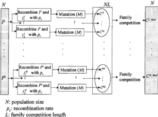
In this section, we present details of the Family Competition Evolutionary Algorithm (FCEA) for training both feedforward and recurrent neural net-works. The basic structure of the FCEA is as follows (Fig. 3): N individuals (ANNs) are generated as the initial population. Then FCEA enters the main evolutionary loop, consisting of three stages in every iteration: decreasing-based Gaussian mutation; self-adaptive Cauchy mutation; and self-self-adaptive Gaus-sian mutation. Each stage is realised by generating

Fig. 3. Overview of our algorithm: (a) FCEA (b) FCFadaptive procedure.

a new quasi-population (with N ANNs) as the parent of the next stage. As shown in Fig. 3, these stages differ only in the mutations used and in some parameters. Hence, we use a general procedure, ‘FCFadaptive’, to represent the work done by these stages.

The FCFadaptive procedure employs three para-meters (the parent population (P, with N solutions), mutation operator (M) and family competition length (L)) to generate a new quasi-population. The main work of FCFadaptive is to produce offspring, and then conduct the family competition (Fig. 4). Each individual in the population sequentially becomes the ‘family father’. Here we use I1 _{as the ‘family} father’ to describe the procedure of family compe-tition. With a probability pc, this family father and

another ANN (I1

m1) randomly chosen from the rest

of the parent population are used as parents to do a recombination operation. Then the new offspring or the family father (if the recombination is not

Fig. 4. The main steps of the family competition.

conducted) is operated on by the mutation to gener-ate an offspring (C11_{). For each family father, such} a procedure is repeated L times. Finally, L ANNs (C11_{, %, C}1L_{) are produced, but only the one (C}1Fbest₎ with the lowest objective value survives. Since we create L ANNs from one ‘family father’ and perform a selection, this is a family competition strategy. We think this is a way not only to avoid the premature, but also to keep the spirit of local search-es.

After the family competition, there are N parents and N children left. Based on different stages, we employ various ways of obtaining a new quasi-population with N individuals (ANNs). For both Gaussian and Cauchy self-adaptive mutations, in each of the pairs of father and child, the individual with a better objective value survives. This is the so-called ‘family selection’. On the other hand, ‘population selection’ chooses the best N individuals from all N parents and N children. With a probability

Pps, FCEA applies population selection to speed up

the convergence when the decreasing-based Gaus-sian mutation is used. For the probability (1-Pps),

family selection is still considered. To reduce the ill effects of greediness on this selection, the initial

Ppsis set to 0.05, but it is changed to 0.5 when the

mean step size of self-adaptive Gaussian mutation is larger than that of decreasing-based Gaussian mutation. Note that the population selection is simi-lar to (␮⫹␮)-ES in the traditional evolution stra-tegies. Hence, through the process of selection, the FCFadaptive procedure forces each solution of the starting population to have one final offspring. Note that we create LN offspring in the FCFadaptive procedure but the size of the new quasi-population remains the same as N.

For all three mutation operators, we assign differ-ent parameters to control performance. Such para-meters must be adjusted through the evolutionary process. We modify them first when mutations are applied. Then, after the family competition is com-plete, parameters are adapted again to better reflect the performance of the whole FCFadaptive pro-cedure.

In the rest of this section, we explain the chromo-some representation and each important component of the FCFadaptive procedure: recombination oper-ators, mutation operations, and rules for adapting step sizes (␴, v and ␺).

3.1. Chromosome Representation and Initialisation

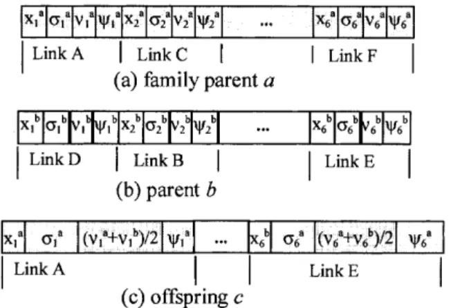
Regarding chromosome representation, we present each solution of a population as a set of four

n-Fig. 5. Chromosome representation and recombination operators. (a) and (b) represent the networks shown in Figs 2(a) and (b), respectively; (c) is an offspring generated from (a) and (b) in the self-adaptive Gaussian mutation stage.

dimensional vectors (x, ␴, v, ␺), where n is the number of weights of an ANN. The vector x is the weights to be optimised;␴, v and ␺ are the step-sise vectors of decreasing-based mutations, self-adaptive

Gaussian mutation, and self-adaptive Cauchy

mutation, respectively. In other words, each solution

x is associated with some parameters for step-sise

control. Figure 5 depicts three chromosome rep-resentations which represent the respective networks shown in Fig. 2. In these cases, n is 6. Here, the initial value of each entry of x is randomly chosen over [⫺0.1, 0.1], and the initial values of each entries of the vectors ␴, v and ␺ are set to be 0.4, 0.1 and 0.1, respectively. For easy description of the operators, we use a ⫽ (xa_, ␴a_{, v}a_, ␺a_{) to}

represent the ‘family father’ and b ⫽ (xb_, ␴b_{, v}b_,

␺b_{) as another parent (for the recombination operator}

only). The offspring of each operation is represented as c ⫽ (xc_, ␴c_{, v}c_, ␺c_{). We also use the symbol x}d j

to denote the jth component of an individual d, ∀j 苸 {1, %, n}.

3.2. Recombination Operators

FCEA implements two recombination operators to generate offspring: modified discrete recombination; and intermediate recombination [9]. With prob-abilities 0.9 and 0.1, at each stage only one of the two operators is chosen. Probabilities are set to obtain good performance according to our experi-mental experience. Here we again mention that recombination operators are activated with only a probability pc. The optimising connection weights

(x) and a step size (␴, v or ␺) are recombined in a recombination operator.

Modified discrete recombination: the original

dis-crete recombination [9] generates a child that inherits genes from two parents with equal prob-ability. Here the two parents of the recombination operator are the ‘family father’ and another solution randomly selected. Our experience indicates that FCEA can be more robust if the child inherits genes from the ‘family father’ with a higher probability. Therefore, we modified the operator to be as fol-lows: xc j ⫽

再

Intermediate recombination: we define intermediate

recombination as:

xc

j ⫽ xaj ⫹ 0.5 (xbj ⫺ xaj) and (6)

wc

j ⫽ waj ⫹ 0.5 (wbj ⫺ waj) (7)

where w is v, ␴, or ␺ based on the mutation operator applied in the family competition. For example, if self-adaptive Gaussian mutation is used in this FCFadaptive procedure, x in Eqs (6) and (7) is v. We follow the work of the evolution strategies community [20] to employ only intermediate recom-bination on step-size vectors, that is, ␴, v and ␺. To be more precise, x is also recombined when the intermediate recombination is chosen.

Figure 5 shows a recombination example in the self-adaptive Gaussian mutation stage. The offspring (c) is generated from the ‘family father’ (a) and another parent (b) by applying the modified discrete recombination for the connection weights x and the intermediate recombination for the step size v. In other words, the ␴ and ␺ are unchanged in the self-adaptive Gaussian mutation stage.

3.3. Mutation Operators

Mutations are the main operators of the FCEA. After recombination, a mutation operator is applied to the ‘family father’ or the new offspring generated by a recombination. In FCEA, the mutation is per-formed independently on each vector element of the selected individual by adding a random value with expectation zero:

x⬘i⫽ xi⫹ wD(·) (8)

ith variable of x⬘ mutated from x, D(·) is a random

variable, and w is the step size. In this paper, D(·) is evaluated as N(0, 1) or C(1) if the mutations are, respectively, Gaussian mutation or Cauchy mutation.

Self-adaptive Gaussian mutation: we adapted Schwefel’s [21] proposal to use self-adaptive Gaus-sian mutation in training ANNs. The mutation is accomplished by first mutating the step size vj and

then the connection weight xj:

vc

j ⫽ vaj exp[␶⬘N(0, 1)⫹␶Nj(0, 1)] (9)

xc

j ⫽ xaj ⫹ vcjNj(0, 1) (10)

where N(0, 1) is the standard normal distribution.

Nj(0, 1) is a new value with distribution N(0, 1)

that must be regenerated for each index j. For FCEA, we follow Ba¨ck and Schwefel [20] in setting ␶ and ␶⬘ as (

冑

冑

Self-adaptive Cauchy mutation: a random variable

is said to have the Cauchy distribution (苲C(1)) if it has the following density function:

f(x; t)⫽ t/␲

t2⫹ x2, ⫺ ⬁ ⬍ x ⬍ ⬁ (11)

We define self-adaptive Cauchy mutation as follows: ␺c

j ⫽␺aj exp[␶⬘N(0, 1)⫹␶Nj(0, 1)] (12)

xc

j ⫽ xaj ⫹␺cj(t) (13)

In our experiments, t is 1. Note that self-adaptive Cauchy mutation is similar to self-adaptive Gaussian mutation, except that Eq. (10) is replaced by Eq. (13). That is, they implement the same step-sise control, but use different means of updating x.

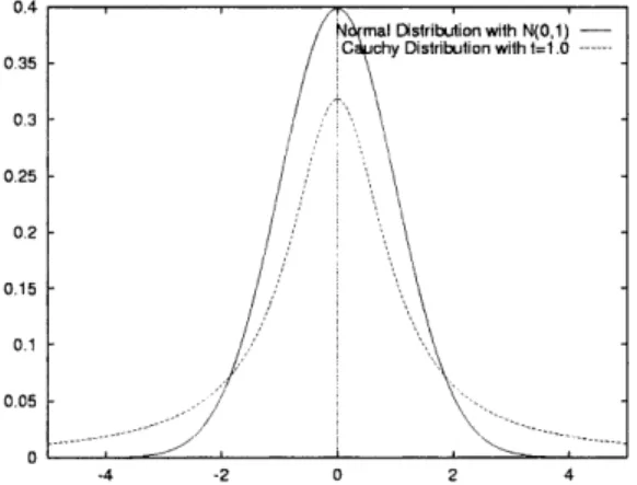
Figure 6 compares the density functions of Gaus-sian distribution (N(0, 1)) and Cauchy distributions (C(1)). Clearly, Cauchy mutation is able to make a larger perturbation than Gaussian mutation. This implies that Cauchy mutation has a higher

prob-Fig. 6. Density function of Gaussian and Cauchy distributions.

ability of escaping from local optima than does Gaussian mutation. However, the order of local convergence is identical for Gaussian and spherical Cauchy distributions, while non-spherical Cauchy mutations lead to slower local convergence [22].

Decreasing-based Gaussian mutations: our

decreas-ing-based Gaussian mutation uses the step-sise vec-tor ␴ with a fixed decreasing rate ␥ ⫽ 0.97 as fol-lows:

␴c⫽␥␴a ₍₁₄₎

xc

j ⫽ xaj ⫹␴cNj(0, 1) (15)

Previous results [13] have demonstrated that self-adaptive mutations converge faster than decreasing-based mutations, but for rugged functions, self-adaptive mutations are more easily trapped into local optima than decreasing-based mutations.

It can be seen that step sizes are the same for

all components of xa _{in the decreasing-based}

mutation, but are different in the self-adaptive mutations. This means two types of mutations have different search behaviour. For decreasing-based mutation, it is like we search for a better child in a hypersphere centred at the parent. However, for self-adaptive mutation, the search space becomes a hyperellipse. Figure 7 illustrates this difference using two-dimensional contour plots.

Fig. 7. (a) and (b) show the difference of search space between self-adaptive and decreasing-based mutations. Using two-dimen-sional contour plots, the search space from parents are ellipses and circles.

3.4. Adaptive Rules

The performance of Gaussian and Cauchy mutations is largely influenced by the step sizes. FCEA adjusts the step sizes while mutations are applied (e.g. Eqs (9), (12) and (14)). However, such updates insufficiently consider the performance of the whole

family. Therefore, after the family competition, some additional rules are implemented:

1. A-decrease-rule: immediately after self-adaptive mutations, if the objective values of all offspring are greater than or equal to that of the ‘family father’, we decrease the step-sise vectors v (Gaussian) or ␺ (Cauchy) of the parent:

wa

j ⫽ 0.97waj (16)

where wa _{is the step size vector of the parent.}

In other words, if there is no improvement after self-adaptive mutations, we may propose a more conservative implementation. That is, a smaller step size tends to result in a better improvement in the next iteration. This follows the 1/5-success rule of (1⫹␭)-ES [9].

2. D-increase-rule: it is difficult, however, to decide the rate ␥ of decreasing-based mutations. Unlike self-adaptive mutations, which adjust step sizes automatically, its step size goes to zero as the number of iterations increases. Therefore, it is essential to employ a rule which can enlarge the step size in some situations. The step size of the decreasing-based mutation should not be too small when compared to the step sizes of self-adaptive mutations. Here, we propose to increase ␴ if either of the two self-adaptive mutations generates better offspring. To be more precise, after a self-adaptive mutation, if the best child with a step size v is better than its ‘family father’, the step size of the decreasing-based mutation is updated as follows:

␴c

j ⫽ max (␺cj,␤vcmean) (17)

where vc

mean is the mean value of the vector v,

and ␤ is 0.2 in our experiments. Note that this

rule is applied in stages of self-adaptive

mutations, but not of decreasing-based mutations. From the above discussions, the main procedure of FCEA is implemented as follows:

1. Set the initial step sizes (␴, v and ␺), family competition lengths (Ld and La), and crossover

rate (pc). Let g ⫽ 1.

2. Randomly generate an initial population, P(g), with N networks. Each network is represented as (xi_, ␴i_{, v}i_, ␺i_), ∀i 苸 {1, 2, %, N}.

3. Evaluate the fitness of each network in the popu-lation P(g).

4. repeat

4.1 {Decreasing-based Gaussian mutation (Mdg)}

• Generate a children set, CT, with N networks

by calling FCFAdaptive with parameters:

P(g), Mdg and Ld. That is, P1(g) ⫽

FCFAdaptive(P(g), Mdg, Ld).

• Select the best N networks as a new quasi-population, P1(g), by population selection from the union set {P(g) 傼 CT with

prob-ability Pps or by family selection with 1

⫺ Pps.

4.2 {Self-adaptive Cauchy mutation (Mc)}:

Gen-erate a new children set, CT, by calling

FCFAdaptive with parameters: P1(g), Mc and

La. Apply family selection to select a new

quasi-population, P2(g), with N networks from the union set {P1(g) 傼 CT.

4.3 {Self-adaptive Gaussian mutation (Mg)}:

Generate a new children set, CT, by calling

FCFAdaptive with parameters: P2(g), Mg and

La. Apply family selection to select a new

quasi-population, Pnext, with N networks from

the union set P2(g) 傼 CT.

4.4 Let g ⫽ g ⫹ 1 and P(g) ⫽ Pnext.

until (termination criterion is met).

Output the best solution and the objective function value.

On the other hand, the FCFadaptive proceeds along the following steps:

{Parameters: P is the working population, M is the applied mutation (Mdg, Mg or Mc), and L denotes

the family competition length (La or Ld).}

1. Let C be an empty set (C ⫽ ␪).

2. for each network a, called family father, in the population with N networks

2.1 for l ⫽ 1 to L {Family Competition} • Generate an offspring c by using a

recombi-nation (c ⫽ recombination (a,b)) with prob-ability pc or by copying the family father a

to c (c ⫽ a) with probability 1 ⫺ pc.

• Generate an offspring cl by mutating c as

follows:

cl⫽

冦

Mdg(c) if M is Mdg; {decreasing-based Gaussian mutation}

Mg(c) if M is Mg; {self-adaptive Gaussian mutation}

Mc(c) if M is Mc; {self-adaptive Cauchy mutation}

endfor

2.2 Select the one (cbest_{) with the lowest objective}

value from c1, %, cL. {family selection}

2.3 Apply adaptive rules if M is a self-adaptive mutation operator (Mc or Mg)

• Apply A-decrease-rule to decrease the step sizes (␺ or v) of Mc or Mg if the objective

value of the family father a is lower than cbest_.

That is, wa

j ⫽ 0.97waj.

• Apply D-increase-rule to increase the step size (␴) of Mdg if the objective value of the family

father a is larger than cbest_{. That is,} ␴best j ⫽ max(␴best j ,␤v best mean).

2.4 Add the cbest _{into the set C.}

endfor

Return the set C with N networks.

4. A Study of some Characteristics of

FCEA

In this section, we discuss several characteristics of FCEA by numerical experiments and mathematical explanations. First, we experimentally discuss the effectiveness of using the family competition and multiple mutations. Next, we explore the importance of controlling step sizes and of employing adaptive rules, i.e. A-decrease and D-increase rules.

To analyse FCEA, we study a 2-bit adder [23] and a parity problem by using feedforward networks, which are similar to Fig. 1(a). A 4–4–3 network is employed to solve the 2-bit adder problem. The fully connected ANN has 35 connection weights and 16 input patterns. The output pattern is the result of the sum of the two 2-bits input strings. In addition, a 4–4-1 network is used for solving the parity problem. The fully connected ANN has 25 connection weights and 16 input patterns. The output value is 1 if there is an odd number of 1s in the input patterns.

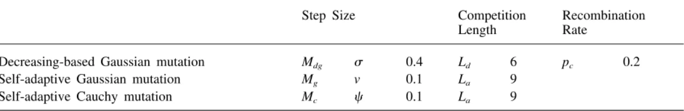
Evolution begins by initialising all the connection weights x of each network to random values between -0.1 and 0.1. The initial values of step sizes for decreasing-based Gaussian mutations, self-adaptive Gaussian mutation and self-self-adaptive Cau-chy mutation are set to 0.4, 0.1 and 0.1, respectively. Table 1 indicates the settings of FCEA parameters, such as the family competition length and the cross-over rate (pc). Ld and ␴ are the parameters for the

decreasing-based mutation; La, v and ␺ are for

self-adaptive mutations. The same parameter settings are used for all testing problems studied in this work.

In this paper, Sr denotes the percentage of an

approach classifying all training data correctly, and

FE denotes the number of average function

evalu-Table 1. Parameter settings and notations.

Step Size Competition Recombination Length Rate

Decreasing-based Gaussian mutation Mdg ␴ 0.4 Ld 6 pc 0.2

Self-adaptive Gaussian mutation Mg v 0.1 La 9

Self-adaptive Cauchy mutation Mc ␺ 0.1 La 9

ations of an approach satisfying the terminal con-ditions. That is, an approach correctly classifies all training data or exhausts the number of maximum function evaluations.

4.1. The Effectiveness of the Family Competition

Because the family competition length is the critical factor in FCEA, we investigate the influence of La

and Ld. FCEA is implemented on the parity and

2-bit adder problems on various family lengths, i.e.

La ⫽ Ld ⫽ L, where L ranges from 1 to 9. In other

words, the sums of the total length (i.e. Ld ⫹ 2La)

are from 3 to 27 in one generation. FCEA executes each problem over 50 runs on each length. The

number of maximum function evaluations is

700,000. The Sr and FE of FCEA are calculated

based on 50 independent runs. Figure 8(a) shows that the performance of FCEA is unstable when the total length is below 9 (Ld ⫹ 2La ⱕ 9), and FCEA

has the worst performance when both La and Ld are

set to 1. The performance of FCEA becomes stable while the total length exceeds 15.

Figures 8(b) and 8(a) show that the FE of FCEA is decreasing and the Sr is increasing when the

family competition length (L) is increased from 1 to 4. On the other hand, the FE of FCEA is increasing, but the Sr is stable while both La and

Ld exceed 8. From the above observations, we know

that the family competition length is important for our FCEA. Therefore, we set La to 9 and Ld to 6

for all testing problems studied in this paper.

4.2. The Effectiveness of Multiple Operators

Using multiple mutations in each iteration is one of the main features of FCEA. With family selection, FCEA uses a high selection pressure along with a diversity-preserving mechanism. With a high selec-tion pressure, it become necessary to use highly disruptive search operators, such as the series of three mutation operators used in FCEA. Using

Fig. 8. The percentages (Sr) of FCEA classifying all training data correctly and the numbers (FE) of average function evaluations of

FCEA on different family competition lengths. Each problem is tested over 50 runs for each length.

numerical experiments, we will demonstrate that the three operators cooperate with one another, and possess good local and global properties.

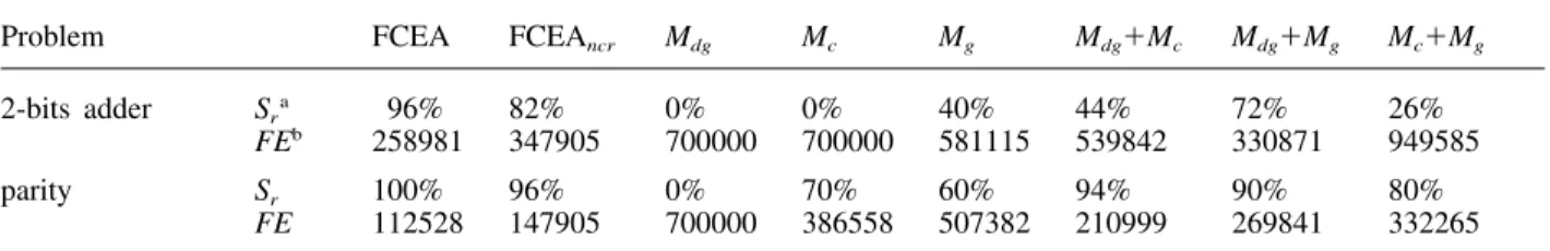
We compare eight different uses of mutation oper-ators in Table 2. Each use combines some of the three operators applied in FCEA: decreasing-based

Gaussian mutation (Mdg); self-adaptive Cauchy

mutation (Mc); and self-adaptive Gaussian mutation

(Mg). For example, the Mc approach uses only

self-adaptive Cauchy mutation; the Mdg ⫹ Mc approach

integrates decreasing-based Gaussian mutation and self-adaptive Cauchy mutation; and FCEA is an approach integrating Mdg, Mc and Mg. The FCEAncr

approach is a special case of FCEA without adaptive rules, i.e. without the A-decrease-rule (Eq. (16)) and D-increase-rule (Eq.(17)). Except for FCEAncr, the

others employ adaptive rules. To have a fair com-parison, we set the family competition length (L) of all eight approaches to the same value. For example,

if Ld ⫽ 6 and La ⫽ 9 in FCEA, L ⫽ 24 for

one-operator approaches (Mdg, Mc and Mg) and Ld ⫽ La

⫽ 12 for two-operator approaches (Mdg ⫹ Mc, Mdg

⫹ Mg and Mc ⫹ Mg).

There are some observations from experimental results:

1. Generally, strategies with a suitable combination

Table 2. Comparison of various approaches of FCEA on the 2-bit adder problem and the parity problem. Mdg, Mc and Mg represent different mutations used in FCEA.

Problem FCEA FCEAncr Mdg Mc Mg Mdg⫹Mc Mdg⫹Mg Mc⫹Mg

2-bits adder Sra 96% 82% 0% 0% 40% 44% 72% 26% FEb _{258981 347905 700000 700000 581115 539842 330871 949585}

parity Sr 100% 96% 0% 70% 60% 94% 90% 80%

FE 112528 147905 700000 386558 507382 210999 269841 332265

a_S

r denotes the percentage of an approach classifying all training data correctly.

b_{FE denotes the number of average function evaluations.}

of multiple mutations (FCEA and Mdg ⫹ Mg)

perform better than unary-operator strategies, in terms of the solution quality. However, the num-ber of function evaluations does not increase much when using multi-operator approaches. Sometimes, the number even decreases (e.g. FCEA verses Mdg). Overall, FCEA has the best

performance and the number of function evalu-ations is very competitive.

2. The adaptive rules applied to control step sizes are useful according to the comparison of

FCEAncr and FCEA. We made similar

obser-vations when FCEA was applied in global optimisation [13].

3. Each mutation operator (Mdg, Mc and Mg) has a

different performance. Table 2 shows that self-adaptive mutations (Mc and Mg) outperform the

decreasing-based mutation (Mdg) on training

neu-ral networks.

4. The approaches combining decreasing-based

mutation with self-adaptive mutation (Mdg ⫹ Mc

or Mdg ⫹ Mg) perform better than that combining

two self-adaptive mutations (Mc⫹Mg). These

results can be analysed as follows: Figure 7 indicates that the distribution of the one-step perturbation of Mdg is different from that of Mc

or Mg. The former approach (Mdg ⫹ Mc or Mdg

⫹ Mg) applies decreasing-based mutation with

large initial step sizes as a global search strategy and the self-adaptive mutations with the family competition procedure and replacement selection as local search strategies. Therefore, we suggest that a global optimisation method should consist of both global and local search strategies.

4.3. Controlling Step Sizes

Numerical experiments in the previous subsection have not fully shown the importance of controlling the step sizes. Here we would like to further discuss this issue by analysing the mean step sizes and the mean expected improvement in the whole iterative process. First, we denote AT(O) as the mean value of

the step size of an operator O at the Tth generation:

AT(O)⬅

冉

冘

冉

冘

冊

冊

where N is the population size, n represents the number of weights, and wki is the step size of the

ith component of the kth individual in the

popu-lation. Thus, w is ␴ for Mdg and is ␺ for Mc.

Secondly, we define ET(O), the expected

improve-ment of all offspring, by an operator O at the

Tth generation: ET(O)⬅

冉

冘

冉

冘

冊

冊

where L is the family competition length and ckl is

the lth child generated by the kth ‘family father’ ak.

Figures 9–14 show the curves of AT(O) and ET(O)

on the 2-bit adder problem because FCEA, FCEAncr,

Fig. 9. The average step sizes of various mutations in FCEA.

Fig. 10. The average expected improvements of various mutations in FCEA.

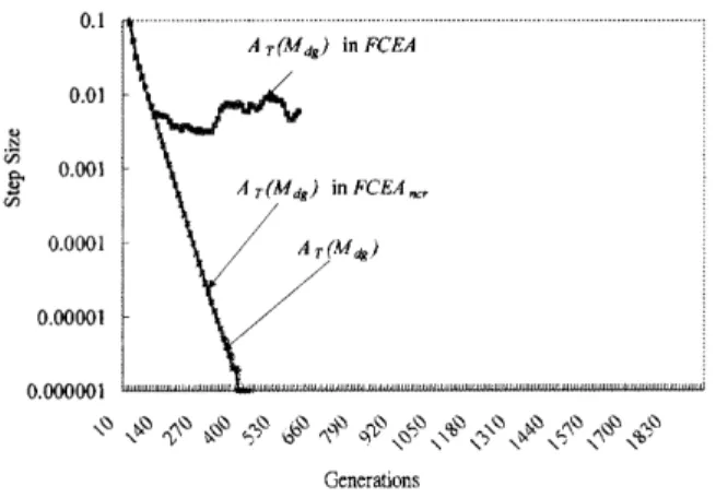
Fig. 11. The average step sizes of decreasing-based Gaussian of FCEA, FCEAncr and Mdg.

Fig. 12. The average step sizes of self-adaptive Gaussian mutation of FCEA, FCEAncr and Mg.

Mdg and Mg have a greatly different performance

on it. Figures 9 and 10 illustrate the behaviour of each mutation in FCEA, while Figs 11–14 present

AT(O) and ET(O) of Mdg and Mg in three different

evolutionary processes: Mdg or Mg itself, FCEA, and

Fig. 13. The average expected improvement of the decreasing-based Gaussian mutation of FCEA, FCEAncr and Mdg.

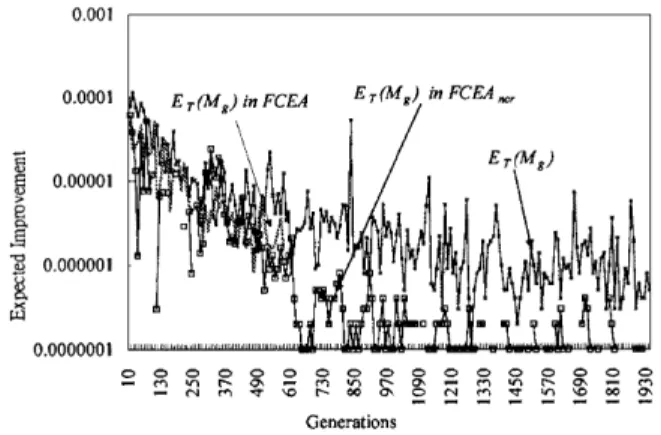
Fig. 14. The average expected improvement of self-adaptive Gaussian mutation of FCEA, FCEAncr and Mg.

because its behaviour is similar to Mg. Some

inter-esting observations are given below.

1. The control of step sizes is important because the performance of mutations used in FCEA heavily depend upon step sizes based on Figs 9–14. For example, Fig. 11 shows that the step sizes of decreasing-based Gaussian mutations in FCEAncr

and in Mdg approach zero while the number of

the generations exceeds 450. Figure 13 shows that their respective expected improvement also approaches zero.

2. Self-adaptive mechanisms and family competition are applied to adjust step sizes and to retain children with better function values. From Fig. 9, it can be seen that, in FCEA, the step size of

Mc is always smaller than that of Mg. Note that

Cj(1) in Eq. (13) tends to be larger than Nj(0, 1)

in Eq. (10). However, it seems that a small perturbation from the parent decreases the func-tion value more easily than a large one. For example, Fig. 12 indicates that AT(Mg) in

FCEAncr is larger than that in Mg. Figure 14

shows that the respective ET(Mg) in FCEAncr is

smaller than that in Mg. Hence, a self-adaptive

mechanism and the family competition cause children with smaller step sizes to survive after Cauchy mutation.

3. FCEA performs better than FCEAncr due to the

implementation of the D-increasing and

A-decreasing rules. Figure 11 shows that the

average step size, AT(Mdg) in FCEA, of the

decreasing-based mutation is controlled by the D-increasing rule after the 120th generation. In FCEAncr, the average step size is decreased with

a fixed rate and becomes very small because the D-increasing rule is not applied. Furthermore, Fig. 12 indicates that the average step size of

Mg in FCEAncr is larger than FCEA, because the

A-decreasing rule is not applied in FCEAncr.

Figure 14 shows that ET(Mg) in FCEAncr is

smaller than that in Mg. These observations may

explain the effectiveness of adaptive rules. 4. The mutation operators used in FCEA have a

similar average expected improvement, although their step sizes are different according to Figs 10 and 9. This implies that each mutation is able to improve solution quality by adapting its step sizes in the whole searching process.

In summary, the above discussion has shown that the main ideas of FCEA, employing multiple mutation operators in one iteration and coordinating them by adaptive rules, are very useful.

4.4. Comparison with Related Works

Finally, we compare FCEA with three GENITOR style genetic algorithms [23], including a bit-string genetic algorithm (GENITOR), a distributed genetic algorithm (GENITOR II) and a real-valued genetic algorithm. GENITOR, proposed by Whitley et al. [23] to train ANNs, is one of the most widely used genetic algorithms. GENITOR encoded weights as a binary string to solve 2-bit adder problem. This approach found solutions on 17 out of 30 runs, i.e.

Sr ⫽ 56%, by using a population of 5000 and two

million function evaluations. GENITOR II [23] used a combination of adaptive mutation and a distributed genetic algorithm. It was able to increase the Sr to

93% on a 2-bit adder problem. However, its popu-lation size was also 5000, and the number of func-tion evaluafunc-tions also reached two million. A back propagation method was implemented [23] to solve the 2-bit adder problem, and its convergence rate is 90%.

At the same time, Whitley et al. duplicated a real-valued genetic algorithm, proposed by Montana and Davis [16]. This algorithm is able to evolve both

Table 3. Comparison of FCEA with three GENITOR style genetic algorithms, including GENITOR, GENITOR II and

real-value representation GENITOR on the 2-bit adder problem.

Problem FCEA GENITORc _{GENITOR II Real-valued GENITOR}

2-bits adder Sa _{96% 56% 93% 90%}

FEb _{258,981 2,000,000 2,000,000 42,500}

a_S

r denotes the percentage of an approach classifying all training data correctly.

b_{FE denotes the number of average function evaluations.}

c_{All results of GENITOR style genetic algorithms are directly summarised from Whitley et al. [23].}

the architecture and the weights. In this experiment, the convergence (Sr) is 90% on a 2-bit adder

prob-lem using a population of 50. The number of aver-age function evaluations was 42,500.

In contrast to these approaches, FCEA needs 258,981 function evaluations, and the Sr is up to

96% using small population size, i.e. 30. These results are summarised in Table 3.

5. The Artificial Ant Problem

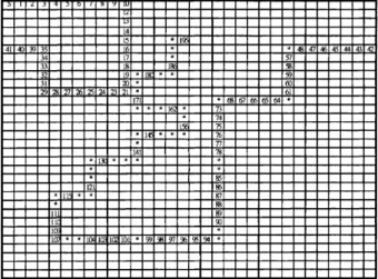
In this section, we study an artificial ant problem, i.e. tracker task ‘John Muir Trail’ [24]. In this problem, a simulated ant is placed on a two-dimen-sional toroidal grid that contains a trail of food. The ant traverses the grid to collect any food encountered along the trail. This task requires us to train a neural network (i.e. a simulated ant) that collects the maximum number of pieces of food during the given time steps. Figure 15 presents this trail. Each black box in the trail stands for a food unit. Accord-ing to the environment of Jefferson et al. [24], the ant stands on one cell, facing one of the cardinal directions; it can sense only the cell ahead of it. After sensing the cell ahead of it, the ant must take

Fig. 15. The ‘John Muir Trail’ artificial ant problem. The trail is a 32× 32 toroidal grid where the right edge is connected to left edge. The symbol 쮿 denotes a food piece on the trail, and → denotes the start position and starting facing direction of an ant.

one of four actions: move forward one step, turn right 90°, turn left 90°, and no-op (do nothing). In the optimal trail, there are 89 food cells, 38 no food cells and 20 turns. Therefore, the number of mini-mum steps for eating all food is 147 time steps.

To compare with previous research, we follow the work of Jefferson et al. [24]. That investigation used not only finite state machines and recurrent neural networks to represent the problem, but also a traditional bit-string genetic algorithm to train the architectures. The recurrent network used for controlling the simulated ant is the full connection with shortcuts architecture shown in Fig. 1(c). Each simulated ant is controlled by a network having two input nodes and four output nodes. The ‘food’ input is 1 when the food is present in the cell ahead of the ant; and the second ‘no-food’ is 1 in the absence of the food in the cell in front of the ant. Each output unit corresponds to a unique action: move forward one step, turn right 90°, turn left 90°, or no-op. Each input node is connected to each of the five hidden nodes and to each of the four output nodes. The five hidden nodes are fully connected in the hidden layer. Therefore, this architecture is a

Fig. 16. A travelled solution of the ‘John Muir Trail’ within 195 time steps of a simulated ant controlled by our evolved neural controller. The number in the cell is the order in which the ant eats the food. The symbol * in the entry represents a cell travelled by the ant.

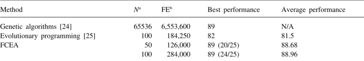
Table 4. Comparison among the genetic algorithm, evolutionary programming and our FCEA on the ‘John Muir Trail’

ant problem. The first number in parentheses is the number of runs finding all 89 food peices, and the second number is the number of total runs.

Method Na _FEb _{Best performance Average performance}

Genetic algorithms [24] 65536 6,553,600 89 N/A Evolutionary programming [25] 100 184,250 82 81.5

FCEA 50 126,000 89 (20/25) 88.68

100 284,000 89 (24/25) 88.96

a_{N is the population size. N/A denotes the result not available in the literature.} b_{FE denotes the average numbers of function evaluations.}

full connection with shortcuts recurrent neural net-work; its total number of links with bias input is 72. To compare with previous results, the fitness is defined as the number of pieces of food eaten within 200 time units.

Figure 16 depicts a typical search behaviour and the travelled path of a simulated ant that is con-trolled by our evolved neural network. The number in the cell is the time step to eat the food. The symbol * denotes a cell travelled by an ant when the cell is empty. Figure 16 indicates that the ant requires 195 time steps to seek all 89 food pieces in the environment.

Table 4 compares our FCEA, evolutionary pro-gramming [25], and genetic algorithm [26] on the artificial ant problem. Jefferson et al. [24] used tra-ditional genetic algorithms to solve the ‘John Muir Trail’. That investigation encoded the problem with 448 bits, and used a population of 65,536 to achieve the task in 100 generations. Their approach required 6,553,600 networks to forage 89 food pieces within exactly 200 time steps. In contrast to Jefferson et al.’s solution, our FCEA uses population sizes of 50 and 100, and only requires about 126,000 and 284,000 function evaluations, respectively, to eat 89 food pieces within 195 time steps. Table 4 also indicates that FCEA performs much better than evol-utionary programming [25], which uses a population of 100, and the average number of function evalu-ations is about 184,250. The best fitness value of evolutionary programming is 82, and its solution quality is worse than FCEA.

6. The Two-spiral Problem

In the neural network community, learning to tell two spirals apart is a benchmark task which is an extremely hard classification task [3,4,26,27]. The learning goal is to properly classify all the training

data (97 points on each spiral, as shown in Fig. 17(a)) which lie on two distinct spirals in the x-y plane. These spirals coil three times around the origin and around one another. The data of the two-spiral problem is electronically available from the Carnegie-Mellon University connectionist bench-mark collection. We follow the suggestion of Fahl-man and Lebiere [3] to use 40-20-40 criterion. That is, an output is considered to be a logical 0 if it lies in [0, 0.4], to be a logical 1 if the output lies in [0.6, 1.0], and indeterminate if it lies in [0.4, 0.6]. In the testing phase, 20,000 points are chosen

regularly from the space (i.e. ⫺10 ⱕ x ⱕ 10 and

⫺10 ⱕ y ⱕ 10), and the output of the system is defined as in the training phase.

Lang and Withbrock [26] used a 2-5-5-5-1 net-work with shortcut connections. Each node is con-nected to all nodes in all subsequent layers. With one additional bias connection for each node, there-fore, there is a total of 138 trainable weights in the network. They employed the standard back propa-gation approach to train this network, and considered the task to be completed when each of the 194 points in the training set responded to within 0.4 of its target output value.

We follow the work of Lang and Withbrock [26] to solve the two-spiral problem by using the 2-5-5-5-1 network. Equation (4) is employed as the fitness function, and the population size is 30. A training input pattern is classified correctly if the tolerance of 兩Yk(It) ⫺ Ok(It)兩 is below 0.4, where 1 ⱕ k ⱕ m

and 1 ⱕ t ⱕ T. In this problem, T is 194 and m

is 1, where Yk(It), Ok(It), T and m are defined in

Eq. (4). FCEA executes 10 independent runs, and it successfully classifies all 194 training points in seven runs. Figure 18 indicates a convergence curve of FCEA for the two-spiral problem. It correctly classifies 152 and 186 training points at the 5000th and 15,000th generation, respectively; it required 25,300 generations to learn all 194 training points.

Fig. 17. The two-spiral problem and classification solutions created by the ANNs evolved by FCEA at different numbers of the generations.

Fig. 18. The convergence of FCEA for the two-spiral problem.

Figures 17(b)–(d) show the two-spiral response pat-terns of FCEA at the 5000th, 15,000th and 25,300th generation, respectively.

For every learning method, an important practical aspect is the number of pattern presentations neces-sary to achieve the necesneces-sary performance. In the case of a finite training set, a common measure is

the number of cycles through all training patterns, also called the epoch. Table 5 compares our FCEA with previous approaches [3,4,26] on the two-spiral problem based on the averaged number of epochs and the ANN architectures. As can be seen, FCEA needs more epochs than the constructive algorithm [3,4], evolving both ANN architectures and

connec-Table 5. Comparison FCEA with several previous studies in the two-spiral problem.

Method Number of epochsa _{Hidden Nodes Number of}

Connection weightsa

Back propagation [26] 20000 15 138

Cascade-correlation [3] 1700 12–19 N/Ab

Projection pursuit learning [4] N/A 11–13 187 FCEA (this paper) 27318 (generations) 15 138

a_{The values in ‘number of epochs’ and ‘connection weights’ are the average values.} b_{N/A denotes ‘not applicable’ in the original paper.}

tion weights simultaneously, and its convergence speed is also slower than the back propagation approach.

In general, the performance of the back propa-gation approach is more sensitive to initial weights of an ANN than evolutionary algorithms. The archi-tectures obtained by constructive algorithms seem to be larger than the 2-5-5-5-1 network. To the best of our knowledge, FCEA is the first evolutionary algorithm to stably solve the two-spiral problem by employing the fixed 2-5-5-5-1 network. FCEA is also more robust than genetic programming [28] whose learned points was about 180, on average.

7. The Parity Problems

In this section, FCEA trains feedforward networks shown in Fig. 1(a) for N parity problems [3,29,30] where N ranges from 7 to 10. All 2N _{patterns are}

used in the training phase, and no validation set is used. The learning goal is to train an ANN to classify all training data, consisting of an N-binary input data and a respective one-binary output for each training data. The output value is 1 if there is an odd number of 1s in the input pattern. We employ an ANN with N input nodes, N or 2N

Table 6. Summary of the results produced by FCEA on the N parity problems by training N-N-1 and N-2N-1

architectures. All results are averaged over 10 independent runs.

Problem Number of N-N-1 N-2N-1

training data

Number of Average Sr (%)a Number of Average Sr (%)a

connections generations connections generations

Parity-7 128 64 1052 90 127 1050 100

Parity-8 256 81 3650 80 161 1360 100

Parity-9 512 100 6704 80 199 4072 100

Parity-10 1024 121 9896 60 241 7868 100

a_S

r denotes the percentage of successfully classifying all training data for FCEA on ten independent runs for Parity-7 and Parity-8;

and on five independent runs for Parity-9 and Parity-10.

hidden nodes, and 1 output node. The amount of training data and the connection weights of the

N-N-1 and N-2N-N-1 architectures are summarised in

Table 6. FCEA employs the same parameter values shown in Table 1, except that population size is 30. The fitness function is defined as in Eq. (4). A training input pattern is classified correctly if the tolerance of 兩Yi(It) ⫺ Oi(It)兩 is below 0.1 for each

output neuron, where Yi(It) and Oi(It) are defined in

Eq. (4). Then, a network is convergent if a network classifies all training input patterns (i.e. 2N_).

The experimental results of FCEA are averaged over ten runs for Parity-7 and Parity-8; and five runs for Parity-9 and Parity-10. These results are summarised in Table 6. The convergent rates (Sr)

are 100% for parity problems with a different prob-lem size when FCEA uses the N-2N-1 architectures.

On the other hand, the Sr exceeds 60% if FCEA

employs the N-N-1 architectures.

Tesauro and Janssens [29] used the back propa-gation approach to study N parity functions. They employed an N-2N-1 fixed network to reduce the problems of getting stuck in a local optimum for N ranging from 2 to 8. They required an average of 781 and 1953 epochs, respectively, for the Parity-7 and Parity-8 problems. FCEA can obtain 100% convergent rates for the N-2N-1 architectures, and

Table 7. Comparison of FCEA with several previous approaches on various parity functions based on epochs.

Problem FCEA Back propagation [28] EPNet [29]

Number of Average Number of Number of Number of Number of links generations links epochs links epochs

Parity-7 64 1052 127 781 34.7 177417

Parity-8 81 3650 161 1953 55 249625

Parity-9 100 6704 N/Aa _{N/A N/A N/A}

Parity-10 121 9896 N/A N/A N/A N/A

a_{N/A denotes ‘not applicable’.}

90% for the N-N-1 architectures on these two prob-lems. EPNet [30] is an evolutionary algorithm based on evolutionary programming [8] and combines the architectural evolution with the weights learning. It only evolves feedforward ANNs which are general-ised multilayer perceptrons. EPNet can evolve a network whose hidden nodes are 4.6 and connection weights are 55 on average for the Parity-8 problem. FCEA requires 1052 and 3650 generations for the Parity-7 and Parity-8 problems, respectively. FCEA is also able to robustly solve the Parity-9 problem and the Parity-10 problem. Table 7 summarises these results.

8. Conclusions and Future Works

This study demonstrates that FCEA is a stable approach to training both feedforward and recurrent neural networks with the same parameter settings for three complex problems: the artificial ant prob-lem, the two-spirals probprob-lem, and parity problems. Our experience suggests that a global optimisation method should consist of both global and local search strategies. For our FCEA, the decreasing-based mutation with large initial step sizes is the global search strategy; the self-adaptive mutations with the family competition procedure and replace-ment selection are the local search strategies. Based on the family competition and adaptive rules, these mutation operators can closely cooperate with one another.

The experiments on the artificial ant problem verify that the proposed approach is very competi-tive with other evolutionary algorithms, including genetic algorithms and evolutionary programming. Although FCEA requires more training time than back propagation, FCEA employs the same para-meter settings and initial weights to train the neural architectures for the two-spirals problem and parity problems. We believe that the flexibility and robust-ness of our FCEA makes it a highly effective global

optimisation tool for other task domains. According to the experimental results, using an evolutionary algorithm as a replacement for back propagation approach does not seem to be competitive with the best gradient methods (e.g. Quickprop [3]). How-ever, evolutionary algorithms may be a promising learning method when the gradient or error infor-mation is not directly applicable, such as in the artificial ant problem.

We believe that FCEA can be applied to real-world problems, because FCEA trains both feedfor-ward and recurrent neural networks with the same parameter values for applications in this paper. Recently, we have studied FCEA to train neural networks on several real-world problems, such as the classification of sonar signals [31], and gene prediction [32]. Our proposed approach was also successfully applied to global optimisation [13] and flexible ligand docking [33] for structure-base drug design.

To further improve the performance qualities of the FCEA, several modifications and extensions should be investigated in the future. We will extend FCEA to automatically evolve both architectures and connection weights simultaneously, because to design a near optimal ANN architecture for some application domains is an important issue. Then, a flexible mechanism is considered to adapt the family competition lengths to improve the performance according to the performance improvement of mutations and the morphology of the landscape. Finally, we will investigate FCEA on applications where gradient methods are not directly applicable.

References

1. Hornik K. Approximation capabilities of multilayer feedforward networks. Neural Networks 1991; 4: 251–257

2. Rumelhart DE, Hinton GE, Williams RJ. Learning internal representations by error propagation. In: DE Rumelhart, JL McClelland, editors, Parallel Distributed

Processing: Explorations in the Microstructures of Cognition. MIT Press 1986; 318–362

3. Fahlamn SE, Lebiere C. The cascade-correlation learn-ing architecture. In: DS Touretzky, editor, Advances in Neural Information Processing Systems II. Morgan-Kaufmann, 1990; 524–532

4. Hwang J-N, You S-S, Lay S-R, Jou I-C. The cascade-correlation learning: A projection pursuit learning per-spective. IEEE Trans Neural Networks 1996; 7(2): 278–289

5. Schaffer JD, Whitley D, Eshelman LJ. Combinations of genetic algorithms and neural networks: A survey of the state of the art. Proc Int Workshop on Combi-nations of Genetic Algorithms and Neural Networks 1992; 1–37

6. Bengio Y, Simard P, Frasconi P. Learning long-term dependencies with gradient descent is difficult. IEEE Trans Neural Networks 1994; 5(2): 157–166

7. Goldberg DE. Genetic algorithms in Search, Optimis-ation and Machine Learning. Addison-Wesley, 1989 8. Fogel DB. Evolutionary Computation: Toward a New

Philosophy of Machine Intelligent. IEEE Press, 1995 9. Ba¨ck T. Evolutionary Algorithms in Theory and

Prac-tice. Oxford University Press, 1996

10. Davidor Y. Epistasis variance: Suitability of a rep-resentation to genetic algorithms. Complex Systems 1990; 4: 368–383

11. Eshelman LJ, Schaffer JD. Real-coded genetic algor-ithms and interval-schemata. In: LD Whitley, editor, Foundation of Genetic Algorithms 2. Morgan Kauf-mann, 1993; 187–202

12. Mu¨hlenbein H, Schlierkamp-Voosen D. Predictive models for the breeder genetic algorithm I. Continuous parameters optimisation. Evolutionary Computation 1993; 1(1): 24–49

13. Yang J-M, Kao C-Y. Integrating adaptive mutations and family competition into genetic algorithms as function optimizer. Soft Computing 2000; 4(2): 89–102 14. Hart WE. Adaptive global optimisation with local search. PhD thesis, University of California, San Diego, 1994

15. Kitano H. Empirical studies on the speed of the convergence of neural network training using genetic algorithms. Proc Int Conf on Artificial Intelligence 1990; 789–795

16. Montana DJ, Davis L. Training feedforward neural networks using genetic algorithms. Proc Eleventh Int Joint Conf on Artificial Intelligence 1989; 762–767 17. Xiao J, Michalewicz Z, Zhang L, Trojanowski K.

Adaptive evolutionary planner/navigator for mobile robots. IEEE Trans Evolutionary Computation 1997; 1(1): 18–28

18. Yang J-M, Chen Y-P, Horng J-T, Kao C-Y. Applying

family competition to evolution strategies for con-strained optimisation. In: Angeline PJ, Reynolds RG, McDonnell JR, Eberhart R, editors, Lecture Notes in Computer Science 1213. 1997; 201–211

19. Yang J-M, Kao C-Y, Horng J-T. Evolving neural induction regular languages using combined evolution-ary algorithms. Proc 9th Int Conf on Artificial Intelli-gence 1996; 162–169

20. Ba¨ck T, Schwefel H-P. An overview of evolution algorithms for parameter optimisation. Evolutionary

Computation 1993; 1(1): 1–23

21. Schwefel H-P. Numerical Optimisation of Computer Models. Wiley, 1981

22. Rudolph G. Local convergence rates of simple evol-utionary algorithms with cauchy mutations. IEEE Trans Evolutionary Computation 1997; 1(4): 249–258 23. Whitley D, Starkweather T, Bogart C. Genetic algor-ithms and neural networks: Optimizing connections and connectivity. Parallel Computing 1990; 14: 347– 361

24. Jefferson D, Collins R, Cooperand C, Dyer M, Flowers M, Korf R, Taylor C, Wang A. Evolution as a theme in artificial life: The genesys/tracker system. Artificial Life II: Proc Workshop on Artificial Life 1990; 549–577

25. Angeline PJ, Saunders GM, Pollack JB. An evolution-ary algorithm that constructs recurrent neural net-works. IEEE Trans Neural Networks 1994; 5(1): 54–65

26. Lang KJ, Witbrock MJ. Learning to tell two spirals apart. Proc Connections Models Summer School. Morgan Kaufmann 1988; 52–59

27. S´mieja F. The pandemonium system of reflective agents. IEEE Trans Neural Networks 1996; 7(1): 97–106

28. Juillu´ H, Pollack JB. Co-evolving intertwined spirals. Proc Fifth Annual Conference on Evolutionary Pro-gramming 1996

29. Tesauro G, Janssens B. Scaling relationships in back-propagation learning. Complex Systems 1988; 2: 39– 84

30. Yao X, Liu Y. A new evolutionary system for evolv-ing artificial neural networks. IEEE Trans Neural Net-works 1996

31. Gorman RP, Sejnowski TJ. Analysis of hidden units in a layered network trained to classify sonar targets. Neural Networks 1988; 1: 75–89

32. Xu Y, Mural RJ, Einstein JR, Shah MB, Uberbacher EC. Grail: A multi-agent neural network system for gene identification. Proc IEEE 1996; 84(10): 1544– 1552

33. Yang J-M, Kao C-Y. Flexible ligand docking using a robust evolutionary algorithm. J Computational Chem-istry 2000; 21(11): 988–998