自動化蝴蝶自然影像辨識系統

國 立 交 通 大 學

多媒體工程研究所

碩

士

論

文

自 動 化 蝴 蝶 自 然 影 像 辨 識 系 統

A Novel System for Lepidoptera Recognition

on Natural Image

研 究 生：張明旭

指導教授：陳玲慧 教授

自動化蝴蝶自然影像辨識系統

A Novel System for Lepidoptera Recognition on

Natural Image

研 究 生：張明旭 Student：Ming-Hsu Chang

指導教授：陳玲慧 Advisor：Ling-Hwei Chen

國 立 交 通 大 學

多 媒 體 工 程 研 究 所

碩 士 論 文

Submitted to Institute of MultimediaEngineering College of Computer Science

National Chiao Tung University in partial Fulfillment of the Requirements

for the Degree of Master

in

Computer Science June 2009

Hsinchu, Taiwan, Republic of China

i

自動化蝴蝶自然影像辨識系統

研究生：張明旭 指導教授：陳玲慧 博士

國立交通大學

多媒體工程研究所

摘 要

ii

A Novel System for Lepidoptera

Recognition on Natural Image

Student：Ming-Hsu Chang Advisor：Dr. Ling-Hwei Chen

Institute of Multimedia Engineering

National Chiao Tung University

Abstract

In this thesis, we present a novel system for recognizing butterfly from a natural image which can be taken from various shooting directions in the real scene. Color is the most important feature for butterfly recognition. In order to extract features, we first apply the proposed methods - Automatic Region Growing Boundary Thresholding (ARGBT) and Automatic Error Threshold K-means (AET-K-means) to automatically obtain the dominant colors of butterfly and find their corresponding distribution features. Besides, we provide an interactive method to limit the extraction area to solve the problem on object segmentation, and extract appropriate boundary by the proposed method. In addition, after the recognition process, we also support two feedback mechanisms to meet user’s expectation. Finally, experiments are conducted to demonstrate the performance of the system on the database of 26 Taiwanese common butterfly species. Each species is tested by 134 sample images and 60 natural images, and the results reveal the effectiveness for recognition.

iii

誌 謝

這篇論文的完成，首先要感謝指導教授陳玲慧博士，在這兩年碩

士生涯中，老師在生活上和課業上給予許多的關心與指導，讓我在交

大學到的不僅是學業上的知識，還有更多做人處事的道理。此外，要

感謝口試委員鍾國亮教授、張隆紋教授以及李遠坤教授於口試中給予

的指導與建議，使得整篇論文更趨完善。

接著，要感謝實驗室各位一起生活、一起奮鬥的夥伴們，博士班

的學長姐們，民全、萱聖、文超、惠龍、俊旻、占和、盈如以及芳如，

還有畢業的學長姐們，珮瑩、維中、立人、信嘉、偉全、子翔和薰瑩，

以及同屆的同學，益成、志鴻與志達，和學妹佳瑄，因為有大家的陪

伴，讓我兩年的碩士生涯過得充實又豐富。

此外，還要感謝在身旁陪伴的朋友們，雖然有些距離很遠，雖然

有些不常見面，但始終支持著我，分享著我的情緒與想法。

最後，要感謝我最重要的父母，在研究生涯中提供各種生活上及

學業上的協助與建議，給予我信賴與依靠，我才能順利完成本篇研

究。謹以此篇論文獻給你們，以及所有關心我、鼓勵我的朋友們。

iv

TABLE OF CONTENS

ABSTRACT (IN CHINESE) . . . i

ABSTRACT (IN ENGLISH) . . . ii

ACKNOWLEGEMENT (IN CHINESE) . . . iii

TABLE OF CONTENS . . . iv

LIST OF FIGURES . . . vi

LIST OF TABLES . . . vii

CHAPTER 1 INTRODUCTION . . . 1

1.1 Motivation . . . 1

1.2 Previous works . . . 1

1.2.1 Segmentation . . . 2

1.2.2 Feature extraction and Recognition . . . 3

1.3 Organization of the thesis . . . 6

CHAPTER 2 LEPIDOPTERA IMAGE DATABASE . . . 7

2.1 Database introduction. . . 7

2.2 Designed model .. . . 10

CHAPTER 3 THE PROPOSED METHOD . . . 12

3.1 Segmentation . .. . . 13

3.1.1 Butterfly region and image type selection . . . 15

3.1.2 Butterfly boundary extraction . . . 18

3.1.3 ROI adjustment . . . 26

v

3.2.1 ARGBT . . . 28

3.2.2 Spatial regions growing . . . .. . . 30

3.2.3 CIELab color space transform . . . 31

3.2.4 AET-K-means . . . 32

3.2.5 Color Features . . . 33

3.3 Recognition . . . 36

3.4 Feedback . . . 37

CHAPTER 4 EXPERIMANTAL RESULTS . . . 40

CHAPTER 5 CONCLUSIONS . . . 46

APPENDIX A . . . 48

vi

LIST OF FIGURES

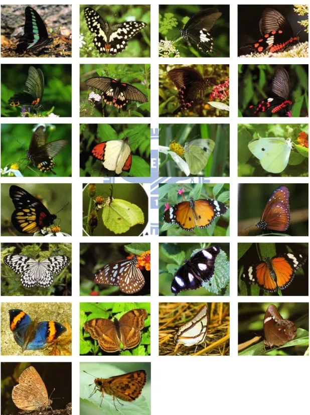
Fig. 1 The 26 species butterflies of image database . . . 8

Fig. 2 Three butterfly groups with similar appearances . . . 10

Fig. 3 Flow diagram of the proposed system . . . 13

Fig. 4 The natural image examples . . . 14

Fig. 5 Flow diagram of the segmentation steps . . . 15

Fig. 6 Example images of three cases . . . 18

Fig. 7 Two Sobel operators Gx and Gy . . . 19

Fig. 8 The step results of the segmentation method in clear case . . . 20

Fig. 9 The step results and comparison of the segmentation method in normal case . . . 23

Fig. 10 The result and comparison of the segmentation method in complex case . . . 25

Fig. 11 The ROI adjustment process . . . 26

Fig. 12 Flow diagram of the feature extraction steps . . . 28

Fig. 13 The system interfaces . . . 44

Fig. A.1 The example images of shooting direction . . . 49

vii

LIST OF TABLES

Table 1 The species of five (or six) butterfly categories . . . 9

Table 2 The initial weight of each feature in our database . . . 40

Table 3 The composition of three testing datasets . . . 42

Table 4 Performance on three testing datasets . . . 42

Table 5 The combing result of three testing datasets . . . .. . . 42

CHAPTER 1

INTRODUCTION

1.1 Motivation

While wandering around the field and forest, we are often impressed by many colorful butterflies around us. If people can easily obtain information of those butterflies, they will have more interest in understanding this beautiful creature and consequently the ecological preservation can be popularized. However, for ordinary people, without experts’ leading, it is hard for them to know the species of a butterfly. Even though they can consult a field guide or search on the Internet, the keyword choosing and the considerable searching time are still serious problems. Therefore, it would be greatly help if the butterfly can be recognized directly by its photographs taken from the outdoors.

1.2 Previous works

Although it has been almost ten years since the concept of butterfly image recognition was proposed, the research in this field is still limited. After searching plenty of literature, including IEEE, SCI, ACM and Google scholar, we only find less than 20 studies about butterfly recognition on “specimen image” and none of them are

on “natural image.” Therefore, in the following two sections, we first survey another nice paper about automatic segmentation on general images, and summarize the related works on butterfly recognition on “specimen image.”

1.2.1 Segmentation

Before recognition, there is a necessary step to extract the butterfly region from the background; however, the previous researches we found are all on specimen image. Since the background of nature image is much more complex than the simple and clear background in specimen image, the previous methods could not be applied to our situation. Therefore, we use the idea from another research about automatic segmentation on general images.

Li-Jen Chen and Ling-Hwei Chen [1] proposed a new fast method in automatic object segmentation based on human visual system. They first applied K-means on the local color distribution, the color values of all pixels, and obtained many small regions. Then, they analyzed the properties of each region: color composition, size, relative position, and coarseness. Finally, they used those color and texture properties to merge the similar regions. Although this research could achieve good results, it took too much computing time. Hence, we will only use the concept of its first step in our method.

1.2.2 Feature extraction and Recognition

The concept of butterfly image retrieval has been introduced around the late 1990s by Suzuki and Nagao [2-3]. At that time, due to the shortage of retrieval technology, the systems only supported text-based search. Recently, with the development of digital collection, biological image recognition has been noticed gradually. Some researchers started from the retrieval on butterfly specimen image [4-12].

During 2000 ~ 2003, Prof. Hsiang and his students [4-9] proposed a butterfly retrieval system on Internet and tried to retrieve the information from butterfly specimen image automatically. In 2000, they first built the retrieval system with all feature values given by human [4-5]. After the system construction, they discussed about the automaticity of object segmentation and color feature extraction. The correction rate of segmentation was 82%, and the best color feature they found was the human pre-defined perceptual level. Due to the unsatisfying results, they continued researching on automatic color and texture recognition on butterfly specimen image [6-9]. Nonetheless, their best recognition rate was about 50% measured by fuzzy average R-Precision, which evaluates the average R-Precision rate by counting the similar retrieval image as correct in some degree.

In 2002, Hyuga and Nishikawa [10] constructed a clustering system of butterfly

specimen image. They first calculated 88 features of each database image, including 10 color features of HSL color histogram, 26 shape features of local decimal and moment, 52 texture features of angular second moment, contrast, correlation and entropy. After that, they mapped all images to the Self-Organizing Maps (SOM) structure by their features, and divided them to clusters. The clustering results on the SOM map seemed disordered and overlapped seriously. Besides, the author did not support any experimental data.

In 2006, Lim [11] proposed the classification algorithm for butterfly and ladybug. The algorithm combined three traditional methods: morphology process, edge detection and color histogram. The author announced that this algorithm can recognize “every” insect (more than one) in an image taken on the field, and its average recognition ratio was extremely good, about 90%. Nevertheless, through our observation, its input and database images are all specimen images, and for each image, there is only one insect on it. This deviates from the author’s description. Besides, its database, consisting of 9 species of butterflies and 4 species of ladybugs, is insufficient for the reality.

In the later year, the lecture proposed by Starostenko [12] was closer to the real situation. This study could be divided into two parts, the shape indexing method and the feature filters. The indexing method [13], previously proposed for general image

retrieval, combined the SUSAN, CORPAI and 2STF algorithms. The later part included color, compactness and elongatedness features, and were used to pre-eliminate the butterfly species with large difference from the candidates. Its database consisted of 140 species and totally 1400 images, and for each species, the author defined its relevant degree with other species. Its average recall rate was 28%, and the average precision rate was 46%.

Considering the practicality for ordinary people and the further progress in this field, we propose a novel system for butterfly recognition on natural image. First, since there is no previous study on natural image, a useful database model is designed and constructed. Next, a user-friendly interactive segmentation method is provided to solve some problems on natural image. Then, the system can automatically extract the representative dominant colors of butterfly by the proposed Automatic Region Growing Boundary Thresholding (ARGBT) and Automatic Error Threshold K-means (AET-K-means) methods. The corresponding color and distribution features of each dominant color are acquired, and a similarity measurement is provided for recognition. After the recognition process, we also support two feedback mechanisms to come up to user’s expectation. Finally, the experimental results have shown the effectiveness of our system.

1.3 Organization of the thesis

This thesis is composed of five chapters. In Chapter 1, the motivation and previous works are introduced. Chapter 2 describes the butterfly images used in the study. The proposed recognition method is presented in Chapter 3. The experimental results and discussions are given in Chapter 4. Finally, the conclusion remarks in Chapter 5.

CHAPTER 2

LEPIDOPTERA IMAGE DATABASE

In this chapter, we will present the database in two different parts. The first section introduces the properties of our database. Then, based on the variety of natural butterfly images, we have designed a specialized database model in the second section.

2.1 Database introduction

Due to the passion and enthusiasm to our hometown, we choose the butterflies in Taiwan as our database. Considering the convenience of image acquirement and the visibility of ordinary people, our research focuses on Taiwanese common butterfly species. The butterfly image database was constructed of 26 common species shown in Fig. 1. According to the following three reasons, we can evidence that the amount of our database is sufficient and representative.

First, the species we collected can satisfy the requirement of a specified region. There are more than 400 species in Taiwan, and about 60~150 of them are defined as common species in different field guides. However, according to some experts’ observation, even in an area with rich butterfly sources, ordinary people usually find

only 5~15 common species during their trip. Hence, our database can satisfy reality condition.

Fig. 1. The 26 species butterflies of image database.

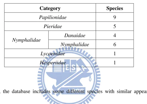
Next, from the view of biology, the variety of our database is adequate. As shown in Table1, based on the common classification in butterfly field, we collect at least one species for each category.

Table 1. The species of five (or six) butterfly categories

Category Species Papilionidae 9 Pieridae 5 Nymphalidae Danaidae 4 Nymphalidae 6 Lycaenidae 1 Hesperiidae 1

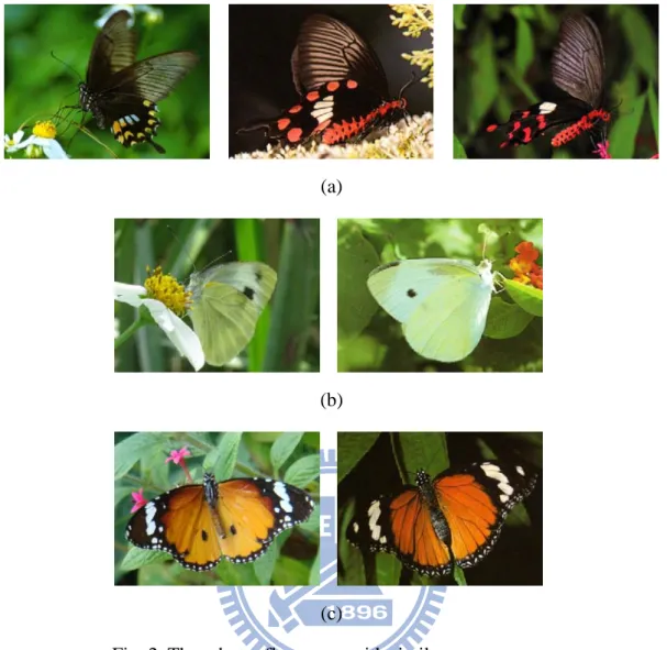
Third, the database includes some different species with similar appearances. Considering the experimental completeness and avoiding the testing bias, we collect three groups, shown in Fig. 2, whose members have similar appearances.

(a)

(b)

(c)

Fig. 2. Three butterfly groups with similar appearances.

2.2 Designed model

As our aim is to recognize butterfly images taken from various shooting directions and different butterfly postures in the real scene, under the consideration of database systemization and minimization, the design of database model is necessary. Therefore, we first analyze thousands of butterfly photographs on field guides [14-21] and internet, and field observation on live butterflies as well. After these works, considering the abilities of cell-phone camera and digital camera, we design the

model with 67 cases. These cases are taken from different wing-spreading angles and various shooting direction in both horizontal and vertical. In order to reduce the database size, each case is designed to cover maximum range of angle and decrease overlapping with each other. The detail of this model will be described in Appendix A. After the design, we face another problem that it is hard to take images of whole 67 cases for a live butterfly. Thanks for the helpful advice from the experts in The Insectarium of Taipei City Zoo; we use some complete corpses to simulate the poses of live butterfly and take pictures by mobile phone. Since the corpses are stiff and inflexible, it takes around 36~48 hours to soften 2~3 corpses, and then the simulation will cost at least 3~4 hours per corpse. In addition, because of the fragility of corpses, there is about 30% rate to fail the process, such as phosphor powder exfoliation and wings breakage. Therefore, the simulation process takes huge time and effort.

CHAPTER 3

PROPOSED METHOD

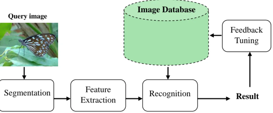
The flow diagram of the proposed system is shown in Fig. 3. The whole process consists of four major phases: segmentation, feature extraction, recognition and feedback. In the segmentation phase, through a friendly interactive interface user can easily choose the area containing the butterfly. With user’s help, the butterfly object, also known as the Region of Interest (ROI), can be roughly segmented from the natural image by our method. Next, in the feature extraction phase, after applying the proposed Automatic Region Growing Boundary Thresholding (ARGBT) and Automatic Error Threshold K-means (AET-K-means) methods, we can obtain the dominant colors of butterfly and extract the corresponding distribution features. In the recognition phase, a similarity measure is provided based on the extracted features. By using the similarity, the most related 20 images are determined, and user can obtain their species name and related information. Finally, in the feedback phase, two relevance feedback mechanisms are designed, one for the most related 20 images and the other for the most related image of each species. Through the feedback tuning process, our system can automatically adjust the feature weights and return new result which is closer to user’s expectation.

Fig. 3. Flow diagram of the proposed system. Feedback Tuning Image Database Result Query image Segmentation Feature Extraction Recognition

3.1 Segmentation

In this section, an interactive segmentation method will be described for butterfly boundary extraction on natural images. As mentioned in section 2.2.1, extracting the butterfly region from the background is a necessary step for following recognition. However, as for the segmentation on natural image, there is no previous research and many problems still exist. While taking pictures of butterfly in the field, we often encounter these kinds of situations: the butterfly is not at the center; the background is complex; the color of the butterfly is similar with the background and the butterfly might overlap with other object. Fig. 4 shows the example images of those situations. These problems make it difficult to extract the butterfly region from natural images automatically. Hence, an interactive segmentation method is provided to deal with

these issues. Steps of our method are shown in Fig. 5 and described below.

(a) (b)

(c) (d) Fig. 4. The natural image examples. (a) Butterfly not at the center. (b) With

complex background. (c) The butterfly in similar color with the background. (d) The butterfly overlapped with other object.

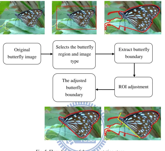
Selects the butterfly region and image

type Extract butterfly boundary Original butterfly image The adjusted butterfly boundary ROI adjustment

Fig. 5. Flow diagram of the segmentation steps.

3.1.1 Butterfly region and image type selection

In order to solve the problem of different butterfly positions and reduce the computation time, an interactive method is provided for user to select the butterfly region. First, a rectangle is drawn by user to select the region of interested butterfly using mouse click and drag. After this operation, user select the image type in the drawn rectangle. Due to different butterfly texture and background complexity, the input image can be divided into three cases:

Clear case :

There are three definitions of this case:

1. The pixels on butterfly boundary are all with strong edge response (high gradient magnitude).

2. The edge response of butterfly texture pixels are weaker than butterfly boundary.

3. The nearby background is unfocused or focused with a few edges connected with butterfly boundary.

Normal case :

There are three definitions of this case:

1. Most of the pixels on butterfly boundary are with strong edge response. (The colors of some pixels on butterfly boundary are similar with the connected background areas.)

2. The edge response of butterfly texture pixels may be stronger than the butterfly boundary.

3. The nearby background is focused with some edges connected with the butterfly boundary.

Complex case :

There are three definitions of this case:

1. Some pixels on the butterfly boundary are with strong edge response. (The colors of many pixels on butterfly boundary are similar with the connected background areas.)

2. The edge response of the butterfly texture pixels may be stronger than the butterfly boundary.

3. The nearby background is focused with many and complex edges connected with the butterfly boundary.

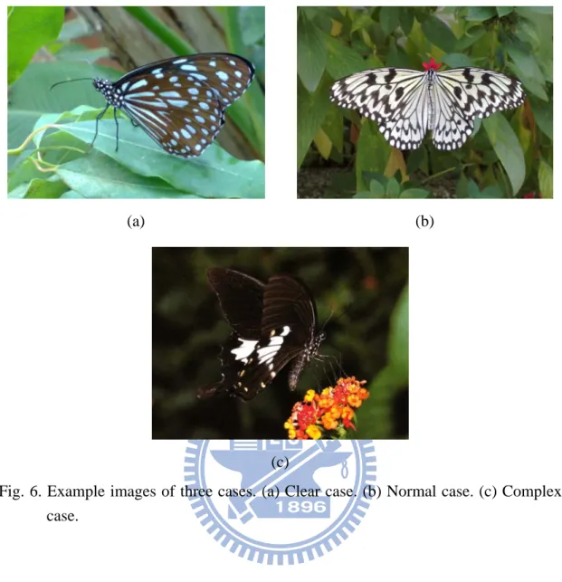
The example images of the three cases are shown in Fig. 6 Different segmentation methods will be applied to the corresponding image type and will be presented in the next step.

(a) (b)

(c)

Fig. 6. Example images of three cases. (a) Clear case. (b) Normal case. (c) Complex case.

3.1.2 Butterfly boundary extraction

The three different segmentation methods will be described as following:

Clear case:

Since the pixels of butterfly boundary have stronger edge response than the butterfly texture and nearby background, the boundary can fully enclose the butterfly. The extracting boundary steps of clear case are as follows, and the results of some

steps are shown in Fig. 8.

Step 1. Edge detection

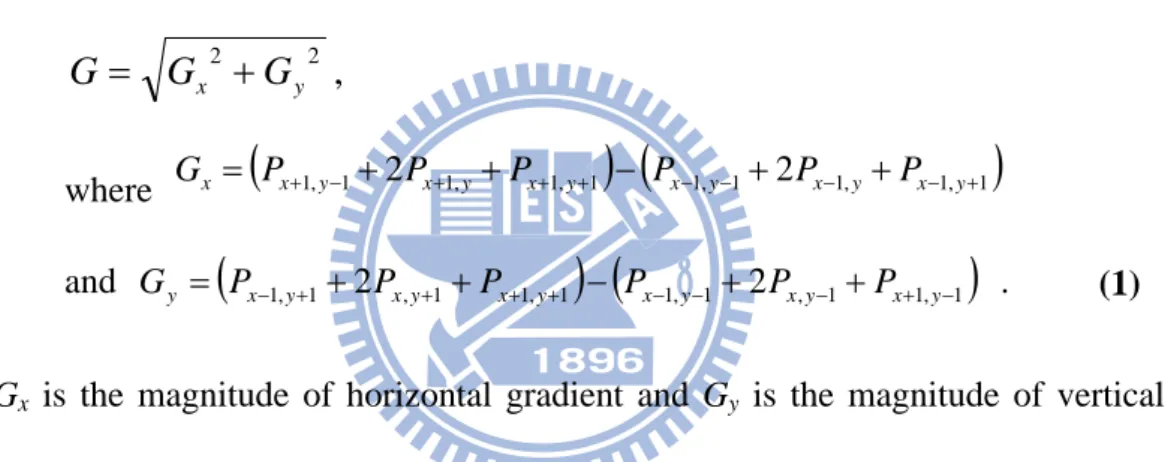
For all pixels in the drawn rectangle, compute the gradient magnitude of each pixel for each RGB channel, and calculate the maximum to produce the single-valued gradient magnitude image shown in Fig. 8(b). The gradient magnitude can be obtained by Sobel operators (see Fig. 7). The approximation of the magnitude G for pixel P_x,y is defined as

, 2 2 y x G G G = + where Gx =

(

) (

)

(

) (

)

Gx is the magnitude of horizontal gradient and Gy is the magnitude of vertical

gradient.

-1 0 1

-2 0 2

-1 0 1

-1 -2 -1

0 0 0

1 2 1

Fig. 7. Two Sobel operators Gx and Gy

(a) (b)

(c) (d)

(e) (f) Fig. 8. The step results of the segmentation method in clear case. (a) The original

image in the drawn rectangle. (b)-(e) Results of steps 1, 4, 5 and 6. (f) The extracted boundary.

Step 2. Otsu algorithm

Apply Otsu’s method [22] on the gradient image to acquire the Otsu value as edge threshold T1.

Step 3. Compute the cumulative distribution function (cdf) of the gradient image.

Step 4. Edge thresholding

Use the smooth region percentage P1 to find the corresponding value from the gradient cdf, as the edge threshold T2. Then, pick the smaller one among T1 and T2 to binarize the magnitude image. P1 will be adjusted by step 7, and its initial value will be set as 80%, which is usually the smooth region percentage we observed. The thresholding result of the final adjusted threshold is shown in Fig. 8(c).

Step 5. Fill the background and find the ROI.

Since the drawn rectangle covers the boundary, we can use the drawn rectangle as starting points to fill the background area. In the binary edge image, the points with value 0 on the drawn rectangle will be set as the starting points. Set value 255 as the stopping threshold, and find the connected component of the starting points. The result will be the background, and the largest remaining area will be the ROI. The result is shown in Fig. 8(d), in which the white area is the ROI and the black area is the background.

Step 6. Erode the boundary.

Due to the effect of Sobel operators, our edge will be thicker than its actual

size. Hence, we apply the morphology erosion on the ROI. After the erosion, obtain the largest remaining area as current ROI. The result is shown in Fig. 8(e).

Step 7. Check ROI percentage.

Because the ROI is the main region in the drawn rectangle, the percentage of its area should not be too small. Therefore, if the percentage is too small, we will decrease the region percentage P1 used in step 4 and repeat steps 4-7.

The final result of the segmentation method in clear case is shown in Fig. 8(f).

Normal case:

Since the colors of some pixels on butterfly boundary are in similar colors with the connected background areas, these pixels will have smaller gradient magnitude. These similar pixels will become the broken parts in the binary edge image; hence, we can use the morphology methods to repair the broken part and obtain the ROI. The steps are as listed below, and the results of some steps are shown in Fig. 9.

Step 1-4. The same as the steps 1-4 in clear case. The result of these steps is displayed in Fig. 9(b).

(a) (b)

(c) (d)

(e) (f)

(g) (h) Fig. 9. The step results and comparison of the segmentation method in normal case.

(a) The original image in the drawn rectangle. (b)-(f) Results of steps 4-9. (g) The extracted boundary. (h) The misusing result.

Step 5. Thicken the edges

Since the broken part need to be repaired, we apply the morphology dilation

on the edge image for several times. The result is shown in Fig. 9(c).

Step 6. The same as the step5 in clear case. Fig. 9(d) shows the result.

Step 7. Erode the boundary to remove the braches.

In recent ROI, there are two kinds of branches we need to remove. The background branches are produced by the edges connected to the butterfly boundary from the background. The branches of butterfly are the antennas and feet, which take smaller area and may be less important. In order to separate those branches, we can use the morphology erosion on the ROI for several times and keep the largest remaining area as the new ROI. Fig. 9(e) displays the result.

Step 8. The same as the step7 in clear case

Step 9. Remove regions connected and similar to the drawn rectangle.

After the morphology erosions in step 7, there might be some background areas which cannot be fully removed and are still connected with the drawn rectangle. To remove those areas, first apply the ARGBT algorithm (described in 3.2.1.1) to obtain the appropriate region growing boundary threshold. Next, set the points on the drawn rectangle as the starting points, and then find the connected components of the them by the region growing boundary threshold. Finally, we remove the result components, which belong to background, and

keep the largest remaining area as the new ROI. The result is shown in Fig. 9(f).

The final result of the segmentation method in normal case is shown in Fig. 9(g). Fig. 9(h) shows the bad result of misusing the segmentation method in clear case to this image.

Complex case:

The situation in complex case is similar with the normal case, except for the plenty strong variations in background or more pixels on boundary similar with backgound. Hence, we can apply the method in normal case without its last step. The result of the segmentation method in this case is shown in Fig. 10(b). Fig. 10(c) shows the bad result of misusing the segmentation method in normal case to this image.

(a) (b) (c) Fig. 10. The result and comparison of the segmentation method in complex case.

(a) The original image in the drawn rectangle. (b) The extracted boundary. (c) The comparison of the misusing result.

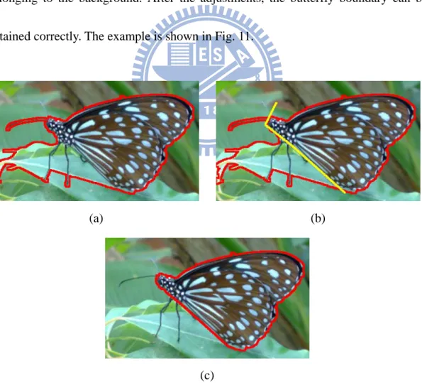
3.1.3 ROI adjustment

After the boundary extraction, there may be some “miss regions” and some “wrong regions” need user’s adjustment. The “miss regions” are the regions should belong to the butterfly; on the other hand, the “wrong regions” are the ones should belong to the background. By connecting the lines between different click points, user can easily draw lines by using mouse clicks. These lines can be used to add the “miss regions” back to the butterfly, or can be used to separate the “wrong regions” belonging to the background. After the adjustments, the butterfly boundary can be obtained correctly. The example is shown in Fig. 11.

(a) (b)

(c)

Fig. 11. The ROI adjustment process. (a) The original image in the drawn rectangle. (b) User draws lines to seperate the “wrong regions”. (c) The final segmentation result.

3.2 Feature extraction

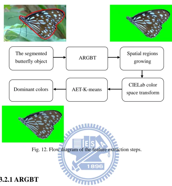
In the extracting process, since the number of dominant colors varies by different shooting cases and butterfly species, the AET-K-means method is proposed. The AET-K-means can automatically decide the proper number of dominant colors, and use the original K-means method to obtain those representative dominant colors. However, the number of the original colors of butterflies is a huge amount. If we just use this large amount of colors in K-means, it will cost more than 10 minutes to process only one resized image. Considering the extensive process time, by the concept from [1], we first merge the similar nearby pixels into small regions to reduce the number of input colors. The merging threshold is automatically decided by the proposed ARGBT method. Fig. 12 shows the flow diagram of extraction process.

Fig. 12. Flow diagram of the feature extraction steps.

ARGBT Spatial regions growing The segmented

butterfly object

AET-K-means CIELab color space transform Dominant colors

3.2.1 ARGBT

The ARGBT is used to automatically decide the region growing boundary threshold in the next section. Since the growing region can be thought as a smooth region and its boundary can be thought as the edges, ARGBT uses the smooth region percentage to obtain the corresponding values as the threshold. The steps are listed below

Step 1. Edge detection

Apply the same process as the step1 of clear case in 3.1.2, except the

butterfly contour pixels. Since we want to analyze the texture complexity of the butterfly, the butterfly contour pixels should be removed to avoid affecting the result.

Step 2. Calculate the smooth area percentage by Otsu algorithm.

By applying Otsu’s algorithm on the edge detection result, we can obtain an Otsu value as the threshold of binarization. Then we accumulate the pixel probabilities under the Otsu value. The accumulated result will be the smooth area percentage.

Step 3. Calculate the difference to the neighbor pixels.

For each pixel in the butterfly object, calculate the difference to each of its 8-way neighbors. The difference D from pixel to its neighbor is defined as y x

P

P

)

,

(

P

P

dis

P

P

D

−

=

where denotes the spatial distance from to . We compute the difference for each R, G, B channels, and the total difference by L2 metrics. Hence, four difference diagrams can be obtained in this step.

) , (P_x,y P_x,y dis i i

P

Step 4. Obtain four cumulative distribution functions (cdfs) of four difference diagrams.

Step 5. Decide the region growing boundary threshold.

By the smooth area percentage, we can obtain its corresponding value on each of the four cdfs. These values are defined as the region growing boundary threshold.

3.2.2 Spatial regions growing

By our statistics, there are tens of thousands of original colors of butterflies in a resized 400x300 image. If we just use this large amount of colors in the following K-means method, it will cost more than 10 minutes to process one resized image. In order to conserve the important spatial information of colors and to reduce the number of input colors in the following AET-K-means method, we first gather the nearby object pixels with similar colors into small regions. The connected component method is used for the region growing process, and the stopping threshold is the region growing boundary threshold. Since the average color is the representative for each region, if the region meets a new point, we will calculate four color differences to the average color in R, G, B channel, and the total difference by L2 metrics. If any of these differences is above the threshold, the new point will be set as the boundary.

After the process, the number of colors will be reduced to hundreds of colors and the process of the K-means can speed up for more than 1000 times. Besides, this

method also conserves the spatial information of the dominant colors. If we directly apply K-means algorithm on the original colors, it will just cluster similar colors into groups without considering the spatial information. For instance, a region with slightly different colors might be separated into different groups with other unrelated regions. Then, the spatial information of the region will be lost.

3.2.3 CIELab color space transform

Although the RGB color space is suitable for merging nearby pixels, it is perceptually non-linear to human vision system. Therefore, we transform RGB color space into CIELab color space [23] based on ITU-R Recommendation BT.709 with the D65 white point reference:

⎥ ⎥ ⎥ ⎦ ⎤ ⎢ ⎢ ⎢ ⎣ ⎡ ⎥ ⎥ ⎥ ⎦ ⎤ ⎢ ⎢ ⎢ ⎣ ⎡ = ⎥ ⎥ ⎥ ⎦ ⎤ ⎢ ⎢ ⎢ ⎣ ⎡ B G R Z Y X 950227 . 0 119193 . 0 019334 . 0 072169 . 0 715160 . 0 212671 . 0 180423 . 0 357580 . 0 412453 . 0 ' ' ' (3)

⎪

⎩

⎪

⎨

⎧

=

=

=

088754

.

1

/

'

000000

.

1

/

'

950456

.

0

/

'

Z

Z

Y

Y

X

X

⎟⎟

⎠

⎞

⎜⎜

⎝

⎛

−

⋅

=

500

*

X

Y

a

⎟⎟

⎠

⎞

⎜⎜

⎝

⎛

−

⋅

=

200

*

Y

Z

b

3.2.4 AET-K-means

After transforming the average color of each component to CIELab color space, we can apply the AET-K-Means on these colors. Traditional K-means has a significant drawback; the value of K must be decided initially and cannot be adjusted with different image. Hence, we utilize the concept from [1]: using an “error threshold” to decide the suitable K. The error in our method is defined to be the color difference between original color and the result center color of K-means. When these K colors cannot present the original colors, the average error will be larger than the error threshold. Then we should increase the value of K and repeat K-means algorithm. The process will finish only when the error is under the threshold, which means the result K colors can replace original colors within acceptable difference. By the observation of different shooting conditions of butterfly, the initial K value is 2 in our method, and the maximum value of K is 10. The error threshold is defined to be 10% of the color bandwidth, which is the range between the maximum and the minimum of a color channel. After the step, the final result colors will be the dominant colors of a

butterfly.

3.2.5 Color Features

The dominant colors are represented in CIELab color space in order to fit human vision system better and to acquire linearity during calculations. For each dominant color, there are three most important characteristics: CIELab values, area percentage of butterfly object, and its distribution properties. Besides color value and area percentage, for the distribution property, we choose six representative distribution properties as our color features. Hence, for mth dominant color of image i, its 8 color features will be

i m C m F1 2

: the CIELab color values of the dominant color, m

F : the area percentage of points belongs to the dominant color, m

F₃ : the distribution property 1, the ratio of the number of disconnected regions belonging to the dominant color. The function is

i i m m

N

N

F

=

: the number of disconnected regions belonging to the dominant color

i

N : the total number of disconnected regions of the butterfly

m

F4 : the distribution property 2, the ratio of the “average virtual radius.” The

function is

(

) (

)

(

) (

)

max

1

g

y

g

x

g

y

g

x

S

D

D

F

−

+

−

−

+

−

=

=

∑

: the average distance to the dominant color’s gravity center i

D : the maximum distance from the points of butterfly contour to its gravity center

i m

S : the number of points belonging to the dominant color

(

)

g _, , _, : the dominant color’s gravity center

(

)

y i x g

g , : the butterfly object’s gravity center

m

F₅ : the distribution property 3, the ratio of the dominant color’s center position. The function is

(

) (

)

D

g

g

g

g

F

−

+

−

=

D : the maximum distance from the points of butterfly contour to its gravity center

(

)

g _, , _, : the dominant color’s gravity center

(

)

y i x g

g , : the butterfly object’s gravity center

m

F₆ : the distribution property 4, the sharpness ratio. For each point belong to the dominant color, we calculate the distance from it to its gravity center. Then, the feature is computed as

90 10 6

R

R

F

=

R10: the average of the top one-tenth of the shortest distance

R90 : the average of the top one-tenth of the largest distance

m

F₇ : the distribution property 5, the standard deviation of disconnected region area size ratio. The function is

(

)

N

R

R

F

∑

−

=

Rt : the area size ratio of the tth disconnected region belonging to the

dominant color

R

i m

N

: the number of disconnected regions belonging to the dominant color

m

F₈ : the distribution property 6, the ratio of the convex-hall area. The

function is all con m

Aera

Aera

F

=

Aera

all

Aera

These features not only contain both color and spatial information, but also reveal the details of butterfly.

3.3 Recognition

Because of the variation of butterfly, a classification method is not used for grouping the different cases of a species of butterfly. For example, some cases of one species of Papilionidae might look much more similar with other species of Papilionidae, instead of itself. Hence, recognition is accomplished by the k-nearest neighbor algorithm.

In the k-nearest neighbor algorithm, each butterfly image is considered as an individual class. First, the system calculates the distance between the query image and all butterfly images in database. Since the color features are obtained from each

dominant color, we need to define the dominant color distance beforehand. The distance between two dominant colors Cm and Cn is calculated by Euclidean distance

(

)

_∑

−

=

,

C

f

f

C

d

where denotes the kth feature of dominant color Cm, denotes the kth feature

of dominant color Cn. Then, as for the image distance, while the numbers of dominant

colors varies by different butterfly images, a new distance function is provided. The distance between the database image i with M dominant colors and the query image q with N dominant colors will be

m k f fkn (14) (15)

( )

(

)

(

)

10

,

1

,

1

,

1

,

min

min

≤

≤

+

=

∑

∑

N

M

C

C

d

N

C

C

d

M

q

i

d

where denotes the mth dominant color of database image i, and denotes the nth dominant color of query image q.

i m

C Cnq

Finally, the recognition system ranks the distances and returns the top 20 nearest neighbors to the user. These returned images are called candidates.

3.4 Feedback

Since the result does not always meet the user’s expectation, two feedback

mechanisms are provided to adjust the weights of features in response to each user’s subjective point of view. The two mechanisms use the same relevance feedback algorithm to different candidates, which are the top 20 nearest neighbors and the nearest neighbor of each species respectively.

Our features are based on the dominant color; hence, the relevance feedback algorithm is especially designed for this property. The steps of our algorithm are presented as follows:

Step 1. User chooses u alike butterfly images, A1, A2, …, Au, and t unlike

butterfly images, N1, N2, …, Nt, from candidates.

Step 2. By previous similarity function, we can obtain the difference between a candidate image and the query image. Hence, for each alike image, calculate the difference produced by the kth feature. Summarize the differences D_kalike and obtain its percentage P_kalike, as follows:

8

...,

,

2

,

1

,

=

=

∑

k

D

D

P

Step 3. Repeat step2 on unlike images to obtain its percentage P_kunlike.

Step 4. Use the current kth feature weight wk to obtain the new weightwknew

8

...,

,

2

,

1

,

1

.

0

9

.

0

_⎟⎟

=

⎠

⎞

⎜⎜

⎝

⎛

×

+

=

k

P

P

w

w

As user’s expectation, these alike images should be similar with the query image, and the unlike images would be dissimilar with the query image. Therefore, for the kth feature, if is smaller than , which means the feature can represent the similarity relation correctly and whose weight should be increased. On the other hand, if is larger than , which means the feature cannot represent the similarity relation well and whose weight should be decreased. During the revising process, the weight will be adjusted smoothly since we multiply the original weight with higher percentage in order to keep the system stable. After adjusting these weights, the new result will be closer to what the user anticipates.

alike k P P_kunlike alike k P P_kunlike 39

CHAPTER 4

EXPERIMETAL RESULTS

In this chapter, experiments are conducted to evaluate the performance of our system. First, the separability of each feature is showed and will be used as our initial feature weight. Next, the three testing datasets will be introduced. Their related recognition results and discussions will also be revealed. Finally, the system’s interfaces and the feedback mechanisms will be shown.

Before the experiments start, the initial feature weights should be acquired first. We take one feature each time in recognition and receive the top 1 accuracy rate of each feature. Top 1 accuracy means that the first candidate is the same species of the query one. Then, the separability of each feature can be obtained, shown in Table 2, and the initial feature weights can be decided also.

Table 2. The initial weight of each feature in our database. Feature Top 1(%) Accuracy /

Initial weight Feature

Top 1(%) Accuracy / Initial weight F1 0.2378 F5 0.0747 F2 0.0853 F6 0.0558 F3 0.0564 F7 0.0865 F4 0.0744 F8 0.0904 40

The recognition results are presented based on three testing datasets. The three datasets are constructed by the sample images, the natural images from field guides and the natural images from internet. In the sample testing dataset, the images are taken in the simulation condition as the database images, but on different butterfly (partial) or under different shooting direction and light environment. In order to test each case of the designed model, we take two sample images for each case, and there will be total 3484 images in the sample testing set.

As for the natural images, due to different life cycle and habitats, we could not collect clear images of all kinds of butterflies by ourselves. To overcome this shortage, we obtain the natural images from field guides [14-20] as our field guide testing dataset. The field guide testing set includes 26 species and total 130 images. At the same time, we also acquire the natural images from internet as our network testing dataset. The network testing dataset includes 26 species and 60 images of each species. The details of three datasets are shown in Table 3. (These images are only used in this study for academic purpose, and will not be spread or be used in other way. Therefore, the copyright is not infringed. Besides, all images shown in this paper are either taken by ourselves, or obtained from the field guides [14-20].)

The result of three testing datasets is shown in Table 4. The average processing time is 8.71 seconds including user interaction and boundary segmentation time.

Table 3. The composition of three testing datasets.

Testing dataset Number of species Number of images Sample testing dataset 26 3484 Field guide testing dataset 26 130

Network testing dataset 26 1560

Table 4. Performance on three testing datasets. Testing dataset Recognition rate (%)

Top 1 Top 3 Top 5 Top 10 Top 20 Sample testing dataset 94.72 98.54 99.54 99.91 99.97 Field guide testing dataset 41.54 54.62 60.00 70.77 77.69 Network testing dataset 46.92 64.23 71.54 79.74 86.86

Considering the effect of three butterfly groups with similar appearances, we do the experiment again by combining each group as a species. The combining result shown in Table 5 is better in some degree than the original result, which means our method can solve part of the similarity problem.

Table 5. The combing result of three testing datasets. Testing dataset Recognition rate (%)

Top 1 Top 3 Top 5 Top 10 Top 20 Sample testing dataset 94.72 98.54 99.54 99.91 99.97 Field guide testing dataset 48.46 59.23 63.85 73.08 79.23 Network testing dataset 52.24 67.56 74.29 81.54 87.50

We have built our system on a PC by Java language. The system interfaces are shown in Fig. 13. Fig. 13(a) is the segmentation interface with user’s interactive operations, and Fig. 13(b) is the result interface which shows the top 20 candidate images after recognition. Fig. 13(b) also provides the first feedback mechanism. Through simple operations, user can choose the alike and unlike candidates easily, and the feature weights will be adjusted automatically. Another feedback mechanism for the most related candidate of each species is shown in Fig. 13(c). This mechanism provides another way to help user find the query species. As shown in Fig. 13(d), user can obtain clear butterfly images and the related information (Chinese name, English name, scientific name, family and other useful information) from a candidate by simply click on that image. Therefore, the system only needs one image in the retrieval results to be the correct species of the query one.

(a)

(b)

Fig. 13. The system interfaces. (a) Segmentation interface. (b) Recognition interface with the 1st feedback mechanism. (c) The 2nd feedback mechanism interface. (d) The related information of the chosen candidate image. (continued.)

(c)

(d)

Fig. 13. The system interfaces. (a) Segmentation interface. (b) Recognition interface with the 1st feedback mechanism. (c) The 2nd feedback mechanism interface. (d) The related information of the chosen candidate image.

CHAPTER 5

CONCLUTIONS

In the thesis, we have proposed an interactive method for butterfly recognition on natural image. First, the study designs and constructs the useful database model of natural butterfly images. This concept and related research have not been revealed yet. Second, a simple user interactive segmentation method is provided. The method is designed for the problems on natural images, which has been known as a challenging work for a long period. After segmentation, the system automatically extracts the dominant colors by the provided ARGBT and AET-K-means methods. Then, eight corresponding color and distribution features of each dominant color are obtained. In the end, a similarity measure is provided for recognition. Besides, to make the recognition result more close to the user’s requirement, two relevance feedback mechanisms are provided to automatically determine the importance of each feature. We hope our system can give more contribution to the related researches, and popularize the education of ecology protection well.

The system may be improved in the future from two aspects: the application on mobile devices and the further better features. The concept of popularizing ecological education of butterfly through mobile system and internet has been gradually revealed

with time. [24-25] introduced the mobile system application which helps students learn ecological knowledge and promote the academic work. [26-28] were the butterpree and analyses of Prof. Hsiang’s system [4]. [29] described virtual butterfly museum through internet, which provide a web-learning environment. From these researches, we can realize that if our system can be applied on the mobile devices, it will help greatly on both convenience and the ecological education popularization.

Besides current features, we can increase our features in two ways as the future work too. The first one is combining other features, which lead to nice results in other researches. The second one is considering the suitable shape and texture features for butterfly recognition. We have researched on some texture features, but have not obtained satisfying results yet. We hope these methods can improve our system, and maybe one day makes the world a better place.

APPENDIX A

The detail of the designed database model

In Table A.1, the wing-spreading angle is the angle between two wings of butterfly. As the butterfly spreads wings, the angle will increase from 0 to 180, which mean the close condition and the fully spread condition respectively. The angles of shooting direction can be explained by the 3-D diagram shown in Fig. A.1(a). The horizontal angle α means the angle at x-y plane, and the vertical angle β represents the angle along z-axis. We set the left side of butterfly (see Fig. A.1(b)) as angle 0 of the x-y plane, and set the horizontal, on which the butterfly is placed, as angle 0 along the z-axis. Besides, the shooting cases which are taken from the top (β = 90) or the bottom (β = -90) of butterfly will be recorded in their notations. As for the case description, we will not take pictures for the unused case, which is marked by the symbol “X”. The unused case is unnecessary for the database since its picture is similar with other cases or cannot give us enough information to recognize its species. The reason of each unused case will be recorded in notation. Finally, for the consultation convenience, the example images of whole 67 cases are shown in Fig. A.2.

㎏

(a) (b) Fig. A.1 The example images of shooting direction. (a) The 3-D diagram of

shooting direction. (b) The left side example image.

Table A.1. The detail of the designed database model. (continued)

Wing-spreading Angle Shooting Direction Case Number Notation Horizontal Angle Vertical Angle 0 0 0 001 180 0 002 20~40 0 45 003 0 X Similar with 001 (-10) 0 004 (10) 0 005 0 -45 X Similar with 001 45 45 006 0 007 -45 008 90 45 X Insufficient Information 0 X Insufficient Information -45 X Insufficient Information 135 45 009 0 010 -45 011 180 45 012 0 X Similar with 002 (170) 0 013 (190) 0 014 180 -45 X Similar with 002 49

Table A.1. The detail of the designed database model. (continued) Wing-spreading Angle Shooting Direction Case Number Notation Horizontal Angle Vertical Angle 20~40 225 45 015 0 016 -45 017 270 45 X Insufficient Information 0 X Insufficient Information -45 X Insufficient Information 315 45 018 0 019 -45 020 90 021 Top 50~70 0 45 022 0 X Insufficient Information -45 X Similar with 001 45 45 023 0 024 -45 025 90 45 X Insufficient Information 0 X Insufficient Information -45 X Insufficient Information 135 45 026 0 027 -45 028 180 45 029 0 X Insufficient Information -45 X Similar with 002 225 45 030 0 031 -45 032 270 45 X Insufficient Information 0 X Insufficient Information -45 X Insufficient Information 315 45 033 0 034 -45 035 90 036 Top 50

Table A.1. The detail of the designed database model. (continued) Wing-spreading Angle Shooting Direction Case Number Notation Horizontal Angle Vertical Angle 90~120 0 45 037 0 038 -45 X Similar with 001 45 45 039 0 040 -45 041 90 45 042 0 043 -45 X Insufficient Information 135 45 044 0 045 -45 046 180 45 047 0 048 -45 X Similar with 002 225 45 049 0 050 -45 051 270 45 052 0 X Insufficient Information -45 X Insufficient Information 315 45 053 0 054 -45 055 90 056 Top 160~180 0 45 057 0 X Insufficient Information -45 X Insufficient Information 45 45 058 0 X Insufficient Information -45 X Insufficient Information 90 45 059 0 X Insufficient Information -45 X Insufficient Information 51

Table A.1. The detail of the designed database model. Wing-spreading Angle Shooting Direction Case Number Notation Horizontal Angle Vertical Angle 160~180 135 45 060 0 X Insufficient Information -45 X Insufficient Information 180 45 061 0 X Insufficient Information -45 X Insufficient Information 225 45 062 0 X Insufficient Information -45 063 270 45 X Insufficient Information 0 X Insufficient Information -45 X Insufficient Information 315 45 064 0 X Insufficient Information -45 065 90 066 Top -90 067 Bottom

Fig. A.2. The example images of the 67 cases. (continued)

Fig. A.2. The example images of the 67 cases. (continued)

Fig. A.2. The example images of the 67 cases.

REFERENCES

[1] Li-Jen Chen, Ling-Hwei Chen, “A Fast Automatic Segmentation Algorithm based on Local Color-Distribution,” Master Thesis, Institute of Multimedia and Engineering, National Chiao Tung University, Taiwan, ROC, 2007.

[2] M. Nagao, K. Suzuki, A. Muraki, H. Ikeda, Y. Shimodaira, M. Yamazaki, “Retrieval of Butterfly from Its Sketched Image Utilizing Image Navigation Directory on Multimedia Network,” Proc. IEEE ICECS’98, Vol. 2, pp. 95-98, Sep. 1998.

[3] K. Suzuki, M. Nagao, A. Muraki, H. Ikeda, Y. Shimodaira, M. Yamazaki, “Reduction of Processing Time in Distributed Image Database System Utilizing Directory,” IEEE ICCT’98, Vol. 12, No. 7, pp. 629–639, Oct. 1998.

[4] J. Hong, H. Chen, J. Hsiang, “A Digital Museum of Taiwanese Butterflies,” Proceedings of the fifth ACM conference on Digital libraries, pp. 260-261, 2000. [5] B. Chen, J. Hsiang, “Content-Based Image Retrieval of Butterflies,” Master Thesis,

Department of Computer Science and Information Engineering, National Taiwan University, Taiwan, ROC, 2000.

[6] S. Lai, J. Hsiang, “Color Retrieval of Butterfly Images,” Master Thesis,

Department of Computer Science and Information Engineering, National Taiwan University, Taiwan, ROC, 2002.

[7] C. Hung, J. Hsiang, “Texture Retrieval of Butterfly Images,” Master Thesis, Department of Computer Science and Information Engineering, National Taiwan University, Taiwan, ROC, 2002.

[8] T. Huang, J. Hsiang, “MPEG-7 Based Butterfly Image Retrieval on Shape,” Master Thesis, Department of Computer Science and Information Engineering, National Taiwan University, Taiwan, ROC, 2002.

[9] W. Liu, J. Hsiang, “Model, Implementation, and Experiments for Fine-grained Image Retrieval,” Master Thesis, Department of Computer Science and Information Engineering, National Taiwan University, Taiwan, ROC, 2003.

[10] T. Hyuga, I. Nishikawa, “Implementing the Database System of Butterfly Specimen Image by Self-Organizing Maps,” Journal of Japan Society for Fuzzy Theory and Systems, Vol. 14, No. 1, pp. 74-81, 2002.

[11] J. Lim, J. Cho, T. Nam, S. Kim, “Development of A Classification Algorithm for Butterflies and Ladybugs,” 2006 IEEE Region 10 Conference TENCON 2006, pp. 1-3, Nov. 2006.

[12] O. Starostenko, C. K. Cruz, A. Chávez-Aragon, R. Contreras, “A Novel Shape Indexing Method for Automatic Classification of Lepidoptera”, XVII Int. Conf. on

Electronics, Communications, and Computers, Publ. IEEE Computer Society, pp.1-6, Feb. 2007.

[13] O. Starostenko, J. Chávez-Aragón, J. Sánchez, et al, “An Hybrid Approach for Image Retrieval with Ontological Content-Based Indexing,” Progress in pattern recognition, image analysis and applications, Springer-Verlag, Germany, Vol. 3773, pp. 997-1004, 2005.

[14] Y. Chang, “陽明山國家公園---賞蝶篇(上/下、導覽),” Yangmingshan National Park, Taiwan, 1994.

[15] The Forestry Bureau of Council of Agriculture Executive Yuan, “雙流蝶影,” The Forestry Bureau of Council of Agriculture Executive Yuan, Taiwan, 1998.

[16] Society of Wildlife And Nature, “愛蝴蝶護台灣,” Society of Wildlife And Nature, Taiwan, 1999.

[17] Y. Chang, “台灣賞蝶圖鑑,” Morning Star, Taiwan, 2000. [18] Y. Chang, “台灣賞蝶地圖,” Morning Star, Taiwan, 2002.

[19] Butterfly Conservation Society of Taiwan, “台灣常見的蝴蝶,” Taiwan, 2003. [20] Y. Chang, “蝴蝶100：台灣常見100種蝴蝶野外觀察及生活史全紀錄,”

Yuan-Liou, Taiwan, 2007.

[21] E. Hamano, Ecological Encyclopedia of TAIWANESE BUTTERFLIES, Japan 1986.

[22] N. Otsu, “A Threshold Selection Method from Gray-level Histogram,” IEEE Transactions on Systems, Man, Cybernetics 8, Vol. 9, pp. 62-66,1978.

[23] D. Margulis, “Photoshop Lab Color: The Canyon Conundrum and Other Adventures in the Most Powerful Colorspace,” Peachpit Press, 2005.

[24] Y. Chen, T. Kao, G. Yu, J. Sheu, “A Mobile Butterfly-Watching Learning System for Supporting Independent Learning,” Proceedings of the 2nd IEEE International Workshop on Wireless and Mobile Technologies in Education (WMTE'04), pp. 11-18, 2004.

[25] Y Yu, J. A. Stamberger, A. Manoharan, A. Paepcke, “EcoPod: A Mobile Tool for Community Based Biodiversity Collection Building,” In: Proceedings of the 6th ACM/IEEE-CS JCDL, pp. 344–353. Chapel Hill, NC, 2006.

[26] C. Yu, J. Hsiang, “Butterpree-Preparing Course Material from a Digital Museum of Butterflies,” Master Thesis, Department of Computer Science and Information Engineering, National Taiwan University, Taiwan, ROC, 2000.

[27] P. Wu, L. Chan, “The Evaluation of the Design of Web-based Learning Environment--A Case Study of Butterfly Digital Museum,” Master Thesis, Graduate Institute of Library & Information Science, National Chung Hsing University, Taiwan, ROC, 2002.

[28] S. Chen, J. Hsiang, “A System for Creating Course Material from a Digital

59

Museum,” Master Thesis, Department of Computer Science and Information Engineering, National Taiwan University, Taiwan, ROC, 2007.

[29] S. Chen, J. Hsiang, “Development of Internet Virtual Butterfly Museum,” Proc. of Int. Conf. on Computers in Education (ICCE’02), Vol. 2, pp. 1139-1143, 2002.