CROSS-REFERENCE MAXIMUM LIKELIHOOD ESTIMATE RECONSTRUCTION FOR POSITRON EMISSION TOMOGRAPHY

(1)

CROSS-REFERENCE MAXIMUM LIKELIHOOD

ESTIMATE RECONSTRUCTION FOR POSITRON

EMISSION TOMOGRAPHY

CHUNG-MING CHEN, HENRY HORNG-SHING Lu*, AND YUN-Pal Hsu*

Institute of Biomedical Engineering , National Taiwan University , Taipei,

*Institute of Statistics , National Chiao Tung University , Hsinchu , Taiwan , R.O.C.

Ma i i > ate (MLE) is a wia

fir, k hss been X&' wn t rWcOrtstrrxcting e

rs n &resrtlt Ia iu^ia`e anti cis.

md te,. i# e , opos, a ruw and rJj cM',U _met

€e str4eture 114 on. 3v, ;FI m, "skies, fl near Xe ing rived' arti 9 to the

ay o be correct, a the in

m is Culled c ' cross->Iie `^ liketiha

;r t

rp ry J

mpro `rââ t dr jè

Carle studies,

ut_al

, c.cer-i s ttse

_P

Wry or a ro, a t y

i> i t +^or

However, since the filtered -backprojection algorithms

were originally designed for X-ray Cr, many

assump-tions made for these algorithms do not hold for PET

image reconstruction . As a result , the reconstructed

images, especially those with small features , may not

be accurate enough for clinical use [1].

To overcome the potential problems inherent in

the filtered -backprojection algorithm, various ap-proaches based on maximum likelihood with EM al-gorithms have been proposed for PET image recon-struction , e.g., Shepp and Vardi [2], Lange and Carson

[3], Vardi, Shepp and Kaufman [4], Politte and Snyder [5], Fessler et al. [6]. Theoretically, the physical proc-ess of a PET system may be modeled as a Poisson

ran-dom process that suggests the ranran-dom observations in

a PET as Poisson random variables . Moreover, the

mean of these random variables is indirectly related to

1. INTRODUCTION

Positron Emission Tomography (PET) is a

func-tional imaging modality providing biochemical,

physiological , and metabolic information in the human

body. Like X-ray CT, the distribution of

radioisotope-labeled chemicals may be estimated from the measured

gamma photon pairs through filtered -backprojection

algorithms as adopted by most commercial PET

sys-tems accredited to their computational

efficiency.

Received : July 7, 2001; accepted : July 30, 2001

Correspondence: Chung-Ming Chen, Institute of

Biomedical Engineering , National Taiwan University.

Taipei, Taiwan, R.O.C.

-32-ABSTRACT

Maximum likelihood estimate (MLE) is a widely used approach for PET image reconstruction.

However, it has been shown that reconstructing emission tomography based on MLE without regu-

larization would result in noise and edge artifacts. In the attempt to regularize the maximum likeli-

hood estimate, we propose a new and efficient method in this paper to incorporate the correlated but

possibly incomplete structure information which may be derived from expertise, PET systems or other

imaging modalities. A mean estimate smoothing the MLE locally within each region of interest is

derived according to the boundaries provided by the structure information. Since the boundaries

may not be correct, a penalized MLE using the mean estimate is sought. The resulting reconstruc-

tion is called a cross-reference maximum likelihood estimate (CRMLE). The CRMLE can be ob-

tained through a modified EM algorithm, which is computation and storage efficient. By borrowing

the strength from the correct portion of boundary information, the CRMLE is able to extract the use-

ful

information to improve reconstruction for different kinds

of

incomplete and incorrect boundaries

in Monte Carlo studies. The proposed CRMLE algorithm not only reduces the estimation errors,

but also preserves the correct boundaries. The penalty parameters can be selected through human

interactions or automatically data-driven methods, such as the generalized cross validation method.

Biomed Eng Appl Basis Comm, 2001 (August);

13:

190-198.

Key Words: Maximum likelihood estimate, generalized

EM

algorithm, regularization, generalized

cross-validation.

(2)

APPLICATIONS, BASIS & COMMUNICATIONS

the target image intensity by a linear transformation.

Under this model, there are at least two sources of

er-rors intrinsic in the reconstruction of PET images. One

is due to the random variation of Poisson random

vari-ables. This can be handled via the maximum likelihood

approach as attempted by [2-6]. A good review on

the MLE approaches may be found in the book by

Snyder and Miller [7].

The other source of error is caused by the ill-posedness in inverting the linear transformation. This can be managed by the regularization methods [8-10]. Snyder et al. [11] demonstrated that the MLE without regularization will show the noise and edge artifacts. Therefore, it is important to regularize MLE for a bet-ter reconstruction. A variety of regularization methods have been studied in literature, like the early stopping rule in Veklerov and Llacer [12], the method of sieves in Snyder and Miller [13], the Bayesian approaches with different kinds of priors in Hebert and Leahy [14], Green [15], Herman et al. [16], and so on. Ouyang et al. [17] proposed to use the correlated structure informa-tion as the prior informainforma-tion and obtain the Bayesian reconstruction of PET via the "weighted line site" method in their series of studies. While the correlated structure information contains more information about boundaries than the mathematical form of regulariza-tion does, the Bayesian reconstrucregulariza-tion needs more computational efforts than the MLE-EM approaches. Therefore, in this paper, we would like to investigate a new and efficient approach to integrate the correlated but incomplete structure information using the MLE-EM approach. The correlated boundary information is obtained from an expert, an informed audience or the same or other tomography systems such as transmis-sion PET, X-ray CT scan, and MRI. The intensities within the boundaries are not necessarily uniformly distributed. The proposed method, which is named as a cross-reference maximum likelihood estimate (CRMLE), has been shown to not only fully utilize the correlated structure information to obtain a better re-construction, but also retain the computational effi-ciency of the MLE-EM approach in contrast to the Bayesian approach.

This paper is organized as follows. The model of

PET, the ill-posedness, stability, and finite sample

be-haviors of MLE will be investigated in Section 2.

Because of these phenomena, we will also discuss

some versions of regularization based on the MLE in

Section 2. Via incorporating the information of local

smoothness, we can get better reconstruction images

after cross-referring the correlated information. This

new method, CRMLE, will be introduced in Section 3.

The implementation issues such as the influences and

selection rules of penalty parameters will be

investi-gated in Section 4. The implementation results and

discussions are also presented in this section.

Conclu-sions and future studies are provided in Section 5.

2. PEI' MODEL AND MLE BEHAVIOR

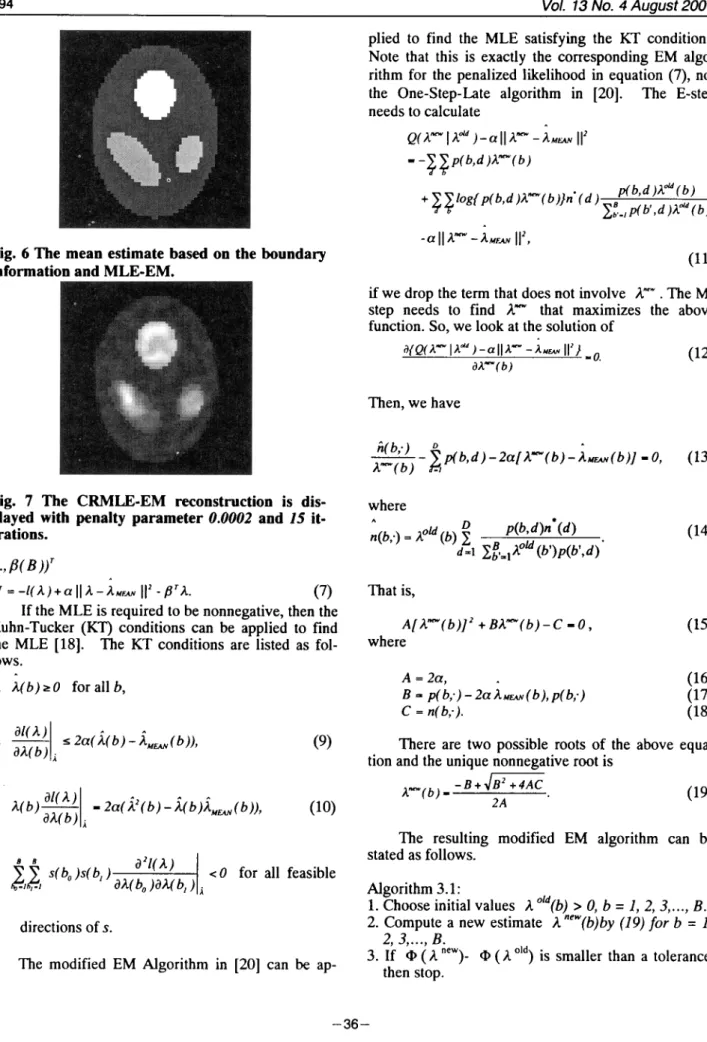
Consider the phantom illustrated Figure 1.

Sup-pose that there are three anatomic boundaries (ellipses)

that define three regions, each of which may be an

or-gan or a portion of a tissue. The emission intensity in

one region may be homogeneous within its boundary

as in the upper and right regions of Figure 1. That is,

the functional boundaries of emission intensities are

the same as the anatomic boundaries in the upper and

right regions. But, if some part of a region becomes

abnormal, the emission intensity will be

inhomogene-ous within the region as the left region of Figure 1.

The functional boundaries are thus different from the

anatomic boundaries. It is aimed to use the information

of anatomic boundaries to enhance the reconstructed

images without destroying the functional boundaries.

The model of the PET system employed in this studied follows that used in [2]. Let A denote the image to be reconstructed, which is decomposed into B square boxes (or pixels). The number of emission photon pairs generated in box b, n(b), is assumed to be Poisson distributed with a mean, A (b), for b = 1, 2, ..., B. Owing to the random variation of Poisson random variables, the actual number of emission, n(b), may be quite different from the mean, A (b). In par-ticular, for a large value of A (b), the variation is large since the variance of a Poisson random variable is equal to the mean.

When a positron radiates and annihilates with a nearby electron, two photons are generated and trav-eled in almost an opposite direction along a line. If two detectors within a preset time window receive these two photons, an ..annihilation event is identified in the tube formed by these two detectors. Let D denote the total number of tubes. For a PET system with Nd dis-tinct detectors, there can be at most (2d ) tubes.

Unlike the filtered-backprojection algorithms that

assume a space-invariant point spread function in

gen-eration of projection data, the "space-variant notion" is

incorporated in the PET model employed in this study

(3)

that may describe the physical process more closely.

Each box b is associated with a value, p(b, d), as the

probability for a pair of photons generated in the box b

and detected by the tube d, where b = 1, 2, ..., B and

d = 1, 2, ..., D.

One possible assignment for p(b, d)

would be the angle of view from box b to tube d.

Without loss of generality,

D

p(b,•) _ I p(b, d) is assumed to be 1.

d=1

According to the "thinning" property of Poisson

random variables [4,18], the total number of

coinci-dences detected by the d-th tube, n' (d) is an

inde-pendent Poisson random variable,

**n (d) - Poisson (A.* (d)),**

(1)

where '-' means 'distributed as,' and

* B

A (d) = I A(b)p(b, d)•

(2)

b=1

To see the performance of MLE in finite samples, Monte Carlo studies are simulated. Suppose the target phantom is as Figure 1. The number of boxes, B, is equal to Nb * Nb = 64*64 and the number of detectors is Nd = 64. The MLE can be reconstructed by the EM algorithm in Shepp and Vardi [2]. The log-likelihood of MLE-EM with respect to the iteration number is plotted in Figure 2. The log-likelihood is non-decreasing as the iteration number increases, which is assured by the property of EM algorithm. However, the log-likelihood of the true phantom is not the same as the converging value via the MLE-EM. At some iteration number, like 19 in this case study, the log-likelihood of MLE-EM would be closest to that of the true phantom. But as the iteration number increases further, the log-likelihood will be more and more away from that of the true phantom! To obtain the best reconstructed im-age before it deteriorates, Veklerov and Llacer [12] discussed the stopping rule based on statistical hy-pothesis testing. However, it is difficult to choose a proper stopping time in practice. Even if we select a good stopping time, such as 19 iterations in Figure 2, the reconstructed image in Figure 3 is still blurred without sharp boundaries and fine local structures. As the number of iterations increases, the reconstructed image becomes more and more blurring and spiky!

This is a commonplace phenomenon for MLE

approaches. Snyder et al. [11] showed that edge and

noise artifacts would be incurred due to the

ill-posedness of PET. A good alternative to reduce the

edge and noise artifacts is to use the regularization

methods. Several regularization methods have been

proposed previously. Silverman et al. [19] and Green

[20] added in a smoothness penalty in the

regulariza-tion method and modify the EM algorithm accordingly.

Snyder and Miller [13] used the method of sieves

to-gether with the EM algorithm. Green [15] also

consid-ered the modified EM algorithm for Bayesian

ap-proach with prior information about the patterns of

target images. In addition, the minimax estimator

based on tapered orthogonal series in Johnstone and

Silverman [21], the adaptive constrained methods of

regularization estimator in Lu and Wells [10] are also

proposed among many others.

To see the effects of regularization, a penalized MLE (PMLE) with a global penalty is demonstrated. Instead of maximizing the log-likelihood, one mini-mizes the negative value of log-likelihood and a 2-norm penalty. That is, this PMLE is

A

PMLE

= arg

minx{

-l(A) + allAII2 }, (3)

where 1( 2.) is the to -likelihood, a is a positive

pen-alty parameter and h All is the 2-norm of A. Ifa - 0 ,

then AC,u„., - A,,., On the other hand, if a - - , then

The penalty parameter, a, balances the

trade-off between the log-likelihood and the penalty term.

-EM

--- MLF.. 2 -- - --- - ----30 40 Snanm nuRlmr so 0

Fig. 2 The log-likelihoods of the MLE -EM, the

con-verging MLE, and the true phantom with respect to

the iteration numbers are displayed.

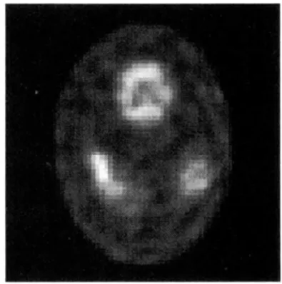
Fig. 3 The MLE-EM reconstruction is displayed

with 19 iterations.

(4)

-34-APPLICATIONS, BASIS & COMMUNICATIONS

The EM algorithm can be applied to find the

PMLE.

The updating formula becomes

-1 + 1 + 8an(b,.)

(4)

4a

where

b

_{X' b}

P(b,d)n(d)*

₍₅₎

n( ,.)_

(

)

g

, _,p(b,d)X (b )

Note that this is the unique nonnegative solution in the M step. The resulting estimates will be different for a different a. The log-likelihoods and 2-norm dif-ferences of MLE, PMLE and the true phantom can be plotted. If we choose a equal to the minimum value, 0.0001 in this case, then the PMLE has a less 2-norm difference with respect to the true phantom than that of the MLE. But the improvement is not too much as one can see that the PMLE in Figure 4 is about the same as the MLE in Figure 2. If the penalty a is chosen too large, then the PMLE will approach 0 and have even

Fig. 4 The PMLE-EM reconstruction is displayed

with penalty parameter 0.0001 and 19 iterations.

Fig. 5 The incomplete boundary information is

shown.

193

bigger 2-norm differences with respect to the true

phantom than those of the MLE. Therefore, the

se-lection of the penalty parameter is important.

The choice of penalty term is substantial as well.

Green [20] suggested another form of penalty form,

log {cosh(A(bo) - A(b, )} , where the sum is taken

over the neighboring pixel pairs. The resulting EM al-gorithm is difficult to obtain a closed form solution in the M-step. He proposed the One-Step-Late (OSL) al-gorithm that approximates the current solution via the previous solution in the M-step. These penalized terms can also be interpreted in the Bayesian framework. Geman and Geman [22] used the global energy func-tion with Gibbs sampling technique to obtain the Bayesian reconstruction. Ouyang et al. [17] tried to in-corporate the local smoothness contained in the boundaries to the Bayesian reconstruction by Gibbs samplings. In order to achieve this goal, they need to consider the energy function in the presence of line site induced by boundaries. While it is appealing in com-bining the local smoothness information, the computa-tion and complexity is quite demanding. In this paper, we propose a more efficient way to make use of the lo-cal structure as presented in the following section.

3. CROSS-REFERENCE MLE-EM

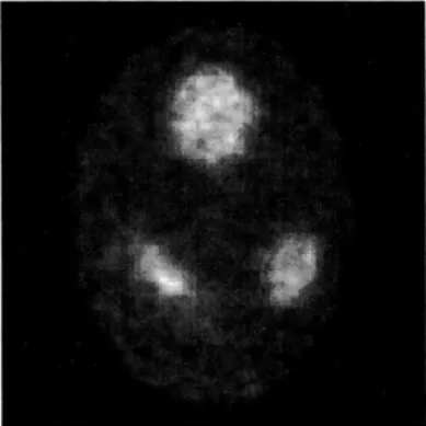
Since a boundary defines a region that is likely to have homogeneous emission intensities, we can get a mean estimate, AMF.AN , by doing the local average of the MLE within the boundaries. For instance, if the boundaries are as in Figure 5, the mean estimate is as Figure 6. However, the anatomical boundary may not be consistent with the functional boundary. That is, the boundary information may be incomplete. For example, the boundaries in Figure 5 do not contain all the boundaries in Figure 1. Thus, the mean estimate is only a rough estimate for the purpose of reference. In order to retain the local structure in the MLE, one needs to cross-refer the MLE and the mean estimate. Thus, we define the Cross-Reference MLE (CRMLE) as

AcRMLE = arg min,,, m(il) , (6) where

O(A)=-l(A)+aIIA-A. 112, (7) a > 0 and 2-norm is used for the penalty term. Suppose a - 0 _{, then A,RNLE - AMLE If a - - , then} A." - AMEAE • The resulting images by the CRMLE for one penalty parameter are shown in Figure 7. It is evident from Figure 7 that the CRMLE can borrow the strength from the local smoothness information via choosing a proper penalty parameter.

The Lagrangian function can be obtained after

in-troducing the Lagrangian multiplier , /3 = (/3(1), /3(2),

(5)

plied to find the MLE satisfying the KT conditions.

Note that this is exactly the corresponding EM

algo-rithm for the penalized likelihood in equation (7), not

the One-Step-Late algorithm in [20]. The E-step

needs to calculate

Q(A""" I e

)

- a llV - -AM 112

>p(b, d)A (b) +;;1og[ p(b,d)X-(b)}n (d) p( b,d)7^ d(b) ^e-,p(b',d)e

(b)

-a II A -AM

_IIz,

Fig. 6 The mean estimate based on the boundary

information and MLE-EM.

a{Q(A-I ) -aII

A'

-AMEAN

11

2"

0

.

(12)

al-(b) Then, we have n(b;) n b d 2 k- b A b 0 13 fi (b) - p( , ) - a[, ( ) - M&( )J = , ( ) where n(b,,) _ e' (b) 2 p(b,d)n*(d)

(14)

d=1 Xb-4A°"(b')p(b',d) That is, A[A"(b)] 2 +BA-(b)-C =0, (15)

where

A = 2a, .

(16)

B = p(b,) - 2a AME.,N (b), p(b,•) (17)

C=n(b;).

(18)

if we drop the term that does not involve A,

X" . The

M-step needs to find X- that maximizes the above

function . So, we look at the solution of

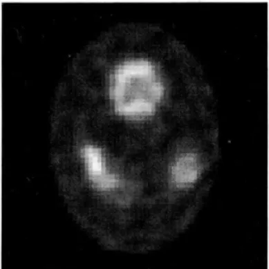
Fig. 7 The CRMLE -EM reconstruction is

dis-played with penalty parameter 0.0002 and 15

it-erations.

.... P(B ))T

W = -1(A) + a I I A- A.

I I2

- f T.t. (7)

If the MLE is required to be nonnegative , then the

Kuhn-Tucker (KT) conditions can be applied to find

the MLE [18].

The KT conditions are listed as

fol-lows.

1. A(b) Z0 forallb,

2 a1(A.)

al(b)

_z

s 2a(A(b) - AME,w (b)),

3. A(b) al(A) al(b)

4. S(bo )S(b,) al(bo

) aA(b, )

directions of s.

< 0 for all feasible

i

The modified EM Algorithm in [20] can be

ap-(9)

=2a(A2(b)-A(b)AM ( b)), (10)

x

a21(A)

There are two possible roots of the above

equa-tion and the unique nonnegative root is

(b)=-B+ B2+4AC 2A

(11)

(19)

The resulting modified EM algorithm can be

stated as follows.

Algorithm 3.1:

1. Choose initial values A "d(b) > 0, b = 1, 2, 3,..., B.

2. Compute a new estimate A "'(b)by (19) for b = 1,

2, 3,..., B.

3. If

1 (

A

new)_ (D

(

)old)

is smaller than a tolerance,

then stop.

(6)

Otherwise, go to step 2 with A old replaced by A new

The computation cost and complexity for the

pro-posed modified EM algorithm of CRMLE is of the same order as those of the MLE-EM. The convergence can be assured for any AMEAN because we only need to shift the origin to AMEAN and use the Proposition in Green [20]. Thus, the monotonic convergence also holds for the modified EM algorithm of CRMLE. That is, the computation advantages of the EM algo-rithm are intrinsic to the modified EM algoalgo-rithm in finding the CRMLE. The finite sample behaviors of CRMLE and the selection of penalty parameters are explored in the following section.

4. IMPLEMENTATION AND

DISCUSSIONS

In contrast to the selection of a good iteration number such that the log-likelihood of MLE-EM is close to that of the true phantom as in Figure 2 for the MLE-EM, the more crucial factor for the CRMLE is selection of the penalty parameter. The finite sample behaviors of CRMLE depend heavily on the choice of penalty parameters. The log-likelihood of the mean es-timate is usually smaller than those of the true phan-tom and MLE as one can see in Figure 8. This is be-cause the incomplete boundaries will oversmooth the image and pull down the log-likelihood to be below that of the true phantom. Since the log-likelihood of the true phantom lies somewhere in between those of MLE and mean estimate, it is reasonable to use the

log CRMLE --- log M ---- lag MEPN

--- log TRIE

mean estimate as a reference point in the framework of

MLE. As a - 0, the log-likelihood of CRMLE

will approach that of the MLE. But if a - oo , the

log-likelihood of the CRMLE will decrease to that of

the mean estimate. Thus, with a proper choice of a ,

the log-likelihood of CRMLE would be about the same

as that of the true phantom. If the discrepancy

meas-ure is changed from the log-likelihood differences to

the 2-norm differences with respect to the true

phan-tom, the influences of penalty parameters in terms of

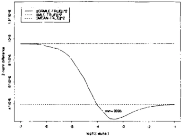
2-norm differences are shown in Figure 9. If the

pen-alty parameter is chosen in the neighborhood of

mini-mum point, 0.0005, the CRMLE can indeed beat the

mean estimate and MLE both numerically in Figure 9

and visually in Figure 7. The optimal values of a

may be slightly different in Figure 8 and 9 owing to

the difference of discrepancy measures.

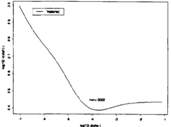
In practice, the true phantom is unknown and the optimal value of a is impossible to obtain from the plots in Figure 8 or 9. One may consider a dynamic graph function, such as a scrolling box or slider, to choose a proper a with user's interactions. Another way is to reroute to an automatically data-driven choice of penalty parameters. Leave-one-out cross-validation is one possible way. The idea is to remove one observation at a time. The remaining observations can be used to estimate the parameters. The fitted pa-rameters can be applied to predict the value that is omitted. The sum of prediction square errors would depend on the penalty parameters. The minimum value of the sum of prediction square errors can provide a suitable choice for the penalty parameters. This method can be generalized to the transformed model of

1=11--- --- ... ____ MN.1 LJE' 2

---

---d 1og70(,ipha ) 3 -2

Fig. 8 The log-likelihoods of the CRMLE-EM, the

converging MLE, the mean estimate and the true

phantom with respect to penalty parameters are

displayed.

---

__---__-n-.000.5

logt 0( Apha )

Fig. 9 The 2-norm differences of the CRMLE-EM,

the converging MLE, the mean estimate and the

true phantom with respect to penalty parameters

are displayed.

(7)

ridge regression such that the resulting choice of

pen-alty parameters is rotational invariant. This is called

as the generalized cross-validation (GCV) [23]. The

GCV function of the ridge estimate for the PET

recon-struction may be derived as

I

^^D Da z 2

V(a) = D r d, +Da) Z' (20) D

{D

_{d DDa}

+(D-D')1}:

where M = [p(b,d)]T, d, together with u;, i=1, 2, ..., D, are the eigenvalues and eigenvectors of MMT, D' is the rank of MMT, z, = u, y*, andy*(d) - n'(d)-y'ba(b,d) &,(b) The GCV function against the penalty parameters is plotted in Figure 10. The minimum value, 0.0002, is slightly different than the minimum values, 0.0005, in Figure 8 and 9. The CRMLE with a proper penalty pa-rameter selected in Figure 10 is shown in Figure 7. These two reconstructions do not differ too much in quality. If the boundary information is complete and correct, then the mean estimate will be a very good es-timate. However, if the boundary information is in-complete or incorrect, then the mean estimate will oversmooth and mask the local fine structures. Via the CRMLE with a proper penalty parameter, we can keep the local fine structures and make use of the boundary information at the same time . The resulting reconstruc-tion image in Figure 7 is very promising.

In calculating the GCV function, the eigenvalues

and eigenvectors of MMT are needed. The eigenvalue

or singular value decomposition (EVD or SVD) for a

matrix, symmetric or not, can be obtained by the

imsl_f_eig_sym or imsl_f_lin_svd_gen functions in

the IMSL C/MATH library for small- to medium-size

matrices. Due to the limit of hardware, the above

func-tion does not work for large-size matrices. The power

\ mn..066f

-6

"lot alo')

Fig. 10. The GCV curve with respect to penalty

parameters is drawn

method together with deflation [24] can be applied

then to obtain the EVD or SVD. The eigenvalues

ob-tained by the IMSL and power methods are not the

same. To check the correctness of these two

ap-proaches, we can plot the error of I MM T u; - d, u, I , in

2-norm, for all eigenvalues d, and eigenvectors u,. We

find that the IMSL function does not get the right EVD

at the beginning part and does a good job at the ending

part. The power method is on the contrary. Therefore,

if the leading part of EVD is needed, the power

method is proper. But if the ending part of EVD is

portant, then the IMSL method is suitable. An

im-proved numerical technique dominates the IMSL and

power methods will be certainly useful in order to find

the correct GCV. The EVD is quite computation

de-manding. But it is only needed to be done in one time

since the matrix M = [p(b,d)JT is fixed once the

con-figuration of PET system is set up.

If the boundaries are not only incomplete but also incorrect due to misalignment, the mean estimate will be even far away from the true phantom. However, the CRMLE can still pull out the useful information with unsharp boundaries for those incorrectly specified boundaries. That is, the CRMLE can distinguish the correctly and incorrectly specified boundaries auto-matically. For those correctly specified boundary in-formation, the CRMLE makes full use of the informa-tion because the mean estimate and MLE agree with each other. On the other hand, for the incorrect bound-ary information, the CRMLE recognizes the incorrect-ness and finds a good balance point between the mean estimate and MLE. If the boundaries are severely in-complete and incorrect, the mean estimate may even have larger 2-norm differences with respect to the true phantom than that of the MLE. The CRMLE can still outperform the MLE and the mean estimate. For in-stance, if the boundaries are so incomplete that there are only a half circle available in Figure 11, the mean estimate will lose the other half part of an ellipse.

Fig. 11. The incomplete boundary information is

shown.

(8)

Fig. 12 The CRMLE-EM reconstruction is

dis-played with penalty parameter 0.0003 and 15

itera-tions.

Fig. 13 Test phantom 2 is shown.

However, the CRMLE will make up the lost part as in Figure 12. The parameter, a = 0.0003, in Figure 12 is chosen because it minimizes both the GCV and 2-norm difference curves. The distinguished capability in extracting the useful portion of the severely incomplete and incorrect boundary information has been observed in many other experiments for CRMLE, which are not shown in this paper for succinctness. To see the above phenomena in a higher resolution, the number of boxes is raised to Nb * Nb = 128 * 128 and the number of de-tectors increases to Nd = 128. We also illustrate this in a different test phantom as in Figure 13. An extreme case is that we may have incomplete boundaries that have holes as in Figure 14. The boundaries may be in-correctly located as well. The mean estimate is quite far away from the test phantom 2 in Figure 15. For the parameter, a = 0.0005, that minimize the 2-norm differences, the reconstruction of CRMLE is shown in Figure 15. The CRMLE can even fill up the holes when the penalty parameter is small enough, say a

= 0.0002. In any case, the CRMLE is quite robust to

the misspecification and misalignment of boundaries. If the boundaries are complete and correct, then the mean estimate is a proper estimate. But if there is any doubt about the specification and alignment of boundaries, one shall use the CRMLE to reduce the

197

Fig. 14 The incomplete boundary information is

displayed.

Fig. 15 The CRMLE-EM reconstruction is

dis-played with penalty parameter 0.0005 and 10

itera-tions.

effects of misspecification and misalignment.

5. CONCLUSIONS AND FUTURE

WORKS

It has been shown in this study that the proposed CRMLE may take advantage of incomplete or incor-rect boundary information effectively. By introducing the penalty parameters, one can do the dedicatory bal-ance between the likelihood function and local smoothness within boundaries. By the modified EM algorithm derived, the computation speed and cost are of the same order as the MLE-EM. This makes the CRMLE-EM computationally feasible. Through either human interactions or the generalized cross-validation method, we can choose a suitable penalty parameter to do the fine tune-ups. The Monte Carlo studies demon-strate the improvements of the CRMLE over the MLE. While the simulation results have confirmed that the CRMLE is a very promising approach, further studies are definitely required to make this scheme clinically

(9)

applicable. Some important topics are how to register

the boundary information from other imaging modali-

ties on a PET, how to estimate the boundary if no other

imaging modality is available, how to select penalty

parameter more efficiently, etc. In addition, we would

like to apply the proposed CRMLE algorithm to the

real PET images as the next step.

ACKNOWLEDGMENTS

The authors would like to thank Professors I.-S.

Chang, C. A. Hsiung, B. M. W. Tsui and W. H. Wong

for their helpful discussions. This work was sup-

ported in part by the National Science Council of Tai-

wan, R. 0. C.

REFERENCES

1. Luo WA: Incorporating Sactial-Invariance Feature

in Filter-Backprojection Algorithms. Master Thesis,

National Taiwan University, 1996.

2. Shepp

LA

and Vardi Y: Maximum Likelihood Re-

construction for Emission Tomography. IEEE

Trans Med Imaging 1982;

1:

113-122.

3. Lange K and Carson R: EM Reconstruction Algo-

rithms for Emission and Transmission Tomography.

J Comput Assist Tomog 1984; 8: 306-316.

4. Vardi Y: Network Tomography

:

Estimating

Source-Destination Traffic Intensities from Link

Data. Journal of the American Statical Association

1996; 91(433): 365-377.

5.Politte DG and Snyder DL: Corrections for Acciden-

tal Coincidences and Attenuation in Maxirnum-

Likelihood Image Reconstruction for Positron-

Emission Tomography. IEEE Transactions. on

Medical Imaging 1991; lO(1): 82-89.

6. Fessler JA, Clinthorne NH and Rogers WL: On

Complete-Data Spaces for PET Reconstruction Al-

gorithms. IEEE Transactions on Nuclear Science

1993; 40(4): 1055-1061.

7. Snyder DL and Miller MI: Random Point Processes

in Time and Space. Springer,

znd

Ed., 1991.

8. Joyce LS and Root

'WL:

Precision Bounds in Sup-

perresolution Processing. J. Opt. Soc. Am. A 1983;

1: 149-168.

9. Lu HHS and Wells

MT: Minimax Theory for

La-

tent Function Estimation. Technical Report, Na-

tional Chiao Tung University, 1994.

10.Lu HHS and Wells

MT:

Adaptive Constrained

Method of Regularization Estimators for Latent

Density Estimation. Technical Report, National

Chiao Tung University, 1994.

11.Snyder DL, Miller MI, Thomas LIJ, and Politte DG:

Noise and Edge Artifacts in Maximum-Likelihood

Reconstructions for Emission Tomography. IEEE

Transactions on Medical Imaging 1987; 6: 228-238.

12.Veklerov

E and Llacer J: Stopping Rule for The

MLE Algorithm Based on StatisticalHypothesis

Testing. IEEE Trans. on Medical Imaging 1987;

6(4): 313-319.

13.Snyder DL and Miller MI: The Use of Sieves to

Stabilize Images Produced with The EM Algorithm

for Emission Tomography. IEEE Transactions on

Nuclear Science 1985; NS-32(5): 3864-3872.

14.Hebe1-t T and Leahy R: A Generalized EM Algo-

rithm for 3D Bayesian Reconstruction from Pois-

son Data Using Gibbs Priors. IEEE Trans. on

Medical Imaging 1989; 8(2): 194-202.

15. Green PJ: Bayesian Reconstructions from Emission

Tomography Data Using A Modified EM Algo-

rithm. IEEE Trans. Med. Imaging 1990; 9: 84-93.

16.Herman GT, Pierro ARD, and Gai N: On Methods

for Maximum A Posteriori Image Reconstruction

with A Normal Prior. Journal of Visual Communi-

cation and Image Representation 1992; 3(4): 316-

324. 17.0uyang X, Wong WH, Johnson VE, Hu X, and

Chen CT: Incorporation of Correlated Structural

Images in PET Image Reconstruction. IEEE Trans-

actions on Medical Imaging 1994; 13(4): 627-640.

18.Vardi Y, Shepp LA, and Kaufman L: A Statistical

Model for Positron Emission Tomography. Journal

of the American Statical Association 1985; 80: 8-

20. 19.Silverman BW, Jones MC, Wilson

JD, and Nychka

DW: A Smoothed EM Approach to Indirect Esti-

mation Problems, with Particular Reference to

Stereology and Emission Tomography. J. R. Statist.

SW. 1990; B-52(2): 271-324.

20.Green PJ: On Use of The EM Algorithm for Penal-

ized Likelihood Estimation. J. Roy. Statist. Soc.

1990; B-52(3): 453-467.

21.Johnstone IM and Silverman BW: Speed of

Estimation in Positron Emission Tomography and

251-280.

22.Geman S and Geman D: Stochastic Relaxation,

Gibbs Distribution, and The Bayesian Restoration

of Images. IEEE Trans. Pattern Anal. Machine In-

tell. 1984; 6: 721-740.

23.Golub GH, Heath M, and Wahba G: Generalized

Cross-Validation

As

A Method for Choosing A

Good Ridge Parameter. Tchnometrics 1979; 21(2):

215-223.

24.Parlett BN: The Symmetric Eigenvalue Problem.

Prentice-Hall, 1980.

applicable. Some important topics are how to register

the boundary information from other imaging

modali-ties on a PET, how to estimate the boundary if no other

imaging modality is available, how to select penalty

parameter more efficiently, etc. In addition, we would

like to apply the proposed CRMLE algorithm to the

real PET images as the next step.

ACKNOWLEDGMENTS

The authors would like to thank Professors I.-S.

Chang, C. A. Hsiung, B. M. W. Tsui and W. H. Wong

for their helpful discussions. This work was

sup-ported in part by the National Science Council of

Tai-wan, R. O. C.

REFERENCES

1. Luo WA: Incorporating Sactial-Invariance Feature

in Filter-Backprojection Algorithms. Master Thesis,

National Taiwan University, 1996.

2. Shepp LA and Vardi Y: Maximum Likelihood

Re-construction for Emission Tomography. IEEE

Trans Med Imaging 1982; 1: 113-122.

3. Lange K and Carson R: EM Reconstruction

Algo-rithms for Emission and Transmission Tomography.

J Comput Assist Tomog 1984; 8: 306-316.

4. Vardi Y: Network Tomography : Estimating

Source-Destination Traffic Intensities from Link

Data. Journal of the American Statical Association

1996; 91(433): 365-377.

5.Politte DG and Snyder DL: Corrections for

Acciden-tal Coincidences and Attenuation in

Maximum-Likelihood Image Reconstruction for

Positron-Emission Tomography. IEEE Transactions on

Medical Imaging 1991; 10(1): 82-89.

6. Fessler JA, Clinthome NH and Rogers WL: On

Complete-Data Spaces for PET Reconstruction

Al-gorithms. IEEE Transactions on Nuclear Science

1993; 40(4): 1055-1061.

7. Snyder DL and Miller MI: Random Point Processes

in Time and Space. Springer, 2"d Ed., 1991.

8. Joyce LS and Root WL: Precision Bounds in

Sup-perresolution Processing. J. Opt. Soc. Am. A 1983;

1: 149-168.

9. Lu HHS and Wells MT: Minimax Theory for

La-tent Function Estimation. Technical Report,

Na-tional Chiao Tung University, 1994.

10. Lu HHS and Wells MT: Adaptive Constrained

Method of Regularization Estimators for Latent

Density Estimation. Technical Report, National

Chiao Tung University, 1994.

11.Snyder DL, Miller MI, Thomas LJJ, and Politte DG:

Noise and Edge Artifacts in Maximum-Likelihood

Reconstructions for Emission Tomography. IEEE

Transactions on Medical Imaging 1987; 6: 228-238.

12.Veklerov E and Llacer J: Stopping Rule for The

MLE Algorithm Based on StatisticaiHypothesis

Testing. IEEE Trans. on Medical Imaging 1987;

6(4): 313-319.

13. Snyder DL and Miller MI: The Use of Sieves to

Stabilize Images Produced with The EM Algorithm

for Emission Tomography. IEEE Transactions on

Nuclear Science 1985; NS-32(5): 3864-3872.

14. Hebert T and Leahy R: A Generalized EM

Algo-rithm for 3D Bayesian Reconstruction from

Pois-son Data Using Gibbs Priors. IEEE Trans. on

Medical Imaging 1989; 8(2): 194-202.

15. Green PJ: Bayesian Reconstructions from Emission Tomography Data Using A Modified EM

Algo-rithm. IEEE Trans . Med. Imaging 1990; 9: 84-93.

16. Herman GT, Pierro ARD, and Gai N: On Methods for Maximum A Posteriori Image Reconstruction with A Normal Prior . Journal of Visual

Communi-cation and Image Representation 1992; 3(4):

316-324.

17. Ouyang X, Wong WH, Johnson VE, Hu X, and Chen Cr: Incorporation of Correlated Structural

Images in PET Image Reconstruction . IEEE Trans-actions on Medical Imaging 1994; 13(4): 627-640.