Amazon Timestream

(1)

Amazon Timestream

Developer Guide

(2)

Amazon Timestream: Developer Guide

Copyright © Amazon Web Services, Inc. and/or its aﬃliates. All rights reserved.

Amazon's trademarks and trade dress may not be used in connection with any product or service that is not Amazon's, in any manner that is likely to cause confusion among customers, or in any manner that disparages or discredits Amazon. All other trademarks not owned by Amazon are the property of their respective owners, who may or may not be aﬃliated with, connected to, or sponsored by Amazon.

(3)

What Is Amazon Timestream?

Amazon Timestream is a fast, scalable, fully managed, purpose-built time series database that makes it easy to store and analyze trillions of time series data points per day. Timestream saves you time and cost in managing the lifecycle of time series data by keeping recent data in memory and moving historical data to a cost optimized storage tier based upon user deﬁned policies. Timestream’s purpose-built query engine lets you access and analyze recent and historical data together, without having to specify its location. Amazon Timestream has built-in time series analytics functions, helping you identify trends and patterns in your data in near real-time. Timestream is serverless and automatically scales up or down to adjust capacity and performance. Because you don’t need to manage the underlying infrastructure, you can focus on optimizing and building your applications.

Timestream also integrates with commonly used services for data collection, visualization, and machine learning. You can send data to Amazon Timestream using AWS IoT Core, Amazon Kinesis, Amazon MSK, and open source Telegraf. You can visualize data using Amazon QuickSight, Grafana, and business intelligence tools through JDBC. You can also use Amazon SageMaker with Timestream for machine learning.

Topics

• Timestream Key Beneﬁts (p. 1)

• Timestream Use Cases (p. 2)

• Getting Started With Timestream (p. 2)

Timestream Key Beneﬁts

The key beneﬁts of Amazon Timestream are:

• Serverless with auto-scaling - With Amazon Timestream, there are no servers to manage and no capacity to provision. As the needs of your application change, Timestream automatically scales to adjust capacity.

• Data lifecycle management - Amazon Timestream simplifies the complex process of data lifecycle management. It offers storage tiering, with a memory store for recent data and a magnetic store for historical data. Amazon Timestream automates the transfer of data from the memory store to the magnetic store based upon user configurable policies.

• Simpliﬁed data access - With Amazon Timestream, you no longer need to use disparate tools to access recent and historical data. Amazon Timestream's purpose-built query engine transparently accesses and combines data across storage tiers without you having to specify the data location.

• Purpose-built for time series - You can quickly analyze time series data using SQL, with built-in time series functions for smoothing, approximation, and interpolation. Timestream also supports advanced aggregates, window functions, and complex data types such as arrays and rows.

• Always encrypted - Amazon Timestream ensures that your time series data is always encrypted, whether at rest or in transit. Amazon Timestream also enables you to specify an AWS KMS customer managed key (CMK) for encrypting data in the magnetic store.

• High availability - Amazon Timestream ensures high availability of your write and read requests by automatically replicating data and allocating resources across at least 3 diﬀerent Availability Zones within a single AWS Region. For more information, see the Timestream Service Level Agreement.

• Durability - Amazon Timestream ensures durability of your data by automatically replicating your memory and magnetic store data across diﬀerent Availability Zones within a single AWS Region. All of your data is written to disk before acknowledging your write request as complete.

(9)

Timestream Use Cases

Examples of a growing list of use cases for Timestream include:

• Monitoring metrics to improve the performance and availability of your applications.

• Storage and analysis of industrial telemetry to streamline equipment management and maintenance.

• Tracking user interaction with an application over time.

• Storage and analysis of IoT sensor data

Getting Started With Timestream

We recommend that you begin by reading the following sections:

• Tutorial (p. 99)- To create a database populated with sample data sets and run sample queries.

• Timestream Concepts (p. 3)-To learn essential Timestream concepts.

• Accessing Timestream (p. 84)-To learn how to access Timestream using the console, AWS CLI, or API.

• Quotas (p. 331)-To learn about quotas on the number of Timestream components that you can provision.

To learn how to quickly begin developing applications for Timestream, see the following:

• Using the AWS SDKs (p. 95)

• Query Language Reference (p. 273)

(10)

How It Works

The following sections provide an overview of Amazon Timestream service components and how they interact.

After you read this introduction, see the Accessing Timestream (p. 84) sections, to learn how to access Timestream using the Console, CLI or SDKs.

Topics

• Timestream Concepts (p. 3)

• Architecture (p. 4)

• Writes (p. 7)

• Storage (p. 15)

• Query (p. 16)

• Scheduled Query (p. 18)

Timestream Concepts

Time series data is a sequence of data points recorded over a time interval. This type of data is used for measuring events that change over time. Examples include:

• stock prices over time

• temperature measurements over time

• CPU utilization of an EC2 instance over time

With time series data, each data point consists of a timestamp, one or more attributes, and the event that changes over time. This data can be used to derive insights into the performance and health of an application, detect anomalies, and identify optimization opportunities. For example, DevOps engineers might want to view data that measures changes in infrastructure performance metrics. Manufacturers might want to track IoT sensor data that measures changes in equipment across a facility. Online marketers might want to analyze clickstream data that captures how a user navigates a website over time. Because time series data is generated from multiple sources in extremely high volumes, it needs to be cost-eﬀectively collected in near real time, and therefore requires eﬃcient storage that helps organize and analyze the data.

Following are the key concepts of Timestream:

• Time series - A sequence of one or more data points (or records) recorded over a time interval. Examples are the price of a stock over time, the CPU or memory utilization of an EC2 instance over time, and the temperature/pressure reading of an IoT sensor over time.

• Record - A single data point in a time series.

• Dimension - An attribute that describes the meta-data of a time series. A dimension consists of a dimension name and a dimension value. Consider the following examples:

• When considering a stock exchange as a dimension, the dimension name is "stock exchange" and the dimension value is "NYSE"

(11)

• When considering an AWS Region as a dimension, the dimension name is "region" and the dimension value is "us-east-1".

• For an IoT sensor, the dimension name is "device ID" and the dimension value is "12345"

• Measure - The actual value being measured by the record. Examples are the stock price, the CPU or memory utilization, and the temperature or humidity reading. Measures consist of measure names and measure values. Consider the following examples:

• For a stock price, the measure name is "stock price" and the measure value is the actual stock price at a point in time.

• For CPU utilization, the measure name is "CPU utilization" and the measure value is the actual CPU utilization.

• Timestamp - Indicates when a measure was collected for a given record. Timestream supports timestamps with nanosecond granularity.

• Table - A container for a set of related time series.

• Database - A top level container for tables.

A summary of Timestream Concepts

A database contains 0 or more tables. Each table contains 0 or more time series. Each time series consists of a sequence of records over a given time interval at a speciﬁed granularity. Each time series can be described using its meta-data or dimensions, its data or measures, and its timestamps.

Architecture

Amazon Timestream has been designed from the ground up to collect, store, and process time series data at scale. Its serverless architecture supports fully decoupled data ingestion, storage, and query processing systems that can scale independently. This design simpliﬁes each sub-system, making it easier to achieve unwavering reliability, eliminate scaling bottlenecks, and reduce the chances of correlated system failures. Each of these factors becomes more important as the system scales. You can read more about each topic below.

Topics

(12)

• Write Architecture (p. 5)

• Storage Architecture (p. 6)

• Query Architecture (p. 6)

• Cellular Architecture (p. 6)

Write Architecture

When writing time-series data Amazon Timestream routes writes for a table, partition, to a fault- tolerant memory store instance that processes high throughput data writes. The memory store in turn achieves durability in a separate storage system that replicates the data across three availability zones (AZs). Replication is quorum based such that the loss of nodes, or an entire AZ, will not disrupt write availability. In near real-time, other in-memory storage nodes sync to the data in order to serve queries.

The reader replica nodes span AZs as well, to ensure high read availability.

Timestream supports writing data directly into the magnetic store, for applications generating lower throughput late arrival data. Late arrival data is data with a timestamp earlier than the current time.

Similar to the high throughput writes in the memory store, the data written into the magnetic store is replicated across three AZs and the replication is quorum based.

Whether data is written to the memory or magnetic store, Timestream automatically indexes and partitions data before writing it to storage. A single Timestream table may have hundreds, thousands, or even millions of partitions. Individual partitions do not, directly, communicate with each other and do not share any data (shared-nothing architecture). Instead, the partitioning of a table is tracked through a highly available partition tracking and indexing service. This provides another separation of concerns designed speciﬁcally to minimize the eﬀect of failures in the system and make correlated failures much less likely.

(13)

Storage Architecture

When data is stored in Timestream data is organized in time order as well as across time based on context attributes written with the data. Having a partitioning scheme that divides “space” in addition to time is important for massively scaling a time series system. This is because most time series data is written at or around the current time. As a result, partitioning by time alone does not do a good job of distributing write traﬃc or allowing for eﬀective pruning of data at query time. This is important for extreme scale time series processing, and it has allowed Timestream to scale orders of magnitude higher than the other leading systems out there today in serverless fashion. The resulting partitions are refer to as “Tiles”, since they represent divisions of a two-dimensional space which are designed to be of similar size. Timestream tables start out as a single partition (tile), and then split in the spatial dimension as throughput requires. When tiles reach a certain size, they then split in the time dimension in order to achieve better read parallelism as the data size grows.

Timestream is designed to automatically manage the lifecycle of time series data. Timestream offers two data stores – an in-memory store and a cost-effective magnetic store, and it supports configuring table level policies to automatically transfer data across stores. Incoming high throughput data writes land in the memory store where data is optimized for writes, as well as reads performed around current time for powering dashboard and alerting type queries. When the main time-frame for writes, alerting, and dashboarding needs has passed, allowing the data to automatically flow from the memory store to the magnetic store to optimize cost. Timestream allows setting a data retention policy on the memory store for this purpose. Data writes for late arrival data are directly written into the magnetic store.

Once the data is available in the magnetic store (because of expiration of the memory store retention period or because of direct writes into the magnetic store), it is reorganized into a format that is highly optimized for large volume data reads. The magnetic store also has a data retention policy that may be configured if there is a time threshold where the data outlives its usefulness. When the data exceeds the time range defined for the magnetic store retention policy, it is automatically removed. Therefore, with Timestream, other than some configuration, the data lifecycle management occurs seamlessly behind the scenes.

Query Architecture

Timestream queries are expressed in a SQL grammar that has extensions for time series-speciﬁc support (time series-speciﬁc data types and functions), so the learning curve is easy for developers already familiar with SQL. Queries are then processed by an adaptive, distributed query engine that uses metadata from the tile tracking and indexing service to seamlessly access and combine data across data stores at the time the query is issued. This makes for an experience that resonates well with customers as it collapses many of the Rube Goldberg complexities into a simple and familiar database abstraction.

Queries are run by a dedicated fleet of workers where the number of workers enlisted to run a given query is determined by query complexity and data size. Performance for complex queries over large data sets is achieved through massive parallelism, both on the query execution fleet and the storage fleets of the system. The ability to analyze massive amounts of data quickly and efficiently is one of Timestream’s greatest strengths. A single query executing over terabytes or even petabytes of data may have thousands of machines working on it all at the same time.

Cellular Architecture

To ensure that Timestream can offer virtually infinite scale for your applications, while simultaneously ensuring 99.99% availability, the system is also designed using a cellular architecture. Rather than scaling the system as a whole, Timestream segments into multiple smaller copies of itself, referred to as cells. This allows cells to be tested at full scale, and prevents a system problem in one cell from affecting activity in any other cells in a given region. While Timestream is designed to support multiple cells per region, consider the following fictitious scenario, in which there are 2 cells in a region:

(14)

In the scenario depicted above, the data ingestion and query requests are ﬁrst processed by the discovery endpoint for data ingestion and query, respectively. Then, the discovery endpoint identiﬁes the cell containing the customer data, and directs the request to the appropriate ingestion or query endpoint for that cell. When using the SDKs, these endpoint management tasks are transparently handled for you.

Note

When using VPC Endpoints with Timestream or directly accessing REST APIs for Timestream, you will need to interact directly with the cellular endpoints. For guidance on how to do so, see VPC Endpoints (p. 240) for instructions on how to set up VPC Endpoints, and Endpoint Discovery Pattern (p. 93) for instructions on direct invocation of the REST APIs.

Writes

You can collect time series data from connected devices, IT systems, and industrial equipment, and write it into Timestream. Timestream enables you to write data points from a single time series and/or data points from many series in a single write request when the time series belong to the same table. For your convenience, Timestream oﬀers you with a ﬂexible schema that auto detects the column names and data types for your Timestream tables based on the dimension names and the data types of the measure values you specify when invoking writes into the database. You can also write batches of data into Timestream.

Timestream supports the following data types for writes:

Data type Description

BIGINT Represent a 64-bit integer.

BOOLEAN Represents the two truth values of logic, namely, true and false.

DOUBLE 64-bit variable-precision implementing the IEEE Standard 754 for Binary Floating-Point Arithmetic.

VARCHAR Variable length character data with an optional maximum length. The maximum limit is 2KB.

(15)

Data type Description

MULTI Data type for multi-measure records. This data type includes one or more measures of type BIGINT, BOOLEAN, DOUBLE, VARCHAR, and TIMESTAMP.

TIMESTAMP Represents an instance in time using nanosecond precision time in UTC, tracking the time since Unix time. This data type is currently supported only for multi-measure records (i.e. within measure values of type MULTI).

Note

Timestream supports eventual consistency semantics for reads. This means that when you query data immediately after writing a batch of data into Timestream, the query results might not reﬂect the results of a recently completed write operation. The results may also include some stale data. Similarly, while writing time series data with one or more new dimensions, a query can return a partial subset of columns for a short period of time. If you repeat theses query requests after a short time, the results should return the latest data.

You can write data using the AWS SDKs (p. 95), AWS CLI (p. 90), or through AWS Lambda (p. 245), AWS IoT Core (p. 247), Amazon Kinesis Data Analytics for Apache Flink (p. 250), Amazon

Kinesis (p. 251), Amazon MSK (p. 251) and Open source Telegraf (p. 256).

Topics

• No upfront schema deﬁnition (p. 8)

• Writing data (Inserts and Upserts) (p. 8)

• Batching writes (p. 15)

• Eventual consistency for reads (p. 15)

No upfront schema deﬁnition

Before sending data into Amazon Timestream, you must create a database and a table using the AWS Management Console, Timestream’s SDKs, or the Timestream APIs. For more information, see Create a database (p. 88) and Create a table (p. 88). While creating the table, you do not need to deﬁne

the schema up front. Amazon Timestream automatically detects the schema based on the measures and dimensions of the data points being sent, so you no longer need to alter your schema oﬄine to adapt it to your rapidly changing time series data.

Writing data (Inserts and Upserts)

The write operation in Amazon Timestream enables you to insert and upsert data. By default, writes in Amazon Timestream follow the first writer wins semantics, where data is stored as append only and duplicate records are rejected. While the first writer wins semantics satisfies the requirements of many time series applications, there are scenarios where applications need to update existing records in an idempotent manner and/or write data with the last writer wins semantics, where the record with the highest version is stored in the service. To address these scenarios, Amazon Timestream provides the ability to upsert data. Upsert is an operation that inserts a record in to the system when the record does not exist or updates the record, when one exists. When the record is updated, it is updated in an idempotent manner.

Writing data into the memory store and the magnetic store

Amazon Timestream oﬀers the ability to directly write data into the memory store and the magnetic store. The memory store is optimized for high throughput data writes and the magnetic store is

(16)

optimized for lower throughput writes of late arrival data. Late arrival data is data with a timestamp earlier than the current time. You must explicitly enable the ability to write late arrival data into the magnetic store by enabling magnetic store writes for the table.

Writing data with single-measure records and multi-measure records

Amazon Timestream oﬀers the ability to write data using two types of records, namely, single-measure records and multi-measure records.

Single-measure records

Single-measure records enable you to send a single measure per record. When data is sent to

Timestream using this format, Timestream creates one table row per record. This means that if a device emits 4 metrics and each metric is sent as a single-measure record, Timestream will create 4 rows in the table to store this data, and the device attributes will be repeated for each row. This format is recommended in cases when you want to monitor a single metric from an application or when your application does not emit multiple metrics at the same time.

Multi-measure records

With multi-measure records, you can store multiple measures in a single table row, instead of storing one measure per table row. Multi-measure records therefore enable you to migrate your existing data from relational databases to Amazon Timestream with minimal changes.

You can also batch more data in a single write request than single-measure records. This increases data write throughput and performance, and also reduces the cost of data writes. This is because batching more data in a write request enables Amazon Timestream to identify more repeatable data in a single write request (where applicable), and charge only once for repeated data.

Topics

• Multi-measure records (p. 9)

• Writing data with a timestamp that exists in the past or in the future (p. 14)

Multi-measure records

With multi-measure records, you can store your time-series data in a more compact format in the memory and magnetic store, which helps lower data storage costs. Also, the compact data storage lends itself to writing simpler queries for data retrieval, improves query performance, and lowers the cost of queries.

Furthermore, multi-measure records also support the TIMESTAMP data type for storing more than one timestamp in a time-series record. TIMESTAMP attributes in a multi-measure record support timestamps in future or past. Multi-measure records therefore help improve performance, cost, and query simplicity

—and offer more flexibility for storing different types of correlated measures.

Beneﬁts

The following are the beneﬁts of using multi-measure records:

• Performance and cost – Multi-measure records enable you to write multiple time-series measures in a single write request. This increases the write throughput and also reduces the cost of writes. With multi-measure records, you can store data in a more compact manner, which helps lower the data storage costs. The compact data storage of multi-measure records results in less data being processed by queries. This is designed to improve the overall query performance and help lower the query cost.

• Query simplicity – With multi-measure records, you do not need to write complex common table expressions (CTEs) in a query to read multiple measures with the same timestamp. This is because the

(17)

measures are stored as columns in a single table row. Multi-measure records therefore enable writing simpler queries.

• Data modeling ﬂexibility – You can write future timestamps into Timestream by using the

TIMESTAMP data type and multi-measure records. A multi-measure record can have multiple attributes of TIMESTAMP data type, in addition to the time ﬁeld in a record. TIMESTAMP attributes, in a multi- measure record, can have timestamps in the future or the past and behave like the time ﬁeld except that Timestream does not index on the values of type TIMESTAMP in a multi-measure record.

Use cases

You can use multi-measure records for any time-series application that generates more than one measurement from the same device at any given time. The following are some example applications:

• A video streaming platform that generates hundreds of metrics at a given time.

• Medical devices that generate measurements such as blood oxygen levels, heart rate, and pulse.

• Industrial equipment such as oil rigs that generate metrics, temperature, and weather sensors.

• Other applications that are architected with one or more microservices.

Example: Monitoring the performance and health of a video streaming application

Consider a video streaming application that is running on 200 EC2 instances. You want to use Amazon Timestream to store and analyze the metrics being emitted from the application, so you can understand the performance and health of your application, quickly identify anomalies, resolve issues, and discover optimization opportunities.

We will model this scenario with single-measure records and multi-measure records, and then compare/

contrast both approaches. For each approach, we make the following assumptions:

• Each EC2 instance emits four measures (video_startup_time, rebuﬀering_ratio,

video_playback_failures, and average_frame_rate) and four dimensions (device_id, device_type, os_version, and region) per second.

• You want to store 6 hours of data in the memory store and 6 months of data in the magnetic store.

• To identify anomalies, you’ve set up 10 queries that run every minute to identify any unusual activity over the past few minutes. You’ve also built a dashboard with eight widgets that display the last 6 hours of data, so that you can eﬀectively monitor your application. This dashboard is accessed by ﬁve users at any given time and is auto-refreshed every hour.

Using single measure records

Data modeling: With single measure records, we will create one record for each of the four measures (video startup time, rebuﬀering ratio, video playback failures, and average frame rate). Each record will have the four dimensions (device_id, device_type, os_version, and region) and a timestamp.

Writes:When you write data into Amazon Timestream, the records are constructed as follows:

public void writeRecords() {

System.out.println("Writing records");

// Specify repeated values for all records List<Record> records = new ArrayList<>();

final long time = System.currentTimeMillis();

List<Dimension> dimensions = new ArrayList<>();

final Dimension device_id = new

Dimension().withName("device_id").withValue("12345678");

(18)

final Dimension device_type = new

Dimension().withName("device_type").withValue("iPhone 11");

final Dimension os_version = new

Dimension().withName("os_version").withValue("14.8");

final Dimension region = new Dimension().withName("region").withValue("us-east-1");

dimensions.add(device_id);

dimensions.add(device_type);

dimensions.add(os_version);

dimensions.add(region);

Record videoStartupTime = new Record() .withDimensions(dimensions)

.withMeasureName("video_startup_time") .withMeasureValue("200")

.withMeasureValueType(MeasureValueType.BIGINT) .withTime(String.valueOf(time));

Record rebufferingRatio = new Record() .withDimensions(dimensions)

.withMeasureName("rebuffering_ratio") .withMeasureValue("0.5")

.withMeasureValueType(MeasureValueType.DOUBLE) .withTime(String.valueOf(time));

Record videoPlaybackFailures = new Record() .withDimensions(dimensions)

.withMeasureName("video_playback_failures") .withMeasureValue("0")

.withMeasureValueType(MeasureValueType.BIGINT) .withTime(String.valueOf(time));

Record averageFrameRate = new Record() .withDimensions(dimensions)

.withMeasureName("average_frame_rate") .withMeasureValue("0.5")

.withMeasureValueType(MeasureValueType.DOUBLE) .withTime(String.valueOf(time));

records.add(videoStartupTime);

records.add(rebufferingRatio);

records.add(videoPlaybackFailures);

records.add(averageFrameRate);

WriteRecordsRequest writeRecordsRequest = new WriteRecordsRequest() .withDatabaseName(DATABASE_NAME)

.withTableName(TABLE_NAME) .withRecords(records);

try {

WriteRecordsResult writeRecordsResult = amazonTimestreamWrite.writeRecords(writeRecordsRequest);

System.out.println("WriteRecords Status: " + writeRecordsResult.getSdkHttpMetadata().getHttpStatusCode());

} catch (RejectedRecordsException e) {

System.out.println("RejectedRecords: " + e);

for (RejectedRecord rejectedRecord : e.getRejectedRecords()) {

System.out.println("Rejected Index " + rejectedRecord.getRecordIndex() + ":

"

+ rejectedRecord.getReason());

}

System.out.println("Other records were written successfully. ");

} catch (Exception e) {

System.out.println("Error: " + e);

} }

When you store single-measure records, the data is logically represented as:

(19)

time device_id device_type os_version region measure_namemeasure_value::bigintmeasure_value::double 2021-09-07

21:48:44 .00000000012345678 iPhone 11 14.8 us-east-1 video_startup_time200 2021-09-07

21:48:44 .00000000012345678 iPhone 11 14.8 us-east-1 rebuﬀering_ratio 0.5 2021-09-07

21:48:44 .00000000012345678 iPhone 11 14.8 us-east-1 video_playback_failures0 2021-09-07

21:48:44 .00000000012345678 iPhone 11 14.8 us-east-1 average_frame_rate 0.85 2021-09-07

21:53:44 .00000000012345678 iPhone 11 14.8 us-east-1 video_startup_time500 2021-09-07

21:53:44 .00000000012345678 iPhone 11 14.8 us-east-1 rebuﬀering_ratio 1.5 2021-09-07

21:53:44 .00000000012345678 iPhone 11 14.8 us-east-1 video_playback_failures10 2021-09-07

21:53:44 .00000000012345678 iPhone 11 14.8 us-east-1 average_frame_rate 0.2

Queries: You can write a query that retrieves all of the data points with the same timestamp received over the past 15 minutes as:

with cte_video_startup_time as ( SELECT time, device_id, device_type, os_version, region, measure_value::bigint as video_startup_time FROM table where time >= ago(15m) and

measure_name=”video_startup_time”),

cte_rebuffering_ratio as ( SELECT time, device_id, device_type, os_version, region, measure_value::double as rebuffering_ratio FROM table where time >= ago(15m) and measure_name=”rebuffering_ratio”),

cte_video_playback_failures as ( SELECT time, device_id, device_type, os_version, region, measure_value::bigint as video_playback_failures FROM table where time >= ago(15m) and measure_name=”video_playback_failures”),

cte_average_frame_rate as ( SELECT time, device_id, device_type, os_version, region, measure_value::double as average_frame_rate FROM table where time >= ago(15m) and measure_name=”average_frame_rate”)

SELECT a.time, a.device_id, a.os_version, a.region, a.video_startup_time, b.rebuffering_ratio, c.video_playback_failures, d.average_frame_rate FROM cte_video_startup_time a, cte_buffering_ratio b, cte_video_playback_failures c, cte_average_frame_rate d WHERE

a.time = b.time AND a.device_id = b.device_id AND a.os_version = b.os_version AND a.region=b.region AND

a.time = c.time AND a.device_id = c.device_id AND a.os_version = c.os_version AND a.region=c.region AND

a.time = d.time AND a.device_id = d.device_id AND a.os_version = d.os_version AND a.region=d.region

Workload cost: The cost of this workload is estimated to be $373.23 per month with single-measure records

Using multi-measure records

Data modeling: : With multi-measure records, we will create one record that contains all four measures (video startup time, rebuﬀering ratio, video playback failures, and average frame rate), all four

dimensions (device_id, device_type, os_version, and region), and a timestamp.

(20)

Writes:When you write data into Amazon Timestream, the records are constructed as follows:

public void writeRecords() {

System.out.println("Writing records");

// Specify repeated values for all records List<Record> records = new ArrayList<>();

final long time = System.currentTimeMillis();

List<Dimension> dimensions = new ArrayList<>();

final Dimension device_id = new

Dimension().withName("device_id").withValue("12345678");

final Dimension device_type = new

Dimension().withName("device_type").withValue("iPhone 11");

final Dimension os_version = new

Dimension().withName("os_version").withValue("14.8");

final Dimension region = new Dimension().withName("region").withValue("us-east-1");

dimensions.add(device_id);

dimensions.add(device_type);

dimensions.add(os_version);

dimensions.add(region);

Record videoMetrics = new Record() .withDimensions(dimensions) .withMeasureName("video_metrics") .withTime(String.valueOf(time));

.withMeasureValueType(MeasureValueType.MULTI) .withMeasureValues(

new MeasureValue()

.withName("video_startup_time") .withValue("0")

.withValueType(MeasureValueType.BIGINT), new MeasureValue()

.withName("rebuffering_ratio") .withValue("0.5")

.withType(MeasureValueType.DOUBLE), new MeasureValue()

.withName("video_playback_failures") .withValue("0")

.withValueType(MeasureValueType.BIGINT), new MeasureValue()

.withName("average_frame_rate") .withValue("0.5")

.withValueType(MeasureValueType.DOUBLE)) records.add(videoMetrics);

WriteRecordsRequest writeRecordsRequest = new WriteRecordsRequest() .withDatabaseName(DATABASE_NAME)

.withTableName(TABLE_NAME) .withRecords(records);

try {

WriteRecordsResult writeRecordsResult = amazonTimestreamWrite.writeRecords(writeRecordsRequest);

System.out.println("WriteRecords Status: " + writeRecordsResult.getSdkHttpMetadata().getHttpStatusCode());

} catch (RejectedRecordsException e) {

System.out.println("RejectedRecords: " + e);

for (RejectedRecord rejectedRecord : e.getRejectedRecords()) {

System.out.println("Rejected Index " + rejectedRecord.getRecordIndex() + ":

"

+ rejectedRecord.getReason());

}

(21)

System.out.println("Other records were written successfully. ");

} catch (Exception e) {

System.out.println("Error: " + e);

} }

When you store multi-measure records, the data is logically represented as:

time device_id device_typeos_versionregion measure_namevideo_startup_timerebuﬀering_ratiovideo_

playback_failuresaverage_frame_rate 2021-09-07

21:48:44 .00000000012345678iPhone

11 14.8 us-

east-1 video_metrics200 0.5 0 0.85

2021-09-07

21:53:44 .00000000012345678iPhone

11 14.8 us-

east-1 video_metrics500 1.5 10 0.2

Queries: You can write a query that retrieves all of the data points with the same timestamp received over the past 15 minutes as:

SELECT time, device_id, device_type, os_version, region, video_startup_time,

rebuffering_ratio, video_playback_failures, average_frame_rate FROM table where time >=

ago(15m)

Workload cost: The cost of workload is estimated to be $127.43 with multi-measure records.

Note

In this case, using multi-measure records reduces the overall estimated monthly spend by 2.5x, with the data writes cost reduced by 3.3x, the storage cost reduced by 3.3x, and the query cost reduced by 1.2x.

Writing data with a timestamp that exists in the past or in the future

Timestream oﬀers the ability to write data with a timestamp that lies outside of the memory store retention window through a couple diﬀerent mechanisms.

• Magnetic store writes – You can write late arrival data directly into the magnetic store through magnetic store writes. To use magnetic store writes, you must ﬁrst enable magnetic store writes for a table. You can then ingest data into the table using the same mechanism used for writing data into the memory store. Amazon Timestream will automatically write the data into the magnetic store based on its timestamp.

Note

The write-to-read latency for the magnetic store can be up to 6 hours, unlike writing data into the memory store, where the write-to-read latency is in the sub-second range.

• TIMESTAMP datatype for measures – You can use the TIMESTAMP data type to store data from the past, present, or future. A multi-measure record can have multiple attributes of TIMESTAMP data type, in addition to the time ﬁeld in a record. TIMESTAMP attributes, in a multi-measure record, can have timestamps in the future or the past and behave like the time ﬁeld except that Timestream does not index on the values of type TIMESTAMP in a multi-measure record.

Note

The TIMESTAMP datatype is supported only for multi-measure records.

(22)

Batching writes

Amazon Timestream enables you to write data points from a single time series and/or data points from many series in a single write request. Batching multiple data points in a single write operation is beneﬁcial from a performance and cost perspective. See Writes (p. 325) in the Metering and Pricing section for more details.

Note

Your write requests to Timestream may be throttled as Timestream scales to adapt to the data ingestion needs of your application. If your applications encounter throttling exceptions, you must continue to send data at the same (or higher) throughput to allow Timestream to automatically scale to your application's needs.

Eventual consistency for reads

Timestream supports eventual consistency semantics for reads. This means that when you query data immediately after writing a batch of data into Timestream, the query results might not reﬂect the results of a recently completed write operation. If you repeat these query requests after a short time, the results should return the latest data.

Storage

Timestream stores and organizes your time series data to optimize query processing time and to reduce storage costs. It oﬀers data storage tiering and supports two storage tiers: a memory store and a magnetic store. The memory store is optimized for high throughput data writes and fast point-in-time queries. The magnetic store is optimized for lower throughput late arrival data writes, long term data storage, and fast analytical queries.

Timestream ensures durability of your data by automatically replicating your memory and magnetic store data across diﬀerent Availability Zones within a single AWS Region. All of your data is written to disk before acknowledging your write request as complete.

Timestream enables you to conﬁgure retention policies to move data from the memory store to the magnetic store. When the data reaches the conﬁgured value, Timestream automatically moves the data to the magnetic store. You can also set a retention value on the magnetic store. When data expires out of the magnetic store, it is permanently deleted

For example, consider a scenario where you conﬁgure the memory store to hold a week’s-worth of data and the magnetic store to hold 1 year’s-worth of data. The age of the data is computed using the timestamp associated with the data point. When the data in the memory store becomes a week old it is automatically moved to the magnetic store. It is then retained in the magnetic store for a year. When the data becomes a year old, it is deleted from Timestream. The retention values of the memory store and the magnetic store cumulatively deﬁne the amount of time your data will be stored in Timestream. This means that for the above scenario, from the time of data arrival, the data is stored in Timestream for a total period of 1 year and 1 week.

Note

When you upgrade the retention period of the memory or magnetic store, the retention change takes eﬀect from that point onwards. For example, if the retention period of the memory store was set to 2 hours and then changed to 24 hours by updating the table retention policies, the memory store will be capable of holding 24 hours of data, but will be populated with 24 hours of data 22 hours after this change was made. Timestream does not retrieve data from the magnetic store to populate the memory store.

To ensure the security of your time series data, your data in Timestream is always encrypted by default.

This applies to data in transit and at rest. Furthermore, Timestream enables you to use customer-

(23)

managed CMK keys to secure your data in the magnetic store. For more information on customer managed CMKs, see Customer master Keys.

Query

With Timestream, you can easily store and analyze metrics for DevOps, sensor data for IoT applications, and industrial telemetry data for equipment maintenance, as well as many other use cases. Timestream’s purpose-built, adaptive query engine allows you to access data across storage tiers using a single SQL statement. It transparently accesses and combines data across storage tiers without requiring you to specify the data location. You can use SQL to query data in Timestream to retrieve time series data from one or more tables. You can access the metadata information for databases and tables. Timestream’s SQL also supports built-in functions for time series analytics. You can refer to the Query Language Reference (p. 273) reference for additional details.

Timestream is designed to have a fully decoupled data ingestion, storage, and query architecture where each component can scale independent of other components, allowing it to oﬀer virtually inﬁnite scale for an application’s needs. This means that Timestream does not “tip over” when your applications send hundreds of terabytes of data per day or run millions of queries processing small or large amounts of data. As your data grows over time, Timestream’s query latency remains mostly unchanged. This is because Timestream’s query architecture can leverage massive amounts of parallelism to process larger data volumes and automatically scale to match query throughput needs of an application.

Data Model

Timestream supports two data models for queries – the ﬂat model and the time series model.

Note

Data in Timestream is stored using the ﬂat model and it is the default model for querying data.

The time series model is a query-time concept and is used for time series analytics.

• Flat Model (p. 16)

• Time series model (p. 17)

Flat Model

The ﬂat model is Timestream’s default data model for queries. It represents time series data in a tabular format. The dimension names, time, measure names and measure values appear as columns. Each row in the table is an atomic data point corresponding to a measurement at a speciﬁc time within a time series.

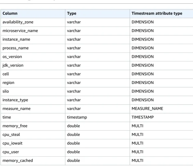
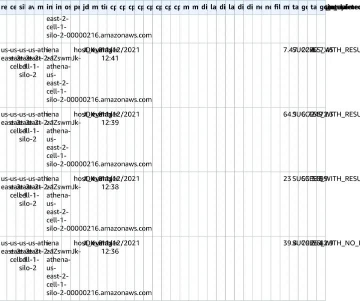
The table below shows an illustrative example for how Timestream stores data representing the CPU utilization, memory utilization, and network activity of EC2 instances, when the data is sent as a single-measure record. In this case, the dimensions are the region, availability zone, virtual private cloud, and instance IDs of the EC2 instances. The measures are the CPU utilization, memory utilization, and the incoming network data for the EC2 instances. The columns region, az, vpc, and instance_id contain the dimension values. The column time contains the timestamp for each record. The column measure_name contains the names of the measures represented by cpu-utilization, memory_utilization, and network_bytes_in. The columns measure_value::double contains measurements emitted as doubles (e.g. CPU utilization and memory utilization). The column measure_value::bigint contains measurements emitted as integers e.g. the incoming network data.

time region az vpc instance_id measure_namemeasure_value::doublemeasure_value::bigint 2019-12-04

19:00:00.000000000us-east-1 us-east-1d vpc-1a2b3c4di-1234567890abcdef0cpu_utilization35.0 null

(24)

time region az vpc instance_id measure_namemeasure_value::doublemeasure_value::bigint 2019-12-04

19:00:01.000000000us-east-1 us-east-1d vpc-1a2b3c4di-1234567890abcdef0cpu_utilization38.2 null 2019-12-04

19:00:02.000000000us-east-1 us-east-1d vpc-1a2b3c4di-1234567890abcdef0cpu_utilization45.3 null 2019-12-04

19:00:00.000000000us-east-1 us-east-1d vpc-1a2b3c4di-1234567890abcdef0memory_utilization54.9 null 2019-12-04

19:00:00.000000000us-east-1 us-east-1d vpc-1a2b3c4di-1234567890abcdef0network_bytes34,400 null 2019-12-04

19:00:01.000000000us-east-1 us-east-1d vpc-1a2b3c4di-1234567890abcdef0network_bytes1,500 null 2019-12-04

19:00:02.000000000us-east-1 us-east-1d vpc-1a2b3c4di-1234567890abcdef0network_bytes6,000 null

The table below shows an illustrative example for how Timestream stores data representing the CPU utilization, memory utilization, and network activity of EC2 instances, when the data is sent as a single- measure record.

time region az vpc instance_idmeasure_namecpu_utilizationmemory_utilizationnetwork_bytes 2019-12-04

19:00:00.000000000us-east-1 us-

east-1d vpc-1a2b3c4di-1234567890abcdef0metrics 35.0 54.9 34,400 2019-12-04

19:00:01.000000000us-east-1 us-

east-1d vpc-1a2b3c4di-1234567890abcdef0metrics 38.2 42.6 1,500 2019-12-04

19:00:02.000000000us-east-1 us-

east-1d vpc-1a2b3c4di-1234567890abcdef0metrics 45.3 33.3 6,600

Time series model

The time series model is a query time construct used for time series analytics. It represents data as an ordered sequence of (time, measure value) pairs. Timestream supports time series functions such as interpolation to enable you to ﬁll the gaps in your data. To use these functions, you must convert your data into the time series model using functions such as create_time_series. Refer to Query Language Reference (p. 273) for more details.

Using the earlier example of the EC2 instance, here is the same data expressed as a timeseries:

region az vpc instance_id cpu_utilization

us-east-1 us-east-1d vpc-1a2b3c4d i-1234567890abcdef0[{time:

2019-12-04

(25)

region az vpc instance_id cpu_utilization 19:00:00.000000000, value: 35}, {time:

2019-12-04

19:00:01.000000000, value: 38.2},

{time: 2019-12-04 19:00:02.000000000, value: 45.3}]

Scheduled Query

The scheduled query feature in Amazon Timestream is a fully managed, serverless, and scalable solution for calculating and storing aggregates, rollups, and other forms of preprocessed data typically used to power operational dashboards, business reports, ad-hoc analytics, and other applications. Scheduled queries make real-time analytics more performant and cost-eﬀective, so you can derive additional insights from your data, and can continue to make better business decisions.

With scheduled queries, you deﬁne the real-time analytics queries that compute aggregates, rollups, and other operations on their data—and Amazon Timestream periodically and automatically runs these queries and reliably writes the query results into a separate table. The data is typically calculated and updated into these tables within a few minutes.

You can then point your dashboards and reports to query the tables that contain aggregated data instead of querying the considerably larger source tables. This leads to performance and cost gains that can exceed orders of magnitude. This is because the tables containing aggregated data contain much less data than the source tables, so they oﬀer faster queries and cheaper data storage.

Additionally, tables with scheduled queries oﬀer all of the existing functionality of a Timestream table.

For example, you can query the tables using SQL. You can visualize the data stored in the tables using Grafana. You can also ingest data into the table using Amazon Kinesis, Amazon MSK, AWS IoT Core, and Telegraf. You can conﬁgure data retention policies on these tables for automatic data lifecycle management.

Because the data retention of the tables that contain aggregated data is fully decoupled from that of source tables, you can also choose to reduce the data retention of the source tables and keep the aggregate data for a much longer duration, at a fraction of the data storage cost. Scheduled queries make real-time analytics faster, cheaper, and therefore more accessible to many more customers, so they can monitor their applications and drive better data-driven business decisions.

Topics

• Scheduled Query Beneﬁts (p. 19)

• Scheduled Query Use Cases (p. 19)

• Example: Using real-time analytics to detect fraudulent payments and make better business decisions (p. 19)

• Scheduled Query Concepts (p. 20)

• Schedule Expressions for Scheduled Queries (p. 22)

• Data Model Mappings for Scheduled Queries (p. 24)

• Scheduled Query Notiﬁcation Messages (p. 37)

• Scheduled Query Error Reports (p. 40)

• Scheduled Query Patterns and Examples (p. 42)

(26)

Scheduled Query Beneﬁts

The following are the beneﬁts of scheduled queries:

• Operational ease – Scheduled queries are serverless and fully managed. All you need to do is deﬁne the required inputs, and Amazon Timestream will take care of the rest.

• Performance and cost – Because scheduled queries precompute the aggregates, rollups, or other real-time analytics operations for your data and store the results in a table, queries that access tables populated by scheduled queries contain less data than the source tables. Therefore, queries that are run on these tables are faster and cheaper. Tables populated by scheduled computations contain less data than their source tables, and therefore help reduce the storage cost. You can also retain this data for a longer duration in the memory store at a fraction of the cost of retaining the source data in the memory store.

• Interoperability – Tables populated by scheduled queries oﬀer all of the existing functionality of Timestream tables and can be used with all of the services and tools that work with Timestream. See Working with Other Services for details.

Scheduled Query Use Cases

You can use scheduled queries to power your business reports that summarize the end-user activity from your applications, so you can train machine learning models for personalization. You can also use scheduled queries to power alarms that detect anomalies, network intrusions, or fraudulent activity, so you can take immediate remedial actions.

Additionally, you can use scheduled queries for more eﬀective data governance. You can do this by granting source table access exclusively to the scheduled queries, and providing your developers access to only the tables populated by scheduled queries. This minimizes the impact of unintentional, long- running queries.

Example: Using real-time analytics to detect fraudulent payments and make better business decisions

Consider a payment system that processes transactions sent from multiple point-of-sale terminals distributed across major metropolitan cities in the United States. You want to use Amazon Timestream to store and analyze the transaction data, so you can detect fraudulent transactions and run real-time analytics queries. These queries can help you answer business questions such as identifying the busiest and least used point-of-sale terminals per hour, the busiest hour of the day for each city, and the city with most transactions per hour.

The system process ~100K transactions per minute. Each transaction stored in Amazon Timestream is 100 bytes. You’ve conﬁgured 10 queries that run every minute to detect various kinds of fraudulent payments. You’ve also created 25 queries that aggregate and slice/dice your data along various

dimensions to help answer your business questions. Each of these queries processes the last hour’s data.

You’ve created a dashboard to display the data generated by these queries. The dashboard contains 25 widgets, it is refreshed every hour, and it is typically accessed by 10 users at any given time. Finally, your memory store is conﬁgured with a 2-hour data retention period and the magnetic store is conﬁgured to have a 6-month data retention period.

In this case, you can choose to power your dashboards using real-time analytics queries that recompute the data every time the dashboard is accessed and refreshed, or power the dashboard using derived

(27)

tables. The query cost for dashboards based on real-time analytics queries will be $120.70 per month. In contrast, the cost of dashboarding queries powered by derived tables will be $12.27 per month (see this pricing sheet). In this case, using derived tables reduces the query cost by ~10 times.

Scheduled Query Concepts

Query string - This is the query whose result you are pre-computing and storing in another Timestream table. You can deﬁne a scheduled query using the full SQL surface area of Timestream, which provides you the ﬂexibility of writing queries with common table expressions, nested queries, window functions, or any kind of aggregate and scalar functions that are supported by Timestream query language.

Schedule expression - Allows you to specify when your scheduled query instances are run. You can specify the expressions using a cron expression (such as run at 8 AM UTC every day) or rate expression (such as run every 10 minutes).

Target conﬁguration - Allows you to specify how you map the result of a scheduled query into the destination table where the results of this scheduled query will be stored.

Notification configuration -Timestream automatically runs instances of a scheduled query based on your schedule expression. You receive a notification for every such query run on an SNS topic that you configure when you create a scheduled query. This notification specifies whether the instance was successfully run or encountered any errors. In addition, it provides information such as the bytes metered, data written to the target table, next invocation time, and so on.

The following is an example of this kind of notiﬁcation message.

{ "type":"AUTO_TRIGGER_SUCCESS",

"arn":"arn:aws:timestream:us-east-1:123456789012:scheduled-query/

PT1mPerMinutePerRegionMeasureCount-9376096f7309", "nextInvocationEpochSecond":1637302500, "scheduledQueryRunSummary":

{

"invocationEpochSecond":1637302440, "triggerTimeMillis":1637302445697, "runStatus":"AUTO_TRIGGER_SUCCESS", "executionStats":

{

"executionTimeInMillis":21669, "dataWrites":36864,

"bytesMetered":13547036820, "recordsIngested":1200, "queryResultRows":1200 }

} }

In this notiﬁcation message, bytesMetered is the bytes that the query scanned on the source table, and dataWrites is the bytes written to the target table.

Note

If you are consuming these notifications programmatically, be aware that new fields could be added to the notification message in the future.

Error report location - Scheduled queries asynchronously run and store data in the target table. If an instance encounters any errors (for example, invalid data which could not be stored), the records that encountered errors are written to an error report in the error report location you specify at creation of a scheduled query. You specify the S3 bucket and prefix for the location. Timestream appends the scheduled query name and invocation time to this prefix to help you identify the errors associated with a specific instance of a scheduled query.

(28)

Tagging - You can optionally specify tags that you can associate with a scheduled query. For more details, see Tagging Timestream Resources.

Example

In the following example, you compute a simple aggregate using a scheduled query:

SELECT region, bin(time, 1m) as minute,

SUM(CASE WHEN measure_name = 'metrics' THEN 20 ELSE 5 END) as numDataPoints FROM raw_data.devops

WHERE time BETWEEN @scheduled_runtime - 10m AND @scheduled_runtime + 1m GROUP BY bin(time, 1m), region

@scheduled_runtime parameter - In this example, you will notice the query accepting a special named parameter @scheduled_runtime. This is a special parameter (of type Timestamp) that the service sets when invoking a speciﬁc instance of a scheduled query so that you can deterministically control the time range for which a speciﬁc instance of a scheduled query analyzes the data in the source table. You can use @scheduled_runtime in your query in any location where a Timestamp type is expected.

Consider an example where you set a schedule expression: cron(0/5 * * * ? *) where the scheduled query will run at minute 0, 5, 10, 15, 20, 25, 30, 35, 40, 45, 50, 55 of every hour. For the instance that is triggered at 2021-12-01 00:05:00, the @scheduled_runtime parameter is initialized to this value, such that the instance at this time operates on data in the range 2021-11-30 23:55:00 to 2021-12-01 00:06:00.

Instances with overlapping time ranges - As you will see in this example, two subsequent instances of a scheduled query can overlap in their time ranges. This is something you can control based on your requirements, the time predicates you specify, and the schedule expression. In this case, this overlap allows these computations to update the aggregates based on any data whose arrival was slightly delayed, up to 10 minutes in this example. The query run triggered at 2021-12-01 00:00:00 will cover the time range 2021-11-30 23:50:00 to 2021-12-30 00:01:00 and the query run triggered at 2021-12-01 00:05:00 will cover the range 2021-11-30 23:55:00 to 2021-12-01 00:06:00.

To ensure correctness and to make sure that the aggregates stored in the target table match the aggregates computed from the source table, Timestream ensures that the computation at 2021-12-01 00:05:00 will be performed only after the computation at 2021-12-01 00:00:00 has completed, and the results of the latter computations can update any previously materialized aggregate using if a newer value is generated. Internally, Timestream uses record versions where records generated by latter instances of a scheduled query will be assigned a higher version number. Therefore, the aggregates computed by the invocation at 2021-12-01 00:05:00 can update the aggregates computed by the invocation at 2021-12-01 00:00:00, assuming newer data is available on the source table.

Automatic triggers vs. manual triggers - After a scheduled query is created, Timestream will

automatically run the instances based on the speciﬁed schedule. Such automated triggers are managed entirely by the service.

However, there might be scenarios where you might want to manually trigger some instances of a scheduled query. Examples include if a speciﬁc instance failed in a query run, if there was late-arriving data or updates in the source table after the automated schedule run, or if you want to update the target table for time ranges that are not covered by automated query runs (for example, for time ranges before creation of a scheduled query).

You can use the ExecuteScheduledQuery API to manually initiate a speciﬁc instance of a scheduled query by passing the InvocationTime parameter, which is a value used for the @scheduled_runtime parameter.

The following are a few important considerations when using the ExecuteScheduledQuery API:

• If you are triggering multiple of these invocations, you need to make sure that these invocations do not generate results in overlapping time ranges. If you cannot ensure non-overlapping time ranges,

Amazon Timestream

Amazon Timestream

Developer Guide

Amazon Timestream: Developer Guide

Copyright © Amazon Web Services, Inc. and/or its aﬃliates. All rights reserved.

Table of Contents

What Is Amazon Timestream?

Timestream Key Beneﬁts

Timestream Use Cases

Getting Started With Timestream

How It Works

Timestream Concepts

A summary of Timestream Concepts

Architecture

Write Architecture

Storage Architecture

Query Architecture

Cellular Architecture

Note

Writes

Note

No upfront schema deﬁnition

Writing data (Inserts and Upserts)

Multi-measure records

Beneﬁts

Use cases

Example: Monitoring the performance and health of a video streaming application

Using single measure records

Using multi-measure records

Note

Writing data with a timestamp that exists in the past or in the future

Note

Note

Batching writes

Note

Eventual consistency for reads

Storage

Note

Query

Data Model

Note

Flat Model

Time series model

Scheduled Query

Scheduled Query Beneﬁts

Scheduled Query Use Cases

Example: Using real-time analytics to detect fraudulent payments and make better business decisions

Scheduled Query Concepts

Note