利用改良式小波轉換技術進行結構損傷評估

(1)

國立臺灣大學工學院土木工程學系碩士論文

Department of Civil Engineering College of Engineering National Taiwan University

Master Thesis

利用改良式小波轉換技術進行結構損傷評估 Application of Modified Wavelet Transform for

Damage Assessment of Civil Structure Using Vibration Measurements

薛汶 Wen Hsueh

指導教授：羅俊雄博士 Advisor: Chin-Hsiung Loh, Ph.D.

中華民國 106 年 6 月

June, 2017

(2)

口試委員會審定書

(3)

ACKNOWLEDGEMENT

本研究得以順利完成，首先要感謝恩師羅俊雄教授的指導與教誨。在研究過

程中，老師悉心指導並給予無數的建議、方向與諮詢，提供豐富的學習資源與環境，

在學期間更提供機會讓學生到國外參與研討會，和學者交流開拓國際視野，非常感謝恩師的付出與提攜。此外還要感謝呂良正教授、周中哲教授、張國鎮教授在口試期間的指導與建議，使本研究更加完整。

在研究期間，感謝學長黃謝恭、李宗憲、葉乃睿、學姊黃昱婷、學妹郭采蓉、

吳瑀心、學弟余以諾、李全富在實驗以及研究上提供協助與解惑。此外感謝同學林佳樺、凃雅瀞以及陳俊達，在這兩年中的鼓勵與扶持，互相幫助並解決學習與研究上的問題。另外感謝同學夏瑄、葉柔伶以及其他同學的陪伴，讓我的研究所生活增添許多歡笑。有了各位學長姐、同學、學弟妹的互相幫助與學習，讓我的研究生活趨於豐富完整。

最後萬分感謝一直陪伴著我的家人，父親薛公堯、母親邱真鳳以及弟弟薛皓

尹，您們的支持與體貼，讓我能無後顧之憂地專心學習與研究。謹以此文獻給您們，

願您們與我一同分享這份喜悅與榮耀。

(4)

ABSTRACT (IN CHINESE)

對於時變系統的結構健康監測，小波轉換已被廣泛應用於取得局部時間的特徵相關訊息。本研究提出改良式小波轉換技術搭配可調式複數莫萊小波進行結構損傷評估，同時也提供較佳的時頻圖表示及簡化訊號重組。基於小波轉換得到的小波係數，本文介紹七種損傷指標包含：(1) Marginal spectrum, (2) Central frequency, (3) Pseudo-instantaneous frequency, (4) Unwrapped phase, (5) Novelty index, (6) Correlation, (7) Normalized component energy。本研究使用兩組振動台試驗的試體

（雙塔鋼構架、三層樓鋼構架）以及兩棟實際結構（花蓮明禮國小、台中中興大學）

來進行驗證，由分析結果顯示，本文提出之方法能夠取得結構物全域與局部特徵並有效進行結構損傷評估。

關鍵詞: 結構健康監測、小波轉換、可調式複數莫萊小波、結構損傷評估、結構損傷部位識別

(5)

ABSTRACT (IN ENGLISH)

For detecting transient signals and time-varying systems, wavelet transform has been used as a signal pattern recognition method for feature extraction. In this study, dynamic response data of structure using modified complex Morlet wavelet with variable central frequency (MCMW+VCF) is used to establish a time-frequency representation of measurement for modal parameter estimation and system damage identification. The proposed wavelet transform (WT) provides a better representation in generating scalogram than using general wavelet transform, besides, the proposed WT can simplify the choice of wavelet parameters and signal reconstruction. Based on the wavelet coefficients, several damage assessment algorithms will be described, which include: (1) Marginal spectrum, (2) Central frequency, (3) Pseudo-instantaneous frequency, (4) Unwrapped phase, (5) Novelty index, (6) Correlation, and (7) Normalized component energy. Seismic response data collected from two lab experiments, a twin tower steel

structure and two 3-story steel structures, under a series of both white noise as well as earthquake excitation back to back will be used to demonstrate the proposed algorithms.

Also, two field experiments, seismic response of Mingli elementary school and NCHU Civil & Environmental Engineering Building, will be used for the verification, too. The performance of the proposed algorithms is capable for damage detection and localization.

(6)

Keywords: structural health monitoring, wavelet transform, modified complex Morlet wavelet, damage detection, damage localization

(7)

LIST OF TABLES

Table 3-1 Test protocol of twin-tower steel structure ... 62 Table 3-2 Test protocol of two three-story steel frames ... 62

(11)

LIST OF FIGURES

Figure 1-1 The flowchart of the pattern-level feature extraction technique... 63 Figure 2-1 The shapes of Shannon, Complex Morlet, and Mexican Hat wavelets in

time and frequency domain (All the wavelets have the same analysis frequency of 5 Hz) ... 64

Figure 2-2 The shape of complex Morlet wavelet in different parameters a and b (fixed ₀ 1 Hz) with 1 (top) and  2 (bottom) in time and frequency domain ... 64

Figure 2-3 The shape of complex Morlet wavelet in different central frequency (fixed a1) with 1 (top) and 1 (bottom) in time and frequency domain

... 65 Figure 2-4 The relationship between



, time duration (top left) and frequency

bandwidth (top right). The definition of time duration is 0.95



(t) (bottom left) and frequency bandwidth is ^max



^⁽^⁾



^/ ² (bottom right) ... 65 Figure 2-5 Signal padding operation for using  2 ... 66 Figure 2-6 The wave form of the simulated nonlinear time functions ... 66 Figure 2-7 Plot time-frequency analysis of the test signal s(t); (a) using general

CWT, (b) using MCMW+VCF, (c) the instantaneous frequency using Hilbert

(12)

Figure 2-8 One-story two-bay reinforced concrete frame ... 67

Figure 2-9 Dimension of RC frame ... 68

Figure 2-10 The scalogram of RC frame (a) using general CWT, (b) using MCMW+VCF with  1, (c) using MCMW+VCF with  2 ... 68

Figure 2-11 The acceleration of RC frame (top) and the ridge calculated from different wavelet transform (bottom) ... 69

Figure 2-12 Discrete wavelet transform tree ... 69

Figure 2-13 Wavelet packet transform tree ... 70

Figure 2-14 Wavelet packet transform tree (in Paley order) ... 70

Figure 3-1 The twin-tower steel structure ... 71

Figure 3-2 Damage scenario-1, 2, and 3 of the twin-tower steel structure ... 71

Figure 3-3 Sensor instrumentations for the twin-tower steel structure ... 72

Figure 3-4 The maximum interstory drift ratio for twin-tower steel structure ... 72

Figure 3-5 The central frequencies for twin-tower steel structure (w.r.t. frequency band: 0~6 Hz) ... 73

Figure 3-7 The Novelty index for twin-tower steel structure (w.r.t. frequency band: 0~6 Hz) ... 74

(13)

Figure 3-8 The Novelty index for twin-tower steel structure (w.r.t. frequency band:

0~10 Hz) ... 74

Figure 3-9 The correlation for twin-tower steel structure (w.r.t. frequency band: 0~6 Hz) ... 75

Figure 3-10 The correlation for twin-tower steel structure (w.r.t. frequency band: 0~10 Hz) ... 75

Figure 3-11 The normalized CE for twin-tower steel structure (w.r.t. frequency band: 0~6 Hz) ... 76

Figure 3-12 The normalized CE for twin-tower steel structure (w.r.t. frequency band: 0~10 Hz) ... 76

Figure 3-13 Two three-story steel frames ... 77

Figure 3-14 Components of each floor for two three-story steel frames ... 77

Figure 3-15 Configuration of the two three-story steel frames ... 78

Figure 3-16 Sensor instrumentations for the two three-story steel frames... 78

Figure 3-17 Hysteresis loop of specimen-1 ... 79

Figure 3-18 Hysteresis loop of specimen-2 ... 80

Figure 3-19 The maximum interstory drift ratio for two three-story steel frames ... 81

Figure 3-20 The maximum story drift for specimen-2 ... 81

(14)

Figure 3-21 The central frequency for two three-story steel frames (w.r.t. x-dir.

frequency band: 0~5 Hz, torsional dir. frequency band 25~40 Hz ) ... 81

Figure 3-22 The Novelty index for two three-story steel frames (w.r.t. x-dir. frequency band: 0~5 Hz, torsional dir. frequency band 25~40 Hz) ... 82

Figure 3-23 The correlation for two three-story steel frames (w.r.t. x-dir. frequency band: 0~5 Hz, torsional dir. frequency band 25~40 Hz) ... 82

Figure 3-24 The normalized CE for two three-story steel frames (w.r.t. x-dir. frequency band: 0~5 Hz, torsional dir. frequency band 25~40 Hz) ... 83

Figure 4-1 The analysis frequency band of complex Morlet wavelet ... 84

Figure 4-2 The hysteresis loop for RC frame ... 84

Figure 4-3 The pseudo-IF using different extraction methods ... 85

Figure 4-4 The time history of the simulated nonlinear SDOF system... 86

Figure 4-5 The hysteresis loop of the simulated nonlinear SDOF system ... 86

Figure 4-6 The pseudo-IF of the simulated nonlinear SDOF system ... 86

(15)

Figure 4-9 The pseudo-IF for damage scenario-1 with sensing node A-5 (top) and sensing node B-4 (bottom) ... 88 Figure 4-10 The pseudo-IF for damage scenario-2 with sensing node A-5 (top) and

sensing node B-4 (bottom) ... 89 Figure 4-11 The pseudo-IF for damage scenario-3 with sensing node A-5 (top) and

sensing node B-4 (bottom) ... 90 Figure 4-12 The unwrapped phase for damage scenario-1 (w.r.t. frequency band:

0~10 Hz) ... 91 Figure 4-13 The unwrapped phase for damage scenario-2 (w.r.t. frequency band:

0~10 Hz) ... 91 Figure 4-14 The unwrapped phase for damage scenario-3 (w.r.t. frequency band:

0~10 Hz) ... 92 Figure 4-15 The central frequency for two three-story steel frames (w.r.t. x-dir.

frequency band: 0~5 Hz, torsional dir. frequency band 0~50 Hz ) ... 92 Figure 4-16 The pseudo-IF for two three-story steel frames in x-dir. with specimen-1

(top) and specimen-2 (bottom) (w.r.t. x-dir. frequency band: 0~5 Hz) ... 93 Figure 4-17 The pseudo-IF for two three-story steel frames in torsion direction with

specimen-1 (top) and specimen-2 (bottom) (w.r.t. torsional dir. frequency band:

25~40 Hz) ... 93

(16)

Figure 4-18 The unwrapped phase for two three-story steel frames in x-dir. with specimen-1 (1^st and 3^rd row) and specimen-2 (2^nd and 4^th row) (w.r.t. x-dir.

frequency band: 0~5 Hz) ... 94 Figure 4-19 The unwrapped phase for two three-story steel frames in torsional dir.

with specimen-1 (1^st and 3^rd row) and specimen-2 (2^nd and 4^th row) (w.r.t. torsional dir. frequency band: 0~50 Hz) ... 95 Figure 5-1 Sensor instrumentations for the Mingli Elementary School ... 96 Figure 5-2 The peak acceleration (PA) of every recorded earthquake event ... 96 Figure 5-3 The recorded accelerations of basement in y-dir. (top) and x-dir. (bottom)

... 97 Figure 5-4 The central frequency for the Mingli Elementary School (w.r.t. y-dir.

frequency band: 1.5~5 Hz, x-dir. frequency band 1~4 Hz ) ... 98 Figure 5-5 The unwrapped phase for the Mingli Elementary School (w.r.t. y-dir.

frequency band: 1.5~5 Hz, x-dir. frequency band 1~4 Hz ) ... 98 Figure 5-6 The pseudo-IF for EV04 (1996/09/05) (w.r.t. frequency band: 0.5~6 Hz

for both directions) ... 99 Figure 5-7 The pseudo-IF for EV05 (1999/09/20) using relative acceleration (w.r.t.

frequency band: 0.5~6 Hz for both directions) ... 100

(17)

Figure 5-8 The pseudo-IF for EV06 (1999/09/20) (w.r.t. frequency band: 0.5~6 Hz for both directions) ... 101 Figure 5-9 The pseudo-IF for EV05 (2006/12/26) (w.r.t. frequency band: 0.5~6 Hz

for both directions) ... 102 Figure 5-10 The pseudo-IF for EV05 (2010/10/02) (w.r.t. frequency band: 0.5~6 Hz

for both directions) ... 103 Figure 5-11 Sensor instrumentations for the NCHU Civil & Environmental

Engineering Building ... 104 Figure 5-12 The peak ground acceleration (PGA) of every recorded earthquake event

... 104 Figure 5-13 The recorded accelerations of 1F in x-dir. (top) and y-dir. (bottom) .... 105 Figure 5-14 The central frequency for the NCHU Civil & Environmental Engineering Building (w.r.t. frequency band: 1~4 Hz for both direction) ... 106 Figure 5-15 The unwrapped phase for the NCHU Civil & Environmental Engineering Building (w.r.t. frequency band: 1~4 Hz for both direction) ... 106 Figure 5-16 The pseudo-IF for EV09 (1996/03/05) (w.r.t. frequency band: 0.5~6 Hz

for both directions) ... 107 Figure 5-17 The pseudo-IF for EV13 (1999/09/20) using relative acceleration (w.r.t.

frequency band: 0.5~6 Hz for both directions) ... 108

(18)

Figure 5-18 The pseudo-IF for EV27 (1999/09/24) (w.r.t. frequency band: 0.5~6 Hz for both directions) ... 109 Figure 5-19 The pseudo-IF for EV59 (2006/03/09) (w.r.t. frequency band: 0.5~6 Hz

for both directions) ... 110 Figure 5-20 The pseudo-IF for EV94 (2009/11/05) (w.r.t. frequency band: 0.5~6 Hz

for both directions) ... 111

(19)

Chapter 1. Introduction

1.1 Background

Structural system identification and damage detection have received more and more attention in the field of civil engineering. Through monitoring data on structures, a quantity of information can be obtained. A well-known classification for damage identification methods can be defined as four levels: (Level-1) Determination or detection that damage is present in the structure; (Level-2) Determination of the geometric location of the damage; (Level-3) Quantification of the severity of the damage; (Level-4) Prediction of the remaining service life of the structure. One of the efficient and accurate damage detection techniques applicate to all types of structural systems is the vibration- based damage detection (VBDD). The vibration characteristics of a structure can be considered to be a global response signature that can be used as the basis for assessing its condition because they contain embedded information about the structure’s inherent properties. Changes in the structural condition will be reflected in the vibration signature, which make it possible to identify the presence of damage by tracking changes to that signature. Fourier-based analysis has been used as a means of translating vibration signals from time domain into the frequency domain to detect the vibration signatures. But the Fourier transform is not able to present the time dependency of signals and it cannot

(20)

measured from the vibration of structures. Wavelet transform can be viewed as an extension of the traditional Fourier transform with the adjustable window location and size, which has recently emerged as a promising tool for structural health monitoring (SHM) and damage detection due to its inherent properties. Its widespread use is also due to its availability of fast and accurate computational algorithms for signal transformation and reconstruction.

Early work using wavelet analysis for SHM has been carried out from several perspectives. From a system identification perspective, Basu and Gupta (1997) applied wavelet analysis to obtain the spectral moments and peak structural responses of multi- degree-of-freedom (MDOF) systems subjected to nonstationary seismic excitations.

Staszewski (1997) used time-scale decomposition to identify the damping in MDOF systems. Todorovska (2001) used the continuous wavelet transform to estimate the instantaneous frequency of signals. Kijewski and Kareem (2003) used wavelet analysis for system identification. Lardies and Ta (2005) used a wavelet-based approach to estimate the instantaneous frequency, damping, and envelope of the system. Li and Liang (2012) proposed a generalized synchrosqueezing transform to enhance the signal time- frequency representation. Tarinejad and Damadipour (2014) used modified Morlet wavelet to estimate damping. Klepka and Uhl (2014) identified the modal parameters of non-stationary systems with the recursive method based on the wavelet adaptive filter.

(21)

Chen et al (2014) detected the sudden stiffness reduction in acceleration time history using discrete wavelet transform. Guo and Kareem (2015) utilized the transformed singular value decomposition in tandem to automate the identification of analysis regions in the time-frequency domain. Subsequently, Laplace wavelet filtering is adopted to extract impulse-type signals from the WT coefficients to estimate the damping from transient nonstationary data. From a signal processing perspective, Robertson et al (2003) used Holder exponent based on the wavelet transform to detect the presence of damage and determine when the damage occurred. Goggins et al (2007) divided wavelet coefficients into several frequency bands and the degree of correlation between coefficients of ground and response acceleration was evaluated and allowed yielding and buckling events to be detected. Nair and Kiremidjian (2009) use a wavelet energy based approach to detect the damage. Noh et al (2011) use wavelet-based damage-sensitive features (DSFs) extracted from structural responses recorded during earthquakes to diagnose structural damage. Lee et al (2014) proposed a continuous relative wavelet entropy-based reference-free damage detection algorithm for truss bridge structures and showed that it was sensitive to slight damage extent for the tested damage type (i.e.

loosening of bolts). Balafas and Kiremidjian (2015) developed and validated a novel earthquake damage estimation scheme based on the continuous wavelet transform of input and output acceleration measurements. Amezquita-Sanchez and Adeli (2015) used

(22)

the synchrosqueezed wavelet transform fractality model to detect, locate, and quantify the damage in smart high-rise building structures.

1.2 Research objectives

The objective of this study is to utilize the pattern-level feature extraction technique through the continuous wavelet transform (CWT) with the proposed modified complex Morlet wavelet with variable central frequency (MCMW+VCF) to decompose the vibration responses into wavelet coefficient distribution as a joint function of time and frequency. The flowchart of the pattern-level feature extraction technique is shown in Figure 1-1. Different from centralized feature extraction, pattern-level feature extraction technique uses response measurement from individual sensing node. Then based on the extracted features, several damage assessment techniques can be implemented using the pattern-level fusion techniques.

The organization of this study is briefly described as follows:

Chapter 1: A brief description of the research background and the literature survey on the existing identification techniques based on the wavelet transform is presented. Then a general introduce to the objective and scope of this research.

Chapter 2: Introduce the wavelet analysis including the continuous wavelet transform (CWT), discrete wavelet transform (DWT), and wavelet packet transform (WPT). More

(23)

details of the CWT will also be described. By making use of the CWT, vibration features of structure can be extracted and then applied to structural damage identification.

Chapter 3: In this chapter, 5 damage assessment algorithms based on the extracted features will be described, which include: (1) Marginal spectrum, (2) Central frequency, (3) Novelty index, (4) Correlation and (5) Normalized component energy. Response measurement from two lab experiments will be firstly introduced then used to validate the proposed methods.

Chapter 4: Based on the features extracted from earthquake response data, 4 algorithms can be used to identify the damage, which include: (1) Marginal spectrum, (2) Central frequency, (3) Pseudo-instantaneous frequency, and (4) Unwrapped phase. Also, the same two experiments from shaking table tests that have been introduced in chapter 3 will be utilized to verify the algorithms.

Chapter. 5: The earthquake response data collected from two building structures under earthquake excitation will be used to verify the proposed methods.

Chapter. 6: Discussion and conclusion for the use of the proposed methods will be given.

The future work of this topic will also be indicated.

(24)

Chapter 2. Signal Analysis Methodology

2.1 The Continuous Wavelet Transform

2.1.1 The Continuous Wavelet Transform

The continuous wavelet transform (CWT) is a linear transformation, represents the signal x(t) as a sum of dilated and time-shifted wavelets in the form:

* (b,a)

[ ]( , ) ( ) ( ) W x b a_ ^ x t t dt







^(2.1.1)

* *

(b,a)

( ) 1 t b

t a a

   ^ ^ ^

  (2.1.2)

in which (t)L²() is called the mother wavelet and * represents a complex conjugate.

The mother wavelet (t) is dilated by various a, which are the scale parameters defining

the analysis window stretching, and shifted parameters b, which localize the wavelet

function in the time domain. The factor a^¹^/² is used to ensure energy preservation.

These basic functions are convoluted with x(t) to compute the wavelet coefficients

) , ](

[x b a

W_ . By this approach, one can examine the signal at different time window and frequency band by controlling the wavelet’s translation and dilatation. The higher the value of wavelet coefficient, the more similar the wavelet basis is to the original signal.

One can observe the variation of wavelet coefficients from the scalogram, which take the modulus of wavelet coefficients and show in time-scale plane with different color patterns

(25)

wavelet will provide different result of CWT. Therefore, the selection of an appropriate mother wavelet is an important issue which will be discussed in section 2.1.2.

The mother wavelet ψ(t) should satisfied the following admissibility condition to ensure existence of the inverse wavelet transform such as

2

0

ˆ ( )

W_   d

 







  ^(2.1.3)

where ˆ() is the Fourier transform of (t). The existence of the integral in equation

(2.1.3) requires that

ˆ (0) 0

  , i.e., ^( )t dt 0





 ^(2.1.4)

The signal x(t) can be reconstructed by an inverse wavelet transform of

) , ](

[x b a

W_ as defined by

( , ) 2

0

1 1

( ) [ ]( , ) _{b a} ( )

a b

x t W x b a t dbda

W_ ^ ^ ^  a

 



 

^(2.1.5)

2.1.2 The Mother Wavelets

There are countless mother wavelets used in practice for CWT. The wavelet analysis with real wavelet function like Mexican Hat unveils discontinuities or isolated peaks in the signal. For those who want to observe the phase variation, an analytical wavelet like the complex Morlet and Shannon can satisfy such requirement [6]. The scaling function

(26)

the infinite regularity permits an exact reconstruction.

Figure 2-1 shows the comparison between these three wavelets. All the wavelets have the same center frequency of 5 Hz. The result reveals that the Mexican Hat is simple zero phase wavelet, the complex Morlet wavelet has side lobes on both sides, and the Shannon wavelet is a leggy wavelet with a number of side lobes that die out on both sides.

One might suspect that the Morlet and Shannon wavelets will have somewhat lower temporal resolution due to their side lobes, in contrast to the Mexican Hat wavelet which should exhibit higher temporal resolution. But in Fourier Transform, Mexican Hat shows worse frequency resolution than other two’s and the complex Morlet wavelet shows best shape which matches the sharp peaks of signal in frequency domain. Therefore, for this data processing, the modified complex Morlet wavelet (MCMW) is used as the mother wavelet. The MCMW is defined as:

2 2

0 ( /2 )

( )t e eⁱ^^t ^t ^



 ^ (2.1.6)

which is essentially a complex exponential modulated by a Gaussian envelope and



is a measure of the spread in time.

The MCMW has Fourier transform

 0² ²

1

ˆ ( ) 2 e 2^{ } ^

    ^ ^ (2.1.7)

The scaled wavelet and its Fourier Transform are

2 2

0( ) ( ) /2

1 ⁱ^ ^{t b} ^{t b} ^

  ^ ^ ^

(27)

*

(b,a)( ) e ^{i b}^ ˆ(a )

 

 ^

 

(2.1.9)

For the Morlet wavelet, there is a unique relationship between the scale parameter a and Fourier frequency



, at which the wavelet is focus. The scale parameter a is inversely proportional to frequency



a 0

  (2.1.10)

Figure 2-2 shows the relationship between scale parameters a and analysis frequencies



for using central frequency ₀1Hz and also take into consider the



term for choosing  1 and 2. From the Figure, we can see the uncertainty principle of signal processing. As the scale parameter a1 (₀), it shows that an increase in

time resolution results in a decrease in frequency resolution, and vice versa. For the modified Morlet wavelet ( 2), it enhances the frequency resolution at the expense of time resolution.

2.1.3 Variable Central Frequency

Facing the uncertainty principle of signal processing, we change the general way of choosing different scales ( ₀ const. ) but to choose different central frequency

(aconst.) through the analysis frequencies.

0 1

a 

   (2.1.11)

Using this method, we can keep the resolution the same and change the coefficients

(28)

from time-scale analysis to time-frequency analysis:

*

0 (b, )

[ ]( , ) ( ) ( )

W x b_   ^ x t _ t dt



 



^(2.1.12)

Figure 2-3 shows the proposed variable central frequencies under  1 and 2.

Compare with Figure 2-2, the resolution remain the same through the analysis frequency for using proposed variable central frequency. And Figure 2-4 shows the relationship between



, time duration and frequency bandwidth under a1. We can see that if we choose larger



, the time duration gets longer and the frequency bandwidth becomes narrower which will provide smoother wavelet spectrum in time-axis and sharper spectrum in frequency-axis, and vice versa. It is optional for the user to choose proper



, for example, if we care more about the frequency domain than time domain like white noise data, we can choose larger sigma.

2.1.4 Edge effect melioration: Signal padding

The loss of considerable regions of a signal is the unfortunate consequence of edge effects. One possible solution to this problem is padding the beginning and end of the signal with real signal and leaving these values at the both sides to be corrupted by edge effect. Using this method, the characteristics of the signal can be preserved [11]. Figure 2-5 shows an example of signal padding operation for using  2. From Figure 2-4,

(29)

reflect a portion of the signal (4.9 seconds) about its beginning and end to compute the wavelet coefficients.

2.1.5 The Parseval Equality and Computation of Wavelet Transform via FFT The Parseval equality for the inner product of two functions f and g is [22]

1 ˆ ˆ

( ) ( ) ( ) ( )

f t g t dt 2 f  g  d



 

 







^(2.1.13)

and it implies

 

* (b,a)

* ( , )

*

1 *

[ ]( , ) ( ) ( ) 1 ˆ( )ˆ ( ) 2

1 ˆ( )ˆ ( ) 2

ˆ( )ˆ ( )

b a

i b

W x b a x t t dt

f d

f a e d

FT f a







   



   



  



















(2.1.14)

Then general W_[x](b,a) can be computed efficiently using Fourier Transform by

first computing fˆ() and ˆ^*(a), and then computing the inverse transform of the

product fˆ(



)



ˆ^*(a



). The proposed W_[x](b,) can also be computed via the same approach.

2.1.6 Example 1 (Simulation)

(30)

variable central frequencies (MCMW+VCF), a nonlinear time function is generated and shown in Figure 2-6 [21]:

1 2 3

( ) ( ) ( ) ( )

s t s t s t s t (2.1.15)

where

1

/15 1.2

2

1.3 3

( ) (1 0.2 cos(2 )) cos(2 (2 0.3cos( )))

( ) (1 0.3cos(2 )) cos(2 (2.4 0.5 0.3sin( ))) ( ) cos(2 (5.3 0.2 ))

t

s t t t t

s t t e t t t

s t t t





  

   

 

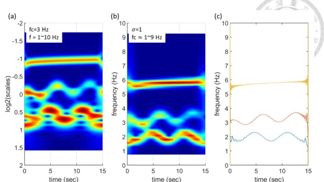
Application of the general CWT and the proposed MCMW+VCF to the nonlinear time function, Figure 2-7 shows the modulus of wavelet coefficients from these two methods in scalogram and the instantaneous frequency (IF) using Hilbert transform of the signals is also shown. We can see that using general CWT, the time resolutions are poor in lower frequencies, but using variable central frequencies, we can fix the resolution and provide better time-frequency representation.

2.1.7 Example 2 (Experiment)

The proposed method is also applied to the shaking table test of a SDOF RC frame [4] . The test specimen was a one-story two-bay frame (Figure 2-8) with overall height of 2 m and an approximate weight of 6454 kg, the dimension of the frame is shown in Figure 2-9. Take the average of the measurements from accelerometers A1, A4, and A7.

The results of the acceleration using general CWT and the proposed method using

(31)

different sigma ( 1,2) are shown in Figure 2-10. From these three scalograms, it’s

hard to compare the pros and cons of the two methods, it can only see that the bright regions under  2 are sharper and longer than other two. Using the scalogram to extract the ridge as instantaneous frequency (Figure 2-11), which will be describe in section 4.1.1, we can see that the general CWT provide poorer instantaneous frequency

in the initial small amplitude data because the energy preservation factor a^¹^/² provides larger weight for the analysis frequencies which are smaller than central frequency, it may also enlarge the frequency given by earthquake. And the difference between using sigma equals to 1 and 2 is that  2 provides more stable instantaneous frequency though the time of frequency shift is earlier than  1 due to its longer time duration.

2.2 The Discrete Wavelet Transform

The calculating wavelet coefficients at every possible scale will generate a lot of redundant data which is not desirable since more computations and more memory are necessary to process a signal with redundancy. Therefore, a discrete version of the wavelet is utilized by discretizing the dilation parameter a and the translation parameter b in signal processing. The procedure becomes much more efficient if dyadic values of a and b are used. That is,

2j

a ; b2^jk ,j kZ (2.2.1)

(32)

where Z is a set of integers, j is referred to as the level, and k is the shifting coefficient.

DWT can be viewed as the filtering process which decompose signal into two parts, the detail and approximate part. For the detail part, which using the high-pass filter (t),

is defined as:

/2 *

, 2 ^j ( ) (2 ^t )

cDj k ^ ^x t ^ t k dt







 ^(2.2.2)

For the approximate part derived from the low-pass filter (t):

/2 *

, 2 ^j ( ) (2 ^t )

cAj k ^ ^ x t  ^t k dt







 ^(2.2.3)

where (t) is the scaling function derived from the mother wavelet. Note that not every

wavelet function has scaling function and the algorithm is only available for orthogonal wavelet function which has scaling function and permits the fast algorithm. Due to the orthogonal property, a signal can be represented by its details and approximates. The detail and approximate at level j are defined as

, , ( )

j j k j k

k

D ^ cD  t







^(2.2.4)

, , ( )

j j k j k

k

A ^ cA  t







^(2.2.5)

It becomes obvious that

1

j j j

A_  A D (2.2.6)

( ) _j _j

x t  A 



j J_ D ^(2.2.7)

The DWT decomposition procedure can be shown as a DWT tree (Figure 2-12).

(33)

2.3 The Wavelet Packet Transform

Since the DWT only decompose the approximation part in lower frequency, the high frequency resolution remains the same. As a result, there might be the problem that the important information exists in the higher frequency. Therefore, to provide a better resolution, the wavelet packet transform (WPT) is developed to further decompose the detail components. The concept of WPT is shown as the WPT tree in Figure 2-13. The WPT is a function with three parameters:

/2

, ( ) 2 (2 )

i j i j

j k t t k







 , i0, 1, 2, ..., (2^j 1) (2.2.8)

where i, j and k refer to the modulation, scale and translation, respectively. The wavelet

i is obtain from the recursive relationships:

2ⁱ( ) 2 ( ) ⁱ(2 )

k

t h k t k

 ^ 







 ^(2.2.9)

2 1ⁱ ( ) 2 ( ) ⁱ(2 )

k

t g k t k

 ^ ^ 







 ^(2.2.10)

where h(k) and g(k) are quadrature mirror filters associated with the scaling function

and mother wavelet function. Note that ⁰ is the scaling function  and ¹ is the mother wavelet. Similar to DWT, the signal can be reconstructed by linear combination of decomposed components of WPT:

2 1

0

( ) ( )

j

i j i

x t x t







^(2.2.11)

The decomposed part of xⁱ_j(t) is represent by a linear combination of wavelet packet

(34)

, ,

( ) ( )

i i i

j j k j k

j

x t ^ c  t







^(2.2.12)

where the wavelet packet coefficient cⁱ_j_,_k can be obtained from:

, ( ) , ( )

i i

j k j k

c ^ x t t dt







^(2.2.13)

Providing that the wavelet packet functions are orthogonal

, ( ) , ( ) 0

m n

j k t j k t

 

 , if m n (2.2.14)

In WPT, the central frequency of wavelet component is not in ascending order resulted from the aliasing, instead, it’s a Paley order. Therefore, the ordering process need to be considered if the WPT technique is implemented. The Paley ordering process is illustrated in Figure 2-14.

2.4 Hilbert Transform

The Hilbert transform of a real-valued function x(t) extended over the range







 t is a real-valued function ~ tx( ) defined by [7]

 

^{( )}

( ) ( )

( )

x t H x t x u du

 t u





 



 ^(2.3.1)

Thus ~ tx( ) is the convolution integral of x(t) and 1/t, written as

( ) ( )*(1/ )

x t x t t (2.3.2)

The Hilbert transform is simply a 90 degrees rotation in the phase angle of the original

(35)

( ) ( ) ( )

z t x t ix t (2.3.3)

One can also write

( ) ( ) ⁱ ( )^t

z t A t e^ (2.3.4)

where A(t) is the Hilbert amplitude/ envelope signal of x(t) and (t) is the instantaneous phase signal of x(t).

2 2

( ) ( ) ( )

A t  x t x t (2.3.5)

1

0

( ) tan ( ) 2 ( )

t x t f t

  ^ ^x t ^ 

  (2.3.6)

The “instantaneous frequency” f₀ is given by

0

1 ( )

2

d t

f dt





 

   (2.3.7)

(36)

Chapter 3. Damage Assessment Algorithms -Ambient Vibration Data

In the damage assessment technology, the most commonly used indicator can be divided into two parts: physical features and damage indices. In this chapter, 5 algorithms will be introduced and applied to the ambient vibration data, which include: (1) Marginal spectrum, (2) Central frequency, (3) Novelty index, (4) Correlation, and (5) Normalized component energy. The first two are physical features and the others are damage indices.

These algorithms can provide the information about the healthy or damage state of the structure. Two experimental data will be utilized to verify these algorithms.

Because the wavelet parameter b has the meaning of time t , and 2 f ,

therefore, in the following discussion, we change the notation of wavelet coefficients from W_[x](b,) to W x t f_[ ]( , ).

3.1 Damage assessment algorithms

3.1.1 Marginal Spectrum

A traditional way to investigate signals includes the spectral analysis through Fourier transform. The modal frequency of the structure will induce a peak in the Fourier spectrum, but sometimes it’s hard to find the modal frequency because of the high

(37)

near that position. The marginal spectrum of the MCMW+VCF provides smoother and lower-resolution spectrum which can be defined as:

( ) [ ]( , )

At

t

H f 



W x t f_ ^(3.1.1) Based on the marginal spectrum, the frequency band can be chosen to calculate the following damage assessment algorithms.

3.1.2 Central Frequency

An easy way to observe the global behavior of the structure under the excitation is central frequency, which is defined as:

2

( ) ( )

At j j

j

At j

j

H f f f 



H f



^(3.1.2)

where f_j is the selected frequency band from the marginal spectrum. The structural

stiffness degradation will cause the change of system dominant frequency. Hence, the identification of central frequency can provide the dominant frequency of the structure and also a rough assessment of damage severity by only analyzing the output signal.

3.1.3 Novelty Index (reference-based index)

The shapes of the wavelet coeﬃcients time-frequency plots can be compared by

visual inspection, or alternatively, Novelty index. Novelty detection aims to establish

(38)

simply whether or not a new pattern is significantly different from a previous pattern.

Consider the white noise response measurement, based on the MCMW+VCF, the Novelty index (NIn) is defined as:

( , ) ( , )

( , )

i ref

A j A j

t j

i ref

A j

t j

H t f H t f

NIn H t f







, i: for test case i (3.1.3)

( , ) [ ]( , )

H t fA W x t f_ (3.1.4)

where H_A(t,f) is the modulus of wavelet coefficients, H_A^ref(t,f) is refer to as the undamaged reference data, and f_j is the selected frequency band from the marginal

spectrum. Novelty index can compare not only the frequency shift but also energy change due to the damage.

3.1.4 Correlation (reference-based index)

Another comparison of scalograms of the wavelet coefficients is by correlating both sets of data for the selected frequency band [13] . The correlation coefficient is defined as

  

 

²

 

²

( , ) ( , ) ( , ) ( , )

i i ref ref

A j A j A j A j

t j

i

i i ref ref

A j A j A j A j

t j t j

H t f H t f H t f H t f

Corr

H t f H t f H t f H t f

 



 



 

^(3.1.5)

where the bar denotes the mean of the wavelet coefficients and f_j is the selected

frequency band from the marginal spectrum.

(39)

3.1.5 Normalized Component Energy

For the small ambient vibration and white noise, the response signal can be normalized by input signal. It is shown that the energy of the wavelet coefficients are functions of the physical parameters of the system and loading functions. Therefore, the normalized component energy (normalized CE) can be used as a damage assessment index, which is defined as:

( , ) ( , )

i

E j

t j

input

E j

t j

H t f Normalized CE

H t f





, i: for i^th floor (3.1.6)

where H_E( , )t f W x t f_[ ]( , )² is the component energy and f_j is the selected

frequency band from the marginal spectrum.

3.2 Application to Twin-tower Structure with Weak Bracing System

3.2.1 Set-up of monitoring system

The first model used for the experimental verification is the twin-tower structure. A steel structure with two towers (tower-A: 5 story and tower-B: 4 story) connected at basement as well as the 1^st floor (Figure 3-1) was constructed and tested on the shaking table in National Center of Research on Earthquake Engineering (NCREE), Taipei, Taiwan. Each story with height of 1.17 m and 500 kg was added to each floor to simulate floor weight. The dimension of the plate was 1.1 m × 1.5 m × 0.02 m. The H-type

(40)

column with the dimension of 0.1 m × 0.03 m × 1.1 m was used for all floor. In EW- direction, the bracing system using L-shape angle steel with the dimension of 65 mm × 65 mm × 6 mm was designed with large bucking load to prevent transverse motion

during the test, and in NS-direction, the bracing system was designed with smaller buckling load as compare to the EW-direction. Two types of braces were used in NS- direction. The dimension of Brace1 was 19 mm × 1.2 mm to simulate the weak location and Brace2 with dimension of 21.3 mm × 2 mm was used as normal condition. Three different damage scenarios were created. Damage scenrario-1 was to create buckling in the 1^st floor of tower-A, damage scenario-2 was to create buckling in the 2^nd floor of tower-A, and damage scenario-3 was to create bucking in the 2^nd floor of tower-B. The buckling of three cases was setup by installing weak bracing members (Brace1) in that floor. The configuration of the structure is shown in Figure 3-2. There were in total 22 accelerometers, 22 LVDTs instrumented in this experiment. For tower-A, 12 accelerometers and 12 LVDTs in x-direction for all floors and tower-B had the same instrumentation as tower-A with 10 accelerometers and 10 LVDTs in x-direction for all floors. The distribution of accelerometer and the LVDT is shown in Figure 3-3. The sampling rate of all the sensor devices is 200 Hz. The spectrum compatible acceleration record (from Chi-Chi earthquake station TCU071) was used as the desired base excitation of the shaking table. The base excitation was arranged back to back with different input

(41)

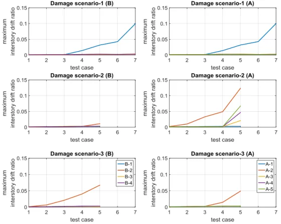
intensity level and applied in x-direction only (North direction). In between the earthquake excitation, white noise excitation (with peak acceleration of 50 gal) was also applied to serve as the reference state of the structure before and after each earthquake excitation. The test protocol for damage scenario-1, 2, and 3 are shown in Table 3-1. Take average of the LVDT records ( (Disp_{X Right}_ Disp_{X Left}_ ) / 2) collected from earthquake for

each floor to calculate the maximum interstory drift ratio (IDR) (Figure 3-4). For damage scenario-1, the 1^st floor of two towers both show the increasing IDR with test cases because of the connection in that floor. For damage scenario-2, the increasing IDR in 2^nd floor of tower-A matches the setup of weak location. And there is also the slight changes of IDR in tower-B. For damage scenario-3, though the setup of weak location is in the 2^nd floor of tower-B, there is apparent interstory drift ratio happened in the 2^nd floor of tower- A after test case 4. This implies that there is also damage occurred in that floor.

3.2.2 Pre-processing procedure

Data collected from white noise will be used in this chapter. Take average of the absolute acceleration in x-direction ((Acc_X__Right Acc_X__Left)/2 ) for each floor as the

motion in longitudinal direction.

White Noise Response Data

Applying the proposed MCMW+VCF to the white noise acceleration response. Here

(42)

we focus more on the frequency domain than time domain, therefore, we choose  2 to enhance the frequency resolution. The scalogram of wavelet coefficients and the marginal spectrum are shown in Appendix I. For damage scenario-1, we can see that the dominant change of frequency happened in the 1^st mode for both tower-A and tower-B.

There’s almost no frequency shift from WN1 to WN4 and apparent frequency shift shows in WN5, after that, WN6 and WN7 show the frequency shift, too. For damage scenario- 2, the dominant frequency for 1^st floor of tower-A and all floor of tower-B occurs in 2^nd mode, but the dominant frequency of 2^nd to 5^th floor of tower-A is 1^st mode. For damage scenario-3, the dominant frequency changes from 2^nd mode to 1^st mode with the increase of test cases. Therefore, the frequency ranges of 0~6 Hz, which cover the 1^st mode, and 0~10 Hz, which cover the 1^st and 2^nd mode, will be used for the feature extraction.

3.2.3 The Results of Damage Assessment Central Frequency

The results of central frequency are plotted in Figure 3-5 (w.r.t. frequency band: 0~6 Hz) and Figure 3-6 (w.r.t. frequency band: 0~10 Hz). For damage scenario-1, the central frequencies of two frequency bands both show the decrease with test cases and converge to the lowest floor, which indicate that the damage occurs in the lowest floor. For damage scenario-2, the central frequencies calculated from two bands both show the frequencies

(43)

from 2^nd to 5^th floor of tower-A decrease and converge to the 2^nd floor, which indicate that the damage happens in the 2^nd floor. On the other hand, the small increase of frequencies in 1^st floor of tower-A and all floor in tower-B may cause by the decrease of 2^nd mode, which can be seen in marginal spectrum (Appendix I) and may also imply the damage occurrence. For damage scenario-3, the clearer change of central frequencies from 2^nd to 5^th floor of tower-B demonstrate that the damage locates in 2^nd floor of tower-B. From the observation, the frequencies decrease in WN4 w.r.t. frequency band: 0~6 Hz, but show earlier drop in WN3 w.r.t. frequency band: 0~10 Hz. The reason resulting in this case is because the 2^nd mode in WN3 is close to the 1^st mode in WN1, therefore, the frequencies w.r.t. frequency band: 0~6 Hz do not show the changes in WN3, but reflect w.r.t.

frequency band: 0~10 Hz. The frequency changes in all floors of tower-A may imply the damage occurs in lower floor.

Novelty Index (NIn)

For each floor, using equation (3.1.3) to compare difference test cases with reference (WN1). The results of NIn w.r.t. two frequency bands are plotted in Figure 3-7 and Figure 3-8. For damage scenario-1, the 𝑁𝐼𝑛 increases with test cases, which means

the difference of scalogram between reference and test case is getting large, and indicates the damage extent is getting severer, too. Besides, the 𝑁𝐼𝑛 from different sensing node

are very similar. This indicates that each floor has similar response and explains the

(44)

possibility for damage locates in the 1^st floor. Similar approach also be applied to damage scenario-2 and 3. For damage scenario-2, the values of 𝑁𝐼𝑛 calculated from sensing node

A-2 to A-5 are very similar and larger than other sensing nodes, which demonstrates that the damage locates in the 2^nd floor of tower-A. And for damage scenario-3, the increase of NIn above 2^nd floor of tower-B are larger than others, which implies the severest damage occurs in 2^nd floor of tower-B. It has to mention that for damage scenario-2, the values of NIn in last test case does not show the apparent growth while the marginal spectrum shows the decrease of modal frequency. This brings out the disadvantage of NIn that the index cannot reflect the distance if the frequency shifts far away from the reference.

Correlation

For each floor, using equation (3.1.5) to compare difference test cases with reference (WN1). The results of correlation w.r.t. two frequency bands are plotted in Figure 3-9 and Figure 3-10. From the observation, this index can also can be used to detect and locate the damage, but same as the Novelty index, the correlation cannot reflect the distance if the frequency shifts far away from the reference.

Normalized Component Energy (Normalized CE)

The results of normalized CE w.r.t. two frequency bands are plotted in Figure 3-11 and Figure 3-12. For damage scenario-1, all the normalized CE converged to the lowest

(45)

floor, which indicates that the energy of all sensors are very similar and proves the damage location is in the 1^st floor. For damage scenario-2, the energy from sensing nodes A-2 to A-5 all converge together as the case number increases. On the other hand, the energy of other sensing nodes remain the same. This implies the damage location is at 2^nd floor of tower-A. For damage scenario-3, the normalized CE above 2^nd floor for two towers both show the changes while the 1^st floors remain stable. This implies the damage may occur in the 2^nd floor. But in this case, the trend is not consistent with the other two damage scenarios, therefore, it cannot show the degree of damage.

3.3 Application to Two Three-story steel frames

3.3.1 Set-up of monitoring system

The second model used for the experimental verification is the two three-story steel frames, specimen-1 and specimen-2 respectively (Figure 3-13). This experiment was also conducted in NCREE. The frames with an overall height of 3.51 m and an approximate total weight of each structure was 2.94 ton (include additional 0.5 ton on each floor). The dimension of the plate was 1.1 m × 1.5m × 0.02 m. Two types of rectangular columns were used in the steel frame test. The dimension of type-1 column was 0.15 m × 0.025 m × 1.1 m and in type-2 column, there was a reduction of thickness with dimension of 0.15 m × 0.015 m × 1.1 m to simulate a weaker column in comparison with type-1

(46)

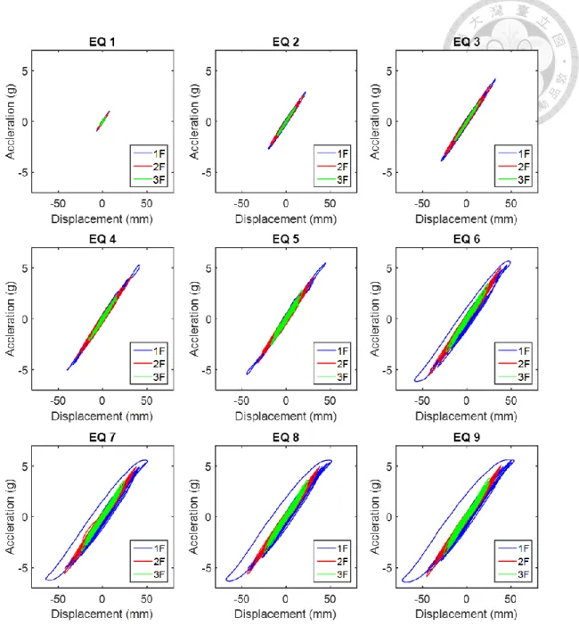
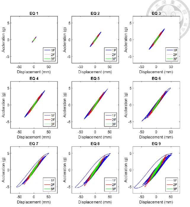
column. The components of the steel frames are shown in Figure 3-14, and the red column denotes the type-2 column. For specimen-1, type-1 columns were used for all floors while for specimen-2, one column in the 1^st floor at the north-west corner was replaced with type-2 column. Therefore, specimen-1 was a symmetric structure while specimen-2 was an anti-symmetric structure. The configuration of the steel frame test is shown in Figure 3-15. There were in total 18 accelerometers, 19 LVDTs instrumented in this experiment. For specimen-1, 6 accelerometers and 6 LVDTs in x-direction for all floors and specimen 2 had the same instrumentation as specimen 1 with additional 6 accelerometers and 6 LVDTs in y-direction for all floors. The distribution of accelerometer and the LVDT is shown in Figure 3-16. The sampling rate of all the sensor devices is 200 Hz. The spectrum compatible acceleration record (from Chi-Chi earthquake station TCU071) was used as the desired base excitation of the shaking table.

The base excitation was arranged back to back with different input intensity level and applied in x-direction only (North direction). In between the earthquake excitation, white noise excitation (with peak acceleration of 50 gal) was also applied to serve as the reference state of the structure before and after each earthquake excitation. The test protocol is shown in Table 3-2. With an increasing excitation level, the nonlinearity of the steel frame exhibits and the damage of the structure becomes more severe. The hysteresis loop in Figure 3-17 and Figure 3-18 both show that the nonlinearity become

利用改良式小波轉換技術進行結構損傷評估

國立臺灣大學工學院土木工程學系 碩士論文

Department of Civil Engineering College of Engineering National Taiwan University

Master Thesis

利用改良式小波轉換技術進行結構損傷評估 Application of Modified Wavelet Transform for

Damage Assessment of Civil Structure Using Vibration Measurements

薛 汶 Wen Hsueh

指導教授：羅俊雄 博士 Advisor: Chin-Hsiung Loh, Ph.D.

中華民國 106 年 6 月

June, 2017

口試委員會審定書

ACKNOWLEDGEMENT

ABSTRACT (IN CHINESE)

ABSTRACT (IN ENGLISH)

CONTENTS

LIST OF TABLES

LIST OF FIGURES









Chapter 1. Introduction

1.1 Background

1.2 Research objectives

Chapter 2. Signal Analysis Methodology

2.1 The Continuous Wavelet Transform







 





 

 





















 













2.2 The Discrete Wavelet Transform











2.3 The Wavelet Packet Transform















 

2.4 Hilbert Transform

 



Chapter 3. Damage Assessment Algorithms -Ambient Vibration Data

3.1 Damage assessment algorithms











  

 

 



國立臺灣大學工學院土木工程學系碩士論文

薛汶 Wen Hsueh

指導教授：羅俊雄博士 Advisor: Chin-Hsiung Loh, Ph.D.