國立臺灣大學工學院材料科學與工程學系暨研究所 碩士論文
Department of Materials Science and Engineering College of Engineering
National Taiwan University Master Thesis
運用 ReaxFF力場模型探討原子尺度下 鋰離子電池矽基負極鋰化動力學行為 Atomic-scale Modelling and Simulations of
the Lithiation Behavior of the Si Anode in Li-ion Batteries using Reactive Force Field (ReaxFF)
潘立毅 Li-Yi Pan
指導教授:郭錦龍 博士
Advisor: Chin-Lung Kuo, Ph.D.
誌謝
本論文的撰寫,首先要感謝兩年間指導教授郭錦龍教授的指導,
在思考問題上,常常能夠指出適當的方向,在學習解決問題的能力上 讓我獲益良多。也感謝翰昕、鈺杰、奕廷、嘉澤等前輩們指導一些模 擬條件上的修正,以及其他事務上的協助,使我能夠順利度過碩一的 階段。在 7/24(一)交論文的前夕,感謝有仁願意一同修改論文到晚上 4 點半左右,一些論文英文表達上的問題在當時獲得修正。感謝子敬 在這段時期的陪伴,稍微紓解了這段時間的壓力。在口試前一個禮拜 的 7/21(一)~7/23(三),也感謝張明揚、立揚與岡典犧牲休息時間的 幫忙,特別是三天間張明揚的全力支援。本人由衷感謝這段時間實驗 室同學們的幫助。希望同學們的研究,也能順利進行。
同時,也感謝這段時間內父母的支持,即使數據結果不理想,父 母也告訴我盡力而為,不要有太大壓力,讓我能專心研究,在艱難的 時刻,常常得到父母的鼓勵而能持續下去。也感謝口試委員趙聖德教 授、許文東教授與郭哲來教授在 7/28(五)口試時,對論文的不足點上 進行指正,使本論文能夠更臻完善。此外也感謝閒暇時刻朋友們聚會 時的加油打氣,以及提供研究上的一些意見。儘管本次論文內容與結 果不盡完美,也希望未來研究上能將之修正。最後謹在此對曾經獲得
Contents
1 Introduction 13
1.1 Research Backgrounds 13
1.1.1 The Li-ion battery and the anode materials 13
1.1.2 The charging process of silicon anode in Li-ion battery 14
1.1.3 The silicon nanowire anode in Li-ion battery 15
1.2 Motivation and Objectives 15
2 Literature Review 17
2.1 The experimental observations 17
2.2 Kinetic and Thermodynamic issues 17
2.3 Studies about silicon lithiation issues by ReaxFF. 20
3 Methodology 31
3.1 Molecular Dynamics 31
3.2 Reactive Force Field (ReaxFF) 33
4 ReaxFF Parameter Validation 37
4.1 Computational Details 37
4.1.1 Structural Properties 37
4.1.2 Thermodynamic Properties 38
4.3 Thermodynamical Properties 56
4.4 Mechanical Properties 62
4.5 Nudged Elastic Band calculation of lithium diffusion in crystalline silicon 64
4.6 Summary 65
5 Silicon lithiation rate comparison 67
5.1 Structure of silicon 67
5.2 Computational Details 69
5.3 Analysing Details 70
5.4 Results 72
5.4.1 Structural Observations in the Lithaition Mechanism 72
5.4.2 Lithiation Rates in Different Facets 77
5.4.3 Stress analysis in silicon slab 80
5.4.4 Lithiation Rates in Silicon Nanowires 80
5.4.5 Some Problems in this Study 86
5.4.6 Future Study 87
6 Conclusions 89
7 Appendix 91
7.1 Changes in order to make the energy volume curve smoother 91
7.2 The stress profile in the lithiation 92
8 References 99
Figures
1.1 The schematics of rechargeabble Li-ion battery (adapted from
Goodenough et. al.2) 13
2.1 The dumbbell-like shape formed in silicon nanowire lithaition
(adopted from Liu et al.5) 22
2.2 The crack found in silicon nanowire lithaition (adopted from Liu et al.5) 22 2.3 The anisotropic expansion in silicon nanowire lithaition (adopted
from Lee et al.6) 23
2.4 The phase boundary in silicon lithiation (adopted from Liu et al.7) 23 2.5 The ledge mechanism in silicon lithiation (adopted from Liu et al.7) 23 2.6 Chan et al.’s statement of the thermodynamic preference in silicon
lithiation. The figure in the left shows the formation energy and the lithiation voltage. The figure in the right compares the lithation voltage. The lithiation voltage is prefered in Si(110) facet and therefore the more energy is released when lithiating the Si(110)
facet than other facets. (adopted from Chan et al.8) 24 2.7 Jung et al.’s statement of the thermodynamic preference in silicon
lithiation. The first figure shows the surface energy 𝛾. The second figure shows the ratio of Li atoms to the interfacial Si(amorphous) atoms. The third figure shows the Li–Si(crystalline) bond to
2.9 The kinetic Monte Carlo simulation of sililcon nanowire anisotropic
expansion calculated by Cubuk et al.10 25
2.10 The shape of kinetic Monte Carlo simulation in sililcon nanowire
anisotropic expansion calculated by Cubuk et al.10 26 2.11 The anisotropic lithiation mechanism by Rohrer et al.11 27 2.12 The slab lithaition performed by Kim et al. (adopted from Kim et al.12) 27 2.13 The ReaxFF nanowire lithaition in NVT 300 K. The anisotropy is
reproduced. (adopted from Jung et al.13) 28
2.14 The stress analysis in ReaxFF nanowire lithaition (adopted from Jung
et al.13) 28
2.15 The stress effect on the lithiation rate. (adopted from Ostadhossein et
al.14) 29
2.16 The compressive stress effect on the Li diffusion energy barrier
(adopted from Ding et al.15) 29
2.17 The vacancy effect on the lithiation rate (adopted from Kim et al.16) 30 3.1 The bond order function and the bond breaking behavior in ReaxFF 35 4.1 The illustration of the nudge elastic band method 43
4.2 The energy volume curve of c-Si 44
4.3 The energy volume curve of c-LiSi 44
4.4 The energy volume curve of c-Li12Si7 45
4.5 The energy volume curve of c-Li13Si4 45
4.6 The energy volume curve of c-Li15Si4 46
4.7 The energy volume curve of c-Li Si 46
4.9 The radial distribution function of Li–Li in a-Li32Si32 51 4.10 The radial distribution function of Li–Si in a-Li32Si32 51 4.11 The radial distribution function of Si–Si in a-Li32Si32 52 4.12 The radial distribution function of Li–Li in a-Li40Si24 52 4.13 The radial distribution function of Li–Si in a-Li40Si24 53 4.14 The radial distribution function of Si–Si in a-Li40Si24 53 4.15 The radial distribution function of Li–Li in a-Li50Si14 54 4.16 The radial distribution function of Li–Si in a-Li50Si14 54 4.17 The radial distribution function of Si–Si in a-Li50Si14 55 4.18 The pressure vs. volume curve comparison between ReaxFF and
Stillinger Weber in NVT 1200 K 55
4.19 The formation energy of c-LixSi 57
4.20 The mixing energy of c-LixSi 58
4.21 The formation energy of a-LixSi 58
4.22 The mixing energy of a-LixSi 59
4.23 The formation energy comparison of amorphous and crystalline Li–Si alloys 59 4.24 The mixing energy comparison of amorphous and crystalline Li–Si alloys 60
4.25 The volume expansion of a-LixSi 60
4.26 The melting point of Si 61
4.27 The melting point of Li 61
4.28 The energy barrier of Li diffusion in Si by ReaxFF in this study 64
5.3 The silicon and the lithium in all Tdsite. The silicon is in ivory color while the lithium is in pink. The lithium should not be connected since there are no covalent bonding between them. The Li–Li connection is only used to show the duality of the silicon and lithium
structure and the diffusion path of lithium in silicon. 68
5.4 The silicon with lithium slab used in this study 71
5.5 The lithiation in NVT 1000 K at 100 ps. 72
5.6 The RDF 800 K result 73
5.7 The RDF 1000 K result 74
5.8 The RDF 1200 K result 75
5.9 Kim’s et al. result of RDF in lithiation 76
5.10 The temperature dependence on the lithiation rate difference 78 5.11 The anisotropy is reproduced in the Si[110] nanowire. The silicon is
removed for clarity. The subfigure above shows the orignial settings while the subfigure below shows the nanowire after 72 ps. The
anisotropy is reproduced. 82
5.12 The anisotropy is also reproduced in the Si[100] nanowire. The silicon is removed for clarity. The subfigure above shows the original settings while the subfigure below shows the nanowire after NVT
160 ps. The anisotropy is reproduced. 83
5.13 The Si[110] nanowire in NPT 600 K. The structure hardly lithiates.
Si(110) has much larger phase boundary than other facets. 84
5.14 The anisotropy is also reproduced in the Si[100] nanowire. The silicon is removed for clarity. The subfigure above shows the original settings while the subfigure below shows the nanowire after NPT 300 K 74.2 ps. with z-direction fixed and adding compressive stress on
the 𝑥- and 𝑦-direction 85
7.1 The Si(100) maximum principal stress in NVT 800 K 93 7.2 The Si(110) maximum principal stress in NVT 800 K 93 7.3 The Si(111) maximum principal stress in NVT 800 K 94 7.4 The Si(112) maximum principal stress in NVT 800 K 94 7.5 The Si(100) maximum principal stress in NVT 1000K 95 7.6 The Si(110) maximum principal stress in NVT 1000K 95 7.7 The Si(111) maximum principal stress in NVT 1000K 96 7.8 The Si(112) maximum principal stress in NVT 1000K 96 7.9 The Si(100) maximum principal stress in NVT 1200K 97 7.10 The Si(110) maximum principal stress in NVT 1200K 97 7.11 The Si(111) maximum principal stress in NVT 1200K 98 7.12 The Si(112) maximum principal stress in NVT 1200K 98
Tables
2.1 The thickness of phase boundary and the lithiation velocity in each facets 20
4.1 The lattice constant of Li, Si and their alloys 48
4.2 The comparison of ReaxFF and Bader charge of Li in crystalline
Li–Si alloy (unit: e) 48
4.3 The comparison of ReaxFF and Bader charge of Li in amorphous
Li–Si alloy (unit: e) 49
4.4 The cutoff radius used in the coordination number determiniation 49 4.5 The coordination number of a-Li32Si32, a-Li40Si24and a-Li50Si14 50 4.6 The comparison of ReaxFF formation energy with Fan et al.’s data
and DFT data. (unt: kcal/mol) 56
4.7 The calculated stiffness tensor in silicon (unit: GPa) 62
4.8 The mechanical properties of c-Si (unit: GPa) 62
4.9 The mechanical properties of c-Li (unit: GPa) 63
4.10 The mechanical properties of c-LiSi (unit: GPa) 63
4.11 The mechanical properties of c-Li15Si4(unit: GPa) 63 5.1 Dimensions of the Si slab used in this simulation (20 Å vacuum layer
for surface structure simulation is excluded from the table) 69 5.2 Dimensions of the Li slab used in this simulation 69
5.3 The NVT lithation rate comparison (unit: Å/ns) 77
Abstract
Li-ion battery is important in energy storages application such as portable electronic de- vices or electric cars. In most of Li-ion batteries, the anode material is graphite. Some researchers have found that the Si anode has a specific capacity approximately 10-fold larger than graphite. Therefore, it is deemed as a promising anode material. However, it suffers from the fracture problem in charging, due to the anisotropic expansion. This will strongly hinders the performance and cyclability. In this thesis, we will study the lithiation mechanism of Si anode by Reactive Force Field (ReaxFF) molecular dynamics simulations. We have performed the silicon slab lithiation to observe the lithiation be- havior at different temperature, and we have reproduced some anisotropy in this case. On the other hand, we have also performed the nanowire lithiation to show the anisotropic expansion. Our results show that the lithiation behavior is mainly kinetic controlled rather than thermodynamic controlled. We suggest that it is the lithium insertion preference in the Si(110) facets that leads to the anisotropic expansion. We have also analyzed the stress developed in the silicon. There are still some problems in the simulations, such as the energy discontinuity and the anomalous lattice constant at high temperature in ReaxFF, and some of which are still under investigation. In the future study, we will perform the simulation at lower temperature and higher lithium concentration to fully reproduce the anisotropic lithiation behavior.
摘要
鋰電池為現今重要的能量儲存裝置,並且被廣泛運用於可攜帶電 子裝置、電動車等。目前大部分的商業用鋰電池負極材料使用的是石 墨。然而,研究人員發現以矽作為負極材料的鋰電池擁有石墨電極約 10 倍的單位(重量)電容量。因此被視為鋰電池負極材料的明日之星。
然而,矽負極的充電會造成矽的破裂,這主要是由矽負極的不等向膨 脹所引起。矽的破裂將嚴重影響鋰電池的表現與可循環使用性。本研 究將探討矽負極材料的鋰化機制,我們將使用 Reactive Force Field (ReaxFF)的分子動力學模擬探討此問題。我們計算並觀察矽的平板在 不同溫度下的鋰化行為,我們部分複製了在實驗中觀察到的不等向膨 脹。除此之外,我們也使用了奈米線鋰化並觀察到非等向膨脹。由計 算結果我們認為是動力學主導了不等向膨脹的問題。我們認為鋰在 Si(110)方向的高擴散速度是此不等向膨脹的主因。我們分析了在鋰化 過程中矽所產生的應力。本次模擬仍有一些問題,包括了 ReaxFF 在 能量上的斷點、以及在高溫下不尋常的晶格常數等問題,其中有部分 我們仍舊需要找出癥結點。在未來研究中,我們將會在低溫且高鋰濃 度下進行鋰化,以完整複製實驗結果觀察到的非等向膨脹。
CHAPTER 1 Introduction
1.1 Research Backgrounds
1.1.1 The Li-ion battery and the anode materials
Rechargeable Li-ion battery has been introduced in 19801and it has been commercialized in 1991. It has been widely used in portable devices or electric cars. As in a normal battery system, it has 3 major parts: anode, cathode and electrolytes.
Figure 1.1 The schematics of rechargeabble Li-ion battery (adapted from Goodenough et. al.2)
In Li-ion battery, the anode (negative electrode) material undergoes an oxidation reac- tion (loss electron) while the cathode (positive electrode) material undergoes an reduction reaction (gain electron) during discharging process. The charging process is its counter- reaction and the oxidation-reduction relation is reversed.
• Cathode
LiCoO2→ Li1−𝑥CoO𝑥+ 𝑥𝑒−+ 𝑥Li+
• Anode (Graphite) : intercalating reaction
C + 𝑥𝑒−+ 𝑥Li+ → Li𝑥C
for 0 ≤ 𝑥 ≤ 1/6
However, it was found that the silicon anode can have a better capacity.3Its reaction can be written as below
• Anode (Silicon) : alloying reaction
Si + 𝑥𝑒−+ 𝑥Li+ → Li𝑥Si
for 0 ≤ 𝑥 ≤ 3.75
One can calculate that the theoretical energy capacity of graphite anode is 372.24 mAh/g while it is 3579.80 mAh/g for silicon anode.3 Therefore, silicon is a promising anode material in future Li-ion battery and has been widely researched. In this study, we will focus on the silicon anode and its properties during charging.
1.1.2 The charging process of silicon anode in Li-ion battery
The charging process of Li intercalation in graphite anode has been illustrated in figure 1.1. The Li ion was inserted into the interspacing of graphite. The silicon anode does not store lithium by intercalating but alloying mechanism. The main difference is that the Si–
Si bond will be broken during the charging process, while this is not the case for graphite anode. This process is called the lithiation of silicon anode.
silicon battery suffers from serious volume expansion problem as 400% expansion during lithiation. This will make the silicon anode vulnerable to break and pulverize into smaller particle. This leads to the capacity fading in Li-ion battery.
1.1.3 The silicon nanowire anode in Li-ion battery
In order to solve the problem of volume expansion. Chan et al. have proposed the silicon nanowire anode4in Li-ion battery. They have achieved better cyclability than the thin- film or nanoparticle counterparts. However, some cracks are still found in the nanowire.
This will be explained in the literature review part. The anisotropic expansion in silicon nanowire, particularly in Si[110] direction, makes the Li–Si alloy surface under large ten- sile stress and cracks the nanowire.
1.2 Motivation and Objectives
In this study, we want to characterize the reason why the silicon nanowire undergoes the anisotropic lithiation. We want to find out if it is the thermodynamic or kinetic issues that caused the anisotropy. We will use the Reactive Force Field (ReaxFF) in our study. We will compare the lithiation rate of different facets in silicon. The temperature contribution to the lithiation rate will be discussed. Besides, the anisotropic expansion of silicon nanowire will be illustrated.
CHAPTER 2 Literature Review
2.1 The experimental observations
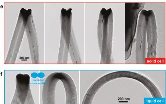
The anisotropic expansion in silicon nanowire lithiation has been observed experimentally by many groups. Liu et al. have observed dumbbell-shaped cross section (figure 2.1) in silicon nanowire lithiation.5 Besides, the crack is also observed in the center of the nanowire, shown in figure 2.2.
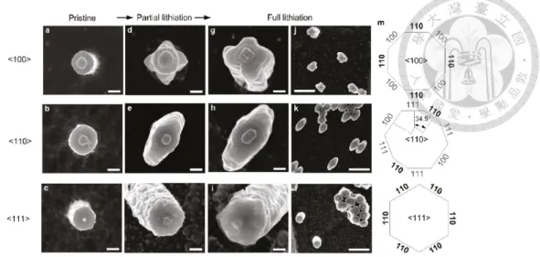
Besides, Lee et al. have performed the lithiation of silicon nanopillars6with orientation of ⟨100⟩, ⟨110⟩ and ⟨111⟩ and observed that the Si(110) has much higher lithiation rate than Si(100) and Si(111). The result is shown in figure 2.3. All of their observations shows a higher lithiation rate in Si(110) than other facets.
In addition, Liu et al. have conducted an in situ imaging7of the lithiation of silicon nanowire. In their study, they have reported a comparable lithiation rate between Si(110) facet and Si(112) facet. They have also observed the lithiation front (figure 2.4) during an in-situ TEM obsrvation. The Si(112) facet have a clear reaction front while Si(110) ’s is blur. It was shown in the supporting information of the paper. A ledge mechanism is proposed to explain the lithiation in Si(112) facet. These results are shown in figure 2.5.
2.2 Kinetic and Thermodynamic issues
It has been a long debate for the lithiation anisotropy is a thermodynamic or kinetic driven process. In the following section, some of the points will be reviewed.
favorable for lithiation in Si(110) facets than any other one. They performed a lithium in- sertion algorithm in the tetrahedral site of silicon and check for its changes. After that, they calculated the formation energy and the lithiation voltage (figure 2.6) of the Li–Si alloy formed in Si(100), Si(110) and Si(111) and concluded that Si(110) has a higher voltage and therefore higher energy preference in lithiation.
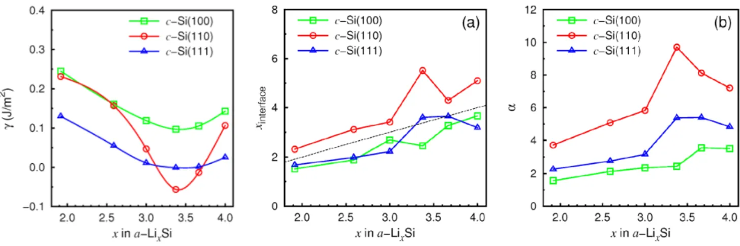
Jung et al. have also conducted an ab initio calculation9for the a-LixSi/c-Si surface and calculated the interface energy for Si(100), Si(110) and Si(111). The surface energy is defined as
𝛾 = (𝐸𝑡𝑜𝑡− 𝐸𝑎−𝐿𝑖𝑥𝑆𝑖− 𝐸𝑐−𝑆𝑖)/(2𝐴) (2.1)
The surface energy and surface Li/Si concentration results are shown in figure 2.7. They have arrived at 2 results:
1. The Si(110) has the lowest surface energy among all facets at 𝑥 = 3.4 in a-LixSi.
2. The Li surface concentration is the highest in Si(110) facets.
Therefore the energy stability of the lithiation in Si(110) is confirmed. Besides, the high lithium concentration will also enhance the lithiation rate.
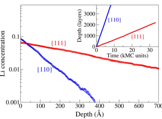
Kinetic issues about the lithiation anisotropy
Cubuk et al. have conducted another ab initio calculation10to check the orientation depen- dence on the energy barrier (figure 2.8). After obtaining the energy barrier, they performed the kinetic Monte Carlo simulation to calculate the shape evolution. It is concluded that the Li will tend to concentrate in the surface layer in Si(110) facet, while Li will go into the deeper layer in Si(111) facet by comparing the energy barrier difference. The concentra-
Rohrer et al. have also conducted an ab initio calculation on the lithiation process11. They have calculated the energy preference (shown as below, the higher the more energet- ically preferred) for each lithiation step in different facets.
• Li adsorption on c-Si: (100) < (111) < (110).
• Li (clean) penetration into c-Si: (100) < (110) < (111).
• Li (full-Li covered) penetration into c-Si: (111) ≑ (100) < (110).
• Surface energy preference of a-Li2Si/c-Si: (110) < (100) < (111).
• Energy barrier preference of Li (full-Li) diffuse into c-Si: isotropic.
• Energy barrier preference of Li (a-Li2Si) diffuse into c-Si: isotropic.
• Nucleus formation (a-LixSi formation in Si) energy preference: (100) < (111) < (110).
In addition to the different concentration of Li–Si alloy (a-Li2Si/c-Si) are used from Jung et al.’s paper(a-Li3.57Si/c-Si). The paper have mentioned a complete different view- point about the surface energy preference with Jung’s statement9. They argued that the facet with the lowest surface energy will be the most stable facet and will be harder to move. Therefore, when focusing on the nucleus formation preference term, the Si(110) has the highest nucleus formation energy. Thus the Si(110) is preferred than other facets.
The illustration is shown in figure 2.11.
Therefore, we want to clarify whether the thermodynamic issue, which is the energy preference of the product and the reactant, or kinetic issues, which is the energy barrier between the product and the reactant, are more important in the lithiation process. Un-
2.3 Studies about silicon lithiation issues by ReaxFF.
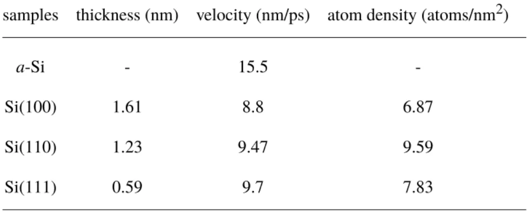
Kim et al. have performed the molecular dynamic (MD) simulations12 to check if the lithiation anisotropy can be reproduced. They used the reactive force field (ReaxFF) and Si(100), Si(110) and Si(111) slab with plenty of Li above it for lithiation. The simulation is carried out in 1200 K and the results are shown in figure 2.12. They have observed the phase boundary in the simulation and comfirmed its structure as c-LiSi (not exactly, however). The calculated velocity is also shown in table 2.1. They multiplied the layer density and the lithiation rate and concluded that Si(110) has the highest lithiation rate.
This weighted lithiation rate for Si(100), Si(110) and Si(111) are 1.0, 1.52 and 1.27 re- spectively in their study (normalized by Si(100)).
samples thickness (nm) velocity (nm/ps) atom density (atoms/nm2)
a-Si - 15.5 -
Si(100) 1.61 8.8 6.87
Si(110) 1.23 9.47 9.59
Si(111) 0.59 9.7 7.83
Table 2.1 The thickness of phase boundary and the lithiation velocity in each facets
Jung et al. have performed another ReaxFF-MD simulation for the lithiation of silicon nanowire.13They used 2 nanowire with Si(100) and Si(110) facets and Li surrounded for lithiation. The lithiation is carried out in NVT 300 K and the anisotropy is reproduced (figure 2.13). The anisotropy that they reproduced is more obvious than Kim et al.’s. They
the stress is somehow very large and I suspected that the volume is not divided in the raw data of LAMMPS, which output stress in the unit of stress⋅volume.
Ostadhossein et al. have also performed an ReaxFF-MD simulation14 to check the stress dependence of the lithiation rate. They used the Si(112) facet (the same as Liu et al.
mentioned previously7) and performed the lithiation in NVT 600 K. The ledge mechanism of the Si peeling off as in Liu et al.’s study is again observed. Besides, They have also observed that a compressive stress is developed near the phase boundary and concluded that a compressive stress of 4.5 GPa can stop the lithiation. They have performed another NPT simulation with compressive stress of 1 to 3 GPa on Si(110) facet to show that a compressive stress can slow down the lithiation rate. (figure 2.15)
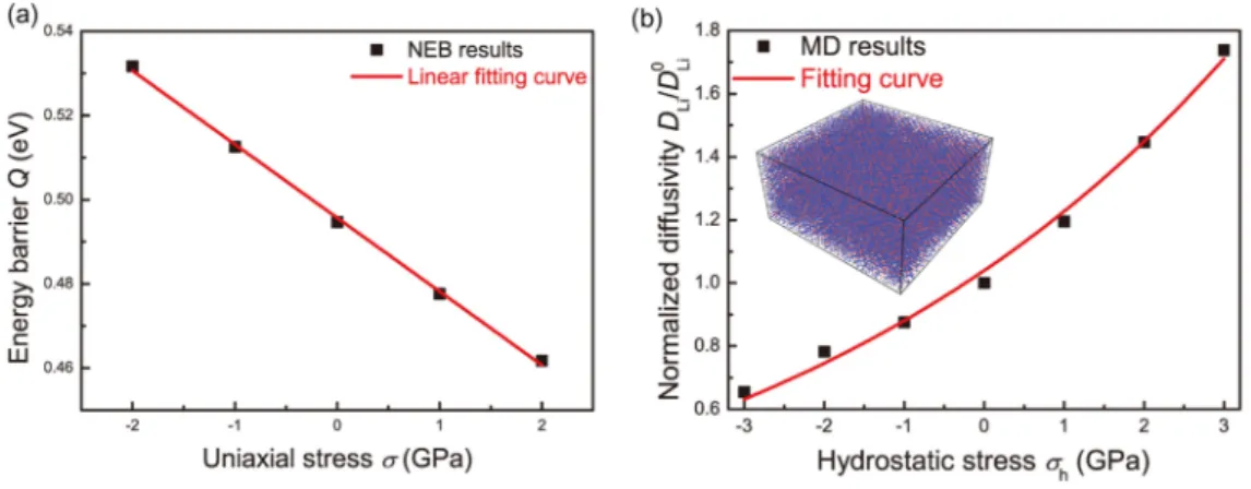
Just recently, Ding et al. have performed an ReaxFF simulation15to check the stress dependence of the Li diffusion energy barrier. They used nudged elastic band (NEB) to show that the diffusion energy barrier can be harder to overcome due to the compressive stress (figure 2.16).
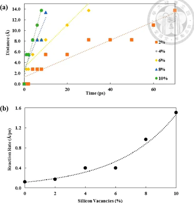
While in terms of vacancy influence. Kim et al. have also performed ReaxFF-MD simulation16 in NVT 900–1500 K to check the vacancy influence in the lithiation rate.
They have concluded that the introducing of Si vacancy accelerates the lithiation rate (fig- ure 2.17). It therefore suggested that the breaking of Si–Si bond is the rate-limiting factor in the lithiation of silicon anode.
Summarizing the studies above, we have known that
• These studies are done in various temperature ranging from 300 K to 1200 K. The
than 1200 K as in Kim et al.’s12.
• Compressive stress can have a suppressing effect on the lithiation rate in 600 K as mentioned by Ostadhossein et al.14. It was further explained by calculating the Li dif- fusion barrier as in Ding et al.’s paper.15
• A different lithiation mechanism is observed in 900–1500 K by Kim et al.16 which states that the Si–Si bond breaking is the rate-limiting factor.
Therefore, we want to characterize the effect of temperature in this study.
Figure 2.1 The dumbbell-like shape formed in silicon nanowire lithaition (adopted from Liu et al.5)
Figure 2.3 The anisotropic expansion in silicon nanowire lithaition (adopted from Lee et al.6)
Figure 2.4 The phase boundary in silicon lithiation (adopted from Liu et al.7)
Figure 2.5 The ledge mechanism in silicon lithiation (adopted from Liu et al.7)
Figure 2.6 Chan et al.’s statement of the thermodynamic preference in silicon lithiation. The figure in the left shows the formation energy and the lithiation voltage. The figure in the right compares the
lithation voltage. The lithiation voltage is prefered in Si(110) facet and therefore the more energy is released when lithiating the Si(110) facet than other facets. (adopted from Chan et al.8)
Figure 2.7 Jung et al.’s statement of the thermodynamic preference in silicon lithiation.
The first figure shows the surface energy𝛾. The second figure shows the ratio of Li atoms to the interfacial Si(amorphous) atoms. The third figure shows the Li–Si(crystalline) bond to interfacial Si(amorphous)–Si(crystalline) bond ratio. The interface energy is prefered in Si(110) and therefore Si(110) is much stable than other facets. (adopted from Jung et al.9)
Figure 2.8 The energy barrier calculated by Cubuk et al.10
Figure 2.9 The kinetic Monte Carlo simulation of sililcon nanowire anisotropic expansion calculated by Cubuk et al.10
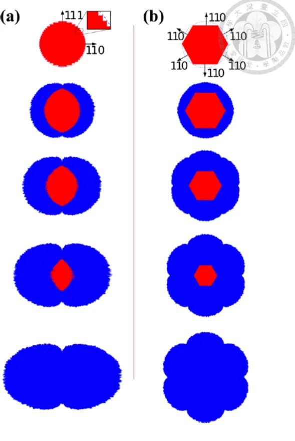
Figure 2.10 The shape of kinetic Monte Carlo simulation in sililcon nanowire anisotropic expansion calculated by Cubuk et al.10
Figure 2.11 The anisotropic lithiation mechanism by Rohrer et al.11
Figure 2.13 The ReaxFF nanowire lithaition in NVT 300 K.
The anisotropy is reproduced. (adopted from Jung et al.13)
Figure 2.15 The stress effect on the lithiation rate. (adopted from Ostadhossein et al.14)
Figure 2.16 The compressive stress effect on the Li diffusion energy barrier (adopted from Ding et al.15)
Figure 2.17 The vacancy effect on the lithiation rate (adopted from Kim et al.16)
CHAPTER 3 Methodology
3.1 Molecular Dynamics
In this study, we used the molecular dynamics with the Reactive Force Field (ReaxFF) implemented in LAMMPS to study the Si lithiation problem. The molecular dynamics simulation predicts the atomic movement by solving the Newton’s equation of motion by time integration. i.e. if there are 𝑛 atoms in the system and for each atom 𝑖, for all 1 ≦ 𝑖 ≦ 𝑛, we have.
𝐅𝑖(𝑡) = 𝑚𝑖d2𝐱𝑖(𝑡)
d𝑡2 (3.1)
while
𝐅𝑖(𝑡) = The force vector imposed on atom 𝑖 at time 𝑡 𝑚𝑖 = The atomic mass of atom 𝑖
𝐱𝑖(𝑡) = The position vector of atom 𝑖 at time 𝑡
Therefore, if the initial position 𝐱𝑖(𝑡) and the force 𝐅𝑖(𝑡) is given, the moving trajectory can be calculated. The classical molecular dynamics, which utilizes a force field, is adopted in this study. This means that the potential energy surface
𝑉 = 𝑉 (𝐱1, 𝐱2, ..., 𝐱𝑛) (3.2)
In order to solve the equation of motion (3.1), the initial velocity and position must be given. This is done by giving a random velocity with their absolute value in Gaussian distribution for each atom.
While the acceleration (solved by force) ¨𝐱, velocity ˙𝐱 and position 𝐱 of each atom (from now on, we dropped the 𝑖 in each atom for simplicity) are given, the problem remains is to solve the differential equation (3.1) by time integration. There are many ways to solve this initial value problem but the velocity Verlet algorithm17is the most widely adopted method. Given the position, velocity and acceleration of atoms in timestep 𝑛, it solves the position of atoms in the next time step 𝑛 + 1 by Taylor expansion:
𝐱𝑛+1= 𝐱𝑛+ ˙𝐱𝑛Δ𝑡 + ¨𝐱𝑛Δ𝑡2/2 (3.4)
The velocity Verlet algorithm utilized a velocity in time integration, which is not the case by original Verlet algorithm. It calculates the velocity of the next time step by
˙𝐱𝑛+1= ˙𝐱𝑛+ (¨𝐱𝑛+1+ ¨𝐱𝑛−1)Δ𝑡/2 (3.5)
Note that the acceleration can always be obtained by (3.3) if the potential surface and the position are given.
¨𝐱𝑛+1= −∇𝑖𝑉 (𝐱𝑛+1)/𝑚 (3.6)
By applying this iteration, the movement of all atoms in all time can be integrated.
In most cases, we want to control some envionmental variables such as pressure 𝑃, temperature 𝑇 in order to observe the dynamic behavior in different situations. This is called the ensembles. The simplest ensemble is NVE, which fixes the number of atoms,
ensemble fixed the volume and controls the temperature while the NPT ensemble controls the pressure and temperatures. They utilizes the Nosé Hoover thermostat and barostat for the control of temperature and pressure.
In summary, A classical molecular dynamics consists of the following elements:
• The molecular or crystal structure.
This is the structure of the simulation system of interest.
• The force field.
This is the energy function that depends on atomic position.
• The time integration algorithm.
This is the algorithm used to solve the Newton’s equation of motion.
• The statistic mechanical ensemble and simulation conditions.
The statistic mechanical ensemble like the microcanonical ensemble NVE, canonical ensemble NVT or isothermal-isobaric ensemble NPT, etc. can be imposed on the system to simulate the real world cae.
3.2 Reactive Force Field (ReaxFF)
The ReaxFF18is developed by van Duin et al. in 2001. It is first used for C/H system ini- tially. It is later modified by Chenoweth19et al. in 2008. Most of the simulation packages like LAMMPS20 and 21 or GULP22 and 23 utilize this functional form. The user-reaxc package in LAMMPS is a revision of the Aktulga et al.’s implementation21. The follow- ing parameter description can be found in the supporting information of Chenoweth et al.’s
𝐸system = 𝐸bond+ 𝐸lp + 𝐸over+ 𝐸under
+ 𝐸val+ 𝐸pen+ 𝐸coa+ 𝐸C2+ 𝐸triple+ 𝐸tors+ 𝐸conj + 𝐸H−bond+ 𝐸vdWaals+ 𝐸Coulomb
The ReaxFF utilizes the bond order to describe the energy surface of bond-breaking. The bond order (uncorrected) is described by the function below
𝐵𝑂𝑖𝑗′ = 𝐵𝑂′𝑖𝑗𝜎+ 𝐵𝑂′𝑖𝑗𝜋+ 𝐵𝑂′𝑖𝑗𝜋𝜋
= exp [𝑝𝑏𝑜,1(𝑟𝑖𝑗 𝑟𝜎0)
𝑝𝑏𝑜,2
] + exp [𝑝𝑏𝑜,3(𝑟𝑖𝑗 𝑟𝜎0)
𝑝𝑏𝑜,4
] + exp [𝑝𝑏𝑜,5(𝑟𝑖𝑗 𝑟𝜎0)
𝑝𝑏𝑜,6
]
The energy of each term is a function of the bond order. e.g. for the first term 𝐸𝑏𝑜𝑛𝑑 we have
𝐸𝑏𝑜𝑛𝑑 = −𝐷𝜎𝑒𝐵𝑂𝑖𝑗𝜎exp[𝑝𝑏𝑒,1(1 − (𝐵𝑂𝜎𝑖𝑗)𝑝𝑏𝑒,2)] − 𝐷𝑒𝜋𝐵𝑂𝑖𝑗𝜋− 𝐷𝜋𝜋𝑒 𝐵𝑂𝜋𝜋𝑖𝑗 (3.7)
Figure 3.1 is the results of the Si–O reactive force field24published in 2003. It shows the energy–distance curve that the energy will be close to zero when the distance of Si–Si is larger enough. This is different from the traditional forcefield like harmonic oscillator ap- proximation, which will be the infinity when the distance goes to infinity. Since the atoms can be separated (bond-breaking) without being attracted. This will be able to describe the bond-breaking behavior, which is critical in our study since Si–Si bond must be broken in our study.
In addition to the bond-breaking behavior, ReaxFF is also able to describe the charge state in each atom. In the ReaxFF implemented by LAMMPS, it used the charge equili- bration scheme (Qeq)25to calculate the charge for each atom.
parameter is a enhanced parameter from Fan et al.27
The bond order function with respect to distance
CHAPTER 4 ReaxFF Parameter Validation
4.1 Computational Details
We have mentioned that the ReaxFF parameter that we used are taken from Ostadhossein et al.. In this part, we will validate the parameter by checking for the structural properties, charge, thermodynamical properties, mechanical properties and diffusion energy barrier of Li in Si by nudged elastic band method.
It is worth mention that when evaluating energy volume curve. Some break-points are found in the original parameter. Therefore, some changes are made in order to make the energy volume curve smoother. The detailed change is described in the appendix.
For the crystal structure, We used the following structures for calculation.
c-Si, c-LiSi28, c-Li12Si729, c-Li13Si430, c-Li15Si431, c-Li17Si432, c-Li22Si5and c-Li.
while for the amorphous structure, the following structures generated by DFT data from Chiang et al.33are used.
a-Li20Si44, a-Li22Si42, a-Li32Si32, a-Li36Si28, a-Li40Si24, a-Li42Si22, a-Li45Si19, a-Li46Si18, a-Li50Si14
Each concentration are averaged with 3 samples. The a-LixSi are equilibrated in 300, 600 and 1200 K and fully relaxed for the most stable structure and energy.
4.1.1 Structural Properties
The crystal structures mentioned previously are calculated. We used the fully relaxation
tion. The energy volume curve are calculated by isotropically scaling the lattice constant of the structure from 0.95x to 1.05x.
In order to catch the structural properties, we have utilized the radial distribution func- tion (RDF) to check for the structural resemblance. It is defined as in(4.1)
𝑔𝑖𝑗(𝑟) = d𝑛𝑗(𝑟)
4𝜋𝑟2𝜌d𝑟 (4.1)
while 𝑖, 𝑗 are the type of atoms, and d𝑛(𝑟) is the number of atoms of type 𝑗 in the d𝑟 shell with the center of atom type 𝑖. This shows the atom distance distribution in on structure.
4.1.2 Thermodynamic Properties
The melting point is tested for c-Si and c-Li in NPT and the potential energy is sampled for 10 ps. The structures and temperatures range are presented as follows:
• Si: 8 × 8 × 8 diamond with 4096 atoms in 1200 − 1650 K.
• Li: 8 × 8 × 8 BCC with 1024 atoms in 300 − 600 K.
The mixing energy and formation energy are the concept of the mixing behavior in thermodynamics. The mixing energy is defined as
𝐸mix = 𝐸Li𝑥Si1−𝑥 − 𝑥𝐸Li− (1 − 𝑥)𝐸Si (4.2)
while for formation energy
𝐸form = 𝐸Li𝑥Si− 𝑥𝐸Li− 𝐸Si (4.3)
For the anode reaction, the formation energy is more important since the amount of Si is fixed in anode. The lithiation voltage is the derivative of the formation energy.
4.1.3 Mechanical Properties
The mechanical properties is the stress and strain relationships in the material. First, the stress tensor is defined as
𝜎𝑖𝑗 = 𝐹𝑗
𝐴𝑖 (4.5)
while
𝐹𝑗 = The force on direction 𝑗 𝐴𝑖 = The area on direction 𝑖
We can also define the deformation gradient tensor
𝑒𝑖𝑗 = ∂Δ𝑥𝑖
∂𝑥𝑗 (4.6)
while
Δ𝑥𝑖 = The dimensional change in direction 𝑖 𝑥𝑗 = The normal vector of the facet direction 𝑗
The strain tensor 𝜖𝑖𝑗 is defined as its straining component, while 𝜔𝑖𝑗 is its rotational component as shown in equation(4.7).
𝐞 = 12(𝐞 + 𝐞𝑡) + 12(𝐞 − 𝐞𝑡) = 𝜺 + 𝝎 (4.7)
In static equilibrium, we have 𝜎𝑖𝑗 = 𝜎𝑗𝑖 and 𝜀𝑖𝑗 = 𝜀𝑗𝑖. Therefore, the generalized Hooke’s law can be reduced by changing the 11 → 1, 22 → 2, 33 → 3, 23(32) → 4, 31(13) → 5, 12(21) → 6 (The Voigt notation). Then we have
𝜎𝑖= 𝑐𝑖𝑗𝜀𝑗 (4.9)
Note that
𝜀4 = 𝜀23 + 𝜀32, 𝜀5= 𝜀13 + 𝜀31, 𝜀4= 𝜀12+ 𝜀21
The stiffness tensor 𝑐𝑖𝑗 is shown in matrix form as in equation(4.10).
⎛⎜
⎜⎜
⎜⎜
⎜⎜
⎜⎜
⎜⎜
⎜⎝ 𝜎𝑥𝑥 𝜎𝑦𝑦 𝜎𝑧𝑧 𝜎𝑦𝑧 𝜎𝑧𝑥 𝜎𝑥𝑦
⎞⎟
⎟⎟
⎟⎟
⎟⎟
⎟⎟
⎟⎟
⎟⎠
=
⎛⎜
⎜⎜
⎜⎜
⎜⎜
⎜⎜
⎜⎜
⎜⎝
𝑐11 𝑐12 𝑐13 𝑐14 𝑐15 𝑐16 𝑐21 𝑐22 𝑐23 𝑐24 𝑐25 𝑐26 𝑐31 𝑐32 𝑐33 𝑐34 𝑐35 𝑐36 𝑐41 𝑐42 𝑐43 𝑐44 𝑐45 𝑐46 𝑐51 𝑐52 𝑐53 𝑐54 𝑐55 𝑐56 𝑐61 𝑐62 𝑐63 𝑐64 𝑐65 𝑐66
⎞⎟
⎟⎟
⎟⎟
⎟⎟
⎟⎟
⎟⎟
⎟⎠
⎛⎜
⎜⎜
⎜⎜
⎜⎜
⎜⎜
⎜⎜
⎜⎝ 𝜀𝑥𝑥 𝜀𝑦𝑦 𝜀𝑧𝑧 𝜀𝑦𝑧 𝜀𝑧𝑥 𝜀𝑥𝑦
⎞⎟
⎟⎟
⎟⎟
⎟⎟
⎟⎟
⎟⎟
⎟⎠
(4.10)
while the compliance tensor is its invert matrix in equation(4.11).
⎛⎜
⎜⎜
⎜⎜
⎜⎜
⎜⎜
⎜⎜
⎜⎝ 𝜀𝑥𝑥 𝜀𝑦𝑦 𝜀𝑧𝑧 𝜀𝑦𝑧 𝜀𝑧𝑥 𝜀𝑥𝑦
⎞⎟
⎟⎟
⎟⎟
⎟⎟
⎟⎟
⎟⎟
⎟⎠
=
⎛⎜
⎜⎜
⎜⎜
⎜⎜
⎜⎜
⎜⎜
⎜⎝
𝑠11 𝑠12 𝑠13 𝑠14 𝑠15 𝑠16 𝑠21 𝑠22 𝑠23 𝑠24 𝑠25 𝑠26 𝑠31 𝑠32 𝑠33 𝑠34 𝑠35 𝑠36 𝑠41 𝑠42 𝑠43 𝑠44 𝑠45 𝑠46 𝑠51 𝑠52 𝑠53 𝑠54 𝑠55 𝑠56 𝑠61 𝑠62 𝑠63 𝑠64 𝑠65 𝑠66
⎞⎟
⎟⎟
⎟⎟
⎟⎟
⎟⎟
⎟⎟
⎟⎠
⎛⎜
⎜⎜
⎜⎜
⎜⎜
⎜⎜
⎜⎜
⎜⎝ 𝜎𝑥𝑥 𝜎𝑦𝑦 𝜎𝑧𝑧 𝜎𝑦𝑧 𝜎𝑧𝑥 𝜎𝑥𝑦
⎞⎟
⎟⎟
⎟⎟
⎟⎟
⎟⎟
⎟⎟
⎟⎠
(4.11)
respectively. By using LAMMPS structure optimization routine with cell fixed, the stress will be outputted as 𝜎𝑥𝑥, 𝜎𝑦𝑦, 𝜎𝑧𝑧, 𝜎𝑦𝑧, 𝜎𝑧𝑥, 𝜎𝑥𝑦. The stiffness tensor 𝑐𝑖𝑗 can therefore be solved.
The Young’s modulus 𝐸, shear modulus 𝐺 and bulk modulus 𝐵 can be obtained by the formula of Reuss, Voigt and Hill34. Note that this only holds in isotropic material.
• The Voigt model is shown as follows
𝐸𝑉 = (𝐴 − 𝐵 + 3𝐶)(𝐴 + 2𝐵)2𝐴 + 3𝐵 + 𝐶
𝐺𝑉= 𝐴 − 𝐵 + 3𝐶5
𝐵𝑉= 𝐴 + 2𝐵3
while
𝐴 = (𝑐11+ 𝑐22 + 𝑐33)/3 𝐵 = (𝑐12+ 𝑐23 + 𝑐31)/3 𝐶 = (𝑐44+ 𝑐55 + 𝑐66)/3
• The Reuss model is shown as follows
𝐸𝑅= 5
3𝑋 + 2𝑌 + 𝑍
𝐺𝑅 = 5
4𝑋 − 4𝑌 + 3𝑍
𝐵 = 1
𝑌 = (𝑠12+ 𝑠23+ 𝑠31)/3 𝑍 = (𝑠44+ 𝑠55+ 𝑠66)/3
• The Hill model averages Voigt and Reuss model
𝐸𝐻 = (𝐸𝑉+ 𝐸𝑅)/2
𝐺𝐻 = (𝐺𝑉+ 𝐺𝑅)/2
𝐵𝐻= (𝐵𝑉+ 𝐵𝑅)/2
In this case, We calculated the Si diamond structure, Li BCC structure and some Li–Si alloys in ReaxFF, Stillinger-Weber and VASP for comparison.
4.1.4 Nudged Elastic Band Calculation of Li diffusion in crystalline Si
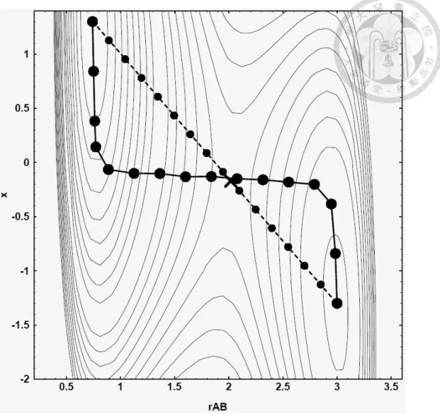
The final validation is the Li diffusion barrier in Si diamond crystal. In order to calculate the dynamical properties, it is crucial to check for the diffusion energy barrier of lithium in silicon. It is calculated by nudged-elastic band (NEB) method. The nudged-elastic band (NEB) method finds the saddle point of the energy surface during reaction. It can be though of as a series of springs in a energy surface and it will finally find the saddle point by the contraction of the spring as shown in figure 4.1.
We tested the diffusion barrier of lithium in silicon𝑇𝑑site to another silicon 𝑇𝑑site by ReaxFF. The silicon cell size is 4 × 4 × 4. We have used 21 images in my calculations.
Figure 4.1 The illustration of the nudge elastic band method
4.2 Structural Properties
The energy volume curve of c-Si, c-LiSi, c-Li12Si7, c-Li13Si4, c-Li15Si4, c-Li22Si5 and c-Li are shown in figure4.2,4.3, 4.4, 4.5, 4.6, 4.7 and 4.8 respectively. We can observed that a smooth energy volume curve is obtained. (by applying the changes in appendix)
−110
−109.5
−109
−108.5
−108
−107.5
−107
17 18 19 20 21 22 23 24
Energy (kcal/mol)
Volume (Å3)
Figure 4.2 The energy volume curve of c-Si
−2600
−2590
−2580
−2570
−2560
−2550
−2540
−2530
−2520
−2510
420 440 460 480 500 520 540 560 580 600
Energy (kcal/mol)
3
−62300
−62250
−62200
−62150
−62100
−62050
−62000
−61950
−61900
−61850
42 44 46 48 50 52 54 56
Energy (kcal/mol)
Volume (Å3)
Figure 4.4 The energy volume curve of c-Li12Si7
−2704
−2702
−2700
−2698
−2696
−2694
−2692
−2690
−2688
−2686
600 650 700 750 800 850
Energy (kcal/mol)
Volume (Å3)
−35100
−35050
−35000
−34950
−34900
−34850
110 115 120 125 130 135 140 145 150
Energy (kcal/mol)
Volume (Å3)
Figure 4.6 The energy volume curve of c-Li15Si4
−456.8
−456.6
−456.4
−456.2
−456
−455.8
−455.6
−455.4
−455.2
120 125 130 135 140 145 150 155 160 165 170
Energy (kcal/mol)
Volume (Å3)
Figure 4.7 The energy volume curve of c-Li22Si5
−254
−253.5
−253
−252.5
−252
−251.5
−251
120 125 130 135 140 145 150 155 160 165 170
Energy (kcal/mol)
Volume (Å3)
Figure 4.8 The energy volume curve of c-Li
The lattice constants of Si, Li and Li–Si alloys calculated by the optimization as described in the previous section are shown as in table 4.1:
We can observe very good agreement of the ReaxFF, DFT and experimental results in lattice constant. The comparison of ReaxFF charge and Bader charge (adopted from Chevrier et al.35) in crystalline Li–Si alloys is shown in table 4.2. The Bader charge in amorphous Li–Si alloys are also calculated in table4.3. The charge of Li in ReaxFF has a value of about the half of the Bader charge. It is closer to the Mulliken charge calculated by Li2O in Gaussian as 0.4 e.
The RDF of a-Li32Si32 by ReaxFF and DFT is compared in figure 4.9, 4.10, 4.11.
While a-Li40Si24and a-Li50Si14are shown in figure 4.12, 4.13, 4.14 and 4.15, 4.16, 4.17
c-Si c-LiSi c-Li12Si7
𝑎( Å) 𝑎( Å) 𝑏( Å) 𝑐( Å) 𝑎( Å) 𝑏( Å) 𝑐( Å) ReaxFF 5.46 9.48 9.48 5.59 8.40 19.95 14.30
DFT 5.46 9.35 9.35 5.75 8.55 19.67 14.33
exp 5.43 9.35 9.35 5.74 8.61 19.74 14.34
c-Li13Si4 c-Li15Si4 c-Li22Si5 c-Li
𝑎( Å) 𝑏( Å) 𝑐( Å) 𝑎( Å) 𝑎( Å) 𝑎( Å)
ReaxFF 7.74 15.45 4.38 10.61 18.61 3.44
DFT 7.92 15.11 4.44 10.62 18.65 3.44
exp 7.99 15.21 4.43 10.69 18.75 3.51
Table 4.1 The lattice constant of Li, Si and their alloys
species Li (ReaxFF) Li(Bader) Si (ReaxFF) Si(Bader)
c-LiSi 0.40 0.77 -0.40 -0.70
c-Li12Si7 0.36 0.76 -0.50 -1.36
c-Li13Si4 0.32 0.73 -1.03 -2.39
c-Li15Si4 0.30 0.80 -1.13 -2.72
Table 4.2 The comparison of ReaxFF and Bader charge of Li in crystalline Li–Si alloy (unit: e)
function. It shows similar peak position in DFT and ReaxFF. However, there are some slight difference between the ReaxFF and DFT data. While focusing on the Li–Li RDF in all concentration, a broader first peak can be observed in the structure. This shows that
species Li (ReaxFF) Li (Bader) Si (ReaxFF) Si (Bader)
a-Li20Si44 0.42 0.83 -0.19 -0.38
a-Li22Si42 0.42 0.83 -0.22 -0.43
a-Li32Si32 0.39 0.82 -0.39 -0.82
a-Li36Si28 0.37 0.82 -0.47 -1.05
a-Li40Si24 0.34 0.81 -0.57 -1.35
a-Li42Si22 0.33 0.81 -0.63 -1.54
a-Li45Si19 0.32 0.80 -0.75 -1.90
a-Li46Si18 0.31 0.80 -0.79 -2.04
a-Li50Si14 0.28 0.79 -1.01 -2.78
Table 4.3 The comparison of ReaxFF and Bader charge of Li in amorphous Li–Si alloy (unit: e)
bonding type cutoff radius
Si–Si 2.8
Si–Li 3.6
Li–Si 3.6
Li–Li 3.9
Table 4.4 The cutoff radius used in the coordination number determiniation
in DFT result. Finally, The Si–Si peak is slightly higher than the DFT Si–Si peak, indicate stronger Si–Si bonding in ReaxFF. The same trend can also be found in the coordination
a-Li32Si32 a-Li40Si24 a-Li50Si14
bonding type ReaxFF DFT ReaxFF DFT ReaxFF DFT
Li–Li 6.88 6.87 9.14 8.54 9.61 10.35
Li–Si 7.46 6.90 5.31 5.21 2.64 2.87
Si–Li 7.46 6.90 8.84 8.68 9.44 10.25
Si–Si 3.38 2.79 2.77 2.13 1.58 0.80
Table 4.5 The coordination number of a-Li32Si32, a-Li40Si24and a-Li50Si14
ume for the optimal lattice constant in NVT 1200 K by ReaxFF and Stillinger Weber po- tential. It shows that the optimal lattice constant in 1200 K is 5.32 Å, while it is 5.46 Å in 0 K optimization as shown in table 4.1. We have tried fully relaxed the structure after 1200 K simulation, which has a lattice constant of 5.32 Å. However, it can not revert back into the lattice constant of 5.46 Å. It can only revert back to up to the lattice constant of 5.38 Å. Besides, the energy for lattice constant as 5.38 Å is unstable when comparing with the silicon structure in the lattice constant of 5.46 Å.
0 1 2 3
1 2 3 4 5
g Li−Li(r)
Distance (Å)
ReaxFF DFT
Figure 4.9 The radial distribution function of Li–Li in a-Li32Si32
0 1 2 3 4 5 6
1 2 3 4 5
g Li−Si(r)
Distance (Å)
ReaxFF DFT
0 1 2 3 4 5 6 7 8
1 2 3 4 5
g Si−Si(r)
Distance (Å)
ReaxFF DFT
Figure 4.11 The radial distribution function of Si–Si in a-Li32Si32
0 1 2 3
1 2 3 4 5
g Li−Li(r)
Distance (Å)
ReaxFF DFT
Figure 4.12 The radial distribution function of Li–Li in a-Li40Si24
0 1 2 3 4 5 6
1 2 3 4 5
g Li−Si(r)
Distance (Å)
ReaxFF DFT
Figure 4.13 The radial distribution function of Li–Si in a-Li40Si24
0 1 2 3 4 5 6 7 8
1 2 3 4 5
g Si−Si(r)
Distance (Å)
ReaxFF DFT
0 1 2 3 4
1 2 3 4 5
g Li−Li(r)
Distance (Å)
ReaxFF DFT
Figure 4.15 The radial distribution function of Li–Li in a-Li50Si14
0 1 2 3 4 5 6 7 8
1 2 3 4 5
g Li−Si(r)
Distance (Å)
ReaxFF DFT
Figure 4.16 The radial distribution function of Li–Si in a-Li50Si14
0 1 2 3 4 5 6 7 8 9 10
1 2 3 4 5
g Si−Si(r)
Distance (Å)
ReaxFF DFT
Figure 4.17 The radial distribution function of Si–Si in a-Li50Si14
−6
−4
−2 0 2 4 6 8 10
5.3 5.35 5.4 5.45 5.5
Pressure (GPa)
Lattice constant (Å)
ReaxFF SW
4.3 Thermodynamical Properties
The formation energy and mixing energy of crystalline Li–Si alloys are plotted as in figure 4.19 and 4.20, while it is plotted as in figure 4.21 and 4.22 for amorphous Li–Si alloys. It is compared with the DFT results. We have also compared our result of crystalline Li–Si alloy with Fan et al.’s data in table4.6.
The crystalline formation and mixing energy shows some deviation from the DFT re- sults, while the amorphous counterparts have similar trend with DFT data. The crystalline formation energy shows good agreement with Fan et al.’s data in table4.6. However, the amorphous alloy has a lower formation or mixing energy than the crystalline counterparts in the 𝑥 range of LixSi and LixSi1-xrespectively. This is shown in figure 4.23 and 4.24.
The energy preference of a-LixSi means that the amorphous structure is more stable than the crystalline structure, which is a problem in the ReaxFF.
bonding type ReaxFF (This work) ReaxFF (Fan et al.) DFT
c-LiSi -14.96 -14.85 -9.30
c-Li13Si4 -86.07 -85.47 -99.75
c-Li15Si4 -95.07 -95.02 -104.84
Table 4.6 The comparison of ReaxFF formation energy with Fan et al.’s data and DFT data. (unt: kcal/mol)
The volume expansion ratio is plotted with DFT data in figure 4.25 and also shows good agreement. We can also observe that the volume of the ReaxFF structure are typicially
The potential energy curve of Si is plotted in figure 4.26 while the potential energy curve of Li is calculated in figure 4.27. An abrupt increase in potential energy means phase transformation and therefore the melting point. We have got a range of 1450–1500 K for silicon while about 450 K for lithium. The experimental value is 1687 K for silicon and 453.65 K for lithium.36It shows good agreement with the experimental data. We have also tested the melting point c-Li12Si7, c-Li13Si4, c-Li15Si4 and c-Li22Si5. However, the c-Li13Si4, c-Li15Si4 and c-Li22Si5 structure collapsed at 400 K and c-Li12Si7 collapsed at 300 K. Even when the structures are not collapsed, the lithium atoms show high mo- bility and diffused off from the equilibrium sites. This shows the instability in the crystal structure, and the agreement with the relative stability of the amorphous and the crystal structures found previously.
−1.6
−1.2
−0.8
−0.4
1 1.5 2 2.5 3 3.5 4 4.5
Formation Energy (eV)
x in LixSi
ReaxFF DFT
−0.4
−0.3
−0.2
−0.1
0.5 0.6 0.7 0.8 0.9
Mixing Energy (eV)
x in LixSi1−x
ReaxFF DFT
Figure 4.20 The mixing energy of c-LixSi
−2.4
−2
−1.6
−1.2
−0.8
−0.4 0 0.4
0 0.5 1 1.5 2 2.5 3 3.5 4
Formation Energy (eV)
x in LixSi
ReaxFF (1200 K MD) DFT
Figure 4.21 The formation energy of a-LixSi