具實驗數據之熱傳導問題的逆向分析 (IV)

科技部補助專題研究計畫報告

具實驗數據之熱傳導問題的逆向分析 (IV)

報 告 類 別 ： 成果報告 計 畫 類 別 ： 個別型計畫

計 畫 編 號 ： MOST 108-2221-E-006-083- 執 行 期 間 ： 108年08月01日至109年07月31日 執 行 單 位 ： 國立成功大學機械工程學系（所）

計 畫 主 持 人 ： 李森墉

共 同 主 持 人 ： 涂德文、吳明勳

計畫參與人員： 碩士班研究生-兼任助理：李慶韋 碩士班研究生-兼任助理：陳彥丞 碩士班研究生-兼任助理：廖永福

本研究具有政策應用參考價值：■否　□是，建議提供機關

（勾選「是」者，請列舉建議可提供施政參考之業務主管機關）

本研究具影響公共利益之重大發現：□否　□是　

中　華　民　國　109　年　10　月　13　日

中 文 摘 要 ： 本報告是多年期計畫的第四年研究結果。整個多年期計畫在於提出 創新的1-D和2-D平板熱傳導問題之正逆向分析方法。其中，逆向方 法結合了解析解、實驗數據與最小均方誤差數值分析。實際的實驗 範例包括: (1)雷射表面加熱問題； (2)噴霧表面散熱問題； (3)矩 形平板具單邊為時變溫度邊界。藉由最小均方誤差法，在比對從物 體內量得到的實驗溫度和從具猜測之時變邊界之熱傳問題(在加熱表 面有未知溫度)的解析解所估算的溫度數據，可求得在受熱端的溫度 函數。據此，在時間和空間內任意點的溫度分佈及熱通量亦均可求 到。數學和實驗的範例將被用來說明本方法的簡單性、有效率以及 準確性，並將同時進行熱傳實驗來驗證。求解方法選用移位函數法

，毋須作任何繁複的積分轉換和逆轉換。本多年期計畫目的在於希 望能解決下列目前大部分的一維和二維熱傳正逆向分析方法存在的 問題： (a)必須處理繁瑣的數值問題，如拉普拉斯轉換、數值分析 的穩定度和含大量元素的矩陣運算； (b)無法同時求得在時間和空 間內任意點的溫度及熱通量； (c)表面加熱處理的時間不可以長 (實驗溫度數據以多項式函數來近似)；(d)加熱處理表面的溫度變化 須緩慢 (實驗溫度數據以多項式函數來近似)； (e)缺乏兩端均為未 知的時變溫度函數問題之逆向熱傳導分析； (f)量測溫度的位置須 非常接近加熱表面； (g)缺乏對多層結構的熱傳導逆向分析；(h)四 邊均具時變邊界條件但四邊角點溫度為零二維矩形平板之正向解析 解。(i)兩邊界絕熱、一邊界等溫及另一邊界具時變二維矩形平板之 正向解析解；(j)四邊均具時變邊界條件且四邊角點溫度亦具時變二 維矩形平板之正向解析解；(k)假設主題(i)之時變邊界未知，配合 實驗量測平板内部多點隨時間變化的温度數值，利用最小平方法作 解析解求得溫度和量測得溫度差平方和之最小值，逆向估算未知邊 界之時變溫度場。加熱方法可為電阻或乙炔焰加熱。

本多年期計畫的前三年已解決上述提到的困難(a-i)。本年計畫則 利用前三年的研究成果，延伸應用求解具時變邊界條件之二維平板 正逆向問題及進行相關熱傳實驗，更深入的探討上述之困難問題(j- k)。

中 文 關 鍵 詞 ： 熱傳導問題正向解析解，熱傳導問題逆向分析，二維矩形平板，時 變邊界條件，最小均方誤差

英 文 摘 要 ： This report is the fourth-year result of a multi-year term research proposal. The methodology proposed uses an

analytic solution, experimental data and numerical analysis for the inverse analysis of 1-D and 2-D plate heat

conduction problems. Experimental data come from the

previous studies on (1) laser surface heating, (2) surface spray cooling problems, and (3) rectangular plates with time-dependent temperature boundary conditions at one end.

By minimizing the mean squares error between the

experimental data obtained from inside the body and the estimated data from the derived analytical solution of the heat conduction problems with guessed time-dependent

temperature boundary conditions (at heating surface with unknown temperature), the unknown temperature function can

be estimated. Consequently, the temperature distribution and the heat flux over the whole time and space domains can also be obtained. The mathematical and experimental

examples will be given to illustrate the simplicity, efficiency, and accuracy of the proposed methodology. The solution method proposed does not require performing any integral transformation and inverse transformation. One expects to overcome the following existing difficulties in the literature: (a) the integral transform and tedious numerical operations, (b) unable to obtain the temperature distribution over the entire time and space domains, (c) the surface heating time cannot be long, (d) the

temperature variation is relatively fast, (e) inverse

analysis with unknown time-dependent boundary conditions at both ends, (f) the temperature measurement point has to be very close to the heating surface, (g) multilayer composite problems, (h) a closed solution for rectangular plates with two insulated boundaries, one constant temperature boundary and one time-dependent temperature boundary, (j) the same physical systems as (h) but with unknown time-dependent temperature at four edges; (k) the same physical systems as (i) but with unknown time-dependent temperature boundary to be estimated. In the first three years, the proposed

methodology has been utilized to overcome the difficulties (a-i) mentioned above. In the fourth year of this plan, we have employed these results obtained in the first three- year to study the direct and/or inverse analysis of 2-D rectangular plates with time-dependent temperature boundary conditions. The proposed problems in issues (j-k) have been investigated in detail.

英 文 關 鍵 詞 ： analytical solution of heat conduction problems, inverse analysis of heat conduction problems, 2-D rectangular plate, time-dependent boundary conditions, minimizing the mean squares error

1

科技部補助專題研究計畫成果報告

（□期中進度報告/▓期末報告）

配合實驗數據之逆向熱傳導問題分析(IV)

Inverse Analysis of Heat Conduction Problems with Experimental Data (IV)

計畫類別：▓個別型計畫 □整合型計畫 計畫編號：MOST 108－2221－E－006－083－

執行期間：108 年 08 月 01 日至 109 年 07 月 31 日

執行機構及系所：國立成功大學機械工程學系(所)

計畫主持人：李森墉

共同主持人：吳明勳、凃德文 計畫參與人員：

碩士班研究生-兼任助理：陳彥丞 碩士班研究生-兼任助理：李慶韋 碩士班研究生-兼任助理：廖永福

本計畫除繳交成果報告外，另含下列出國報告，共 _1_ 份：

□執行國際合作與移地研究心得報告

▓出席國際學術會議心得報告

□出國參訪及考察心得報告

中 華 民 國 109 年 7 月 31 日

I

目 錄

目錄 ………I 摘 要 … … … II Abstract……… III

第一章 前言 ……… 1

第二章 計畫目的 ……… 2

第三章 文獻探討 ……… 4

第四章 研究方法 ……… 7

一、二維熱傳導數學模型 ……… 7

二、二維熱傳導之解析解 ……… 8

1.無因次化 ……… 8

2.疊加原理 ……… 9

3.簡化成一維問題 ……… 11

4.移位函數法……… 11

5.轉換函數之解……… 12

6.解析解 ………13

第五章 結果與討論 ……… 15

一、週期型邊界範例 ……… 15

二、抛物型邊界範例 ……… 18

第六章 結論 ……… 24

參考文獻 ……… 25

附錄 ……… 28

II

摘 要

本報告是多年期計畫的第四年研究結果。整個多年期計畫在於提出創

新的 1-D 和 2-D 平板熱傳導問題之正逆向分析方法。其中，逆向方法結合

了解析解、實驗數據與最小均方誤差數值分析。實際的實驗範例包括: (1)

雷射表面加熱問題； (2)噴霧表面散熱問題； (3)矩形平板具單邊為時變

溫度邊界。藉由最小均方誤差法，在比對從物體內量得到的實驗溫度和從

具猜測之時變邊界之熱傳問題(在加熱表面有未知溫度)的解析解所估算的

溫度數據，可求得在受熱端的溫度函數。據此，在時間和空間內任意點的

溫度分佈及熱通量亦均可求到。數學和實驗的範例將被用來說明本方法的

簡單性、有效率以及準確性，並將同時進行熱傳實驗來驗證。求解方法選

用移位函數法，毋須作任何繁複的積分轉換和逆轉換。本多年期計畫目的

在於希望能解決下列目前大部分的一維和二維熱傳正逆向分析方法存在的

問題： (a)必須處理繁瑣的數值問題，如拉普拉斯轉換、數值分析的穩定

度和含大量元素的矩陣運算； (b)無法同時求得在時間和空間內任意點的

溫度及熱通量； (c)表面加熱處理的時間不可以長 (實驗溫度數據以多項

式函數來近似)；(d)加熱處理表面的溫度變化須緩慢 (實驗溫度數據以多

項式函數來近似)； (e)缺乏兩端均為未知的時變溫度函數問題之逆向熱傳

導分析； (f)量測溫度的位置須非常接近加熱表面； (g)缺乏對多層結構

的熱傳導逆向分析；(h)四邊均具時變邊界條件但四邊角點溫度為零二維矩

形平板之正向解析解。(i)兩邊界絕熱、一邊界等溫及另一邊界具時變二維

III

矩形平板之正向解析解；(j)四邊均具時變邊界條件且四邊角點溫度亦具時 變二維矩形平板之正向解析解；(k)假設主題(i)之時變邊界未知，配合實 驗量測平板内部多點隨時間變化的温度數值，利用最小平方法作解析解求 得溫度和量測得溫度差平方和之最小值，逆向估算未知邊界之時變溫度 場。加熱方法可為電阻或乙炔焰加熱。

本多年期計畫的前三年已解決上述提到的困難(a-i)。本年計畫則利用 前三年的研究成果，延伸應用求解具時變邊界條件之二維平板正逆向問題 及進行相關熱傳實驗，更深入的探討上述之困難問題(j-k)。

關鍵詞：熱傳導問題正向解析解，熱傳導問題逆向分析，二維矩形平板，

時變邊界條件，最小均方誤差

IV

Abstract

This report is the fourth-year result of a multi-year term research proposal.

The methodology proposed uses an analytic solution, experimental data and numerical analysis for the inverse analysis of 1-D and 2-D plate heat conduction problems. Experimental data come from the previous studies on (1) laser surface heating, (2) surface spray cooling problems, and (3) rectangular plates with time-dependent temperature boundary conditions at one end. By minimizing the mean squares error between the experimental data obtained from inside the body and the estimated data from the derived analytical solution of the heat conduction problems with guessed time-dependent temperature boundary conditions (at heating surface with unknown temperature), the unknown temperature function can be estimated. Consequently, the temperature distribution and the heat flux over the whole time and space domains can also be obtained. The mathematical and experimental examples will be given to illustrate the simplicity, efficiency, and accuracy of the proposed methodology.

The solution method proposed does not require performing any integral

transformation and inverse transformation. One expects to overcome the

following existing difficulties in the literature: (a) the integral transform and

tedious numerical operations, (b) unable to obtain the temperature distribution

over the entire time and space domains, (c) the surface heating time cannot be

long, (d) the temperature variation is relatively fast, (e) inverse analysis with

unknown time-dependent boundary conditions at both ends, (f) the temperature

measurement point has to be very close to the heating surface, (g) multilayer

composite problems, (h) a closed solution for rectangular plates with two

insulated boundaries, one constant temperature boundary and one

time-dependent temperature boundary, (j) the same physical systems as (h) but

with unknown time-dependent temperature at four edges; (k) the same physical

systems as (i) but with unknown time-dependent temperature boundary to be

estimated. In the first three years, the proposed methodology has been utilized

to overcome the difficulties (a-i) mentioned above. In the fourth year of this

plan, we have employed these results obtained in the first three-year to study

the direct and/or inverse analysis of 2-D rectangular plates with time-dependent

V

temperature boundary conditions. The proposed problems in issues (j-k) have been investigated in detail.

Keywords: analytical solution of heat conduction problems, inverse analysis of

heat conduction problems, 2-D rectangular plate, time-dependent

boundary conditions, minimizing the mean squares error

1

第一章 前 言

熱傳導逆向問題 (inverse heat conduction problems, 簡稱 IHCPs) 應用 於眾多的工程熱傳問題上，特別是具有難以量測的受熱面溫度或物體表面 熱通量的問題。典型的工程實例，包括：雷射表面加工、熱交換器、燃燒 室、量熱式儀表、砲管內部溫度、金屬加工的快速冷卻和淬火以及電子元 件的冷卻。底下僅限探討雷射表面加工和熱表面的噴灑冷卻問題。

首先，以雷射表面加工問題而言，在雷射表面硬化處理過程，表面溫 度需要維持在臨界轉變溫度且要低於熔點。因此，在熱處理過程中，如何 準確估算表面之溫度以及熱通量表面吸收率極其重要。但由於直接量測加 熱表面的溫度和熱通量相當困難，這些物理量常利用加熱時間內物體內部 的量測溫度資料估算而得。具體而言，此種估算法即為典型的熱傳導逆向 問題。

其次，就熱表面的噴灑冷卻問題而言，其熱表面的表面溫度測試，在 淬火中為最重要的參數，常被用來定義不同熱轉換機制中的沸騰曲線。因 此，在噴灑冷卻過程中，表面溫度和熱通量的估算準確度是相當重要的。

但由於不易直接量測噴灑冷卻表面的溫度和熱通量，這些物理量常由在噴

霧冷卻時間內物體內部的量測溫度資料估算而得。此種估算法亦是典型的

熱傳導逆向問題。

2

第二章 計 畫 目 的

目前有許多數值方法用來解決一維和二維的熱傳導逆向問題，諸如有 限差分法、有限元素法以及邊界元素法等，最常被用來建模以及模擬分析 熱傳導逆向問題。本三年期計畫前二年在於提出創新的一維熱傳導之逆向 分析方法，以解決雷射表面加熱與噴霧表面散熱之工程熱傳問題。而此方 法毋須利用積分轉換，便可求解一維具有時變邊界條件的熱傳導逆向問題。

此外，由於具時變邊界條件二維平板的熱傳廣泛用於眾多工程領域 上，諸如時變加熱於牆壁和平板、雷射加工於固體上、設計透平葉片和自 動引擎之機器零件等為其應用實例。發展具廣義時變邊界條件矩形板之正 向解析解，具有學術研究和工程實務之雙重貢獻。此三年期計畫之第三年 探討內容，係利用已開發之解析解，延伸應用於相關之逆問題分析上。

首先，本多年期計畫之前三年在於解決下列逆向分析方法中所面臨的 七大問題：

(a)必須處理繁瑣的數值問題，如拉普拉斯轉換、數值分析的穩定度和含大 量元素的矩陣運算。

(b)無法同時求得在時間和空間內任意點的溫度及熱通量。

(c)表面加熱處理的時間不可以長(實驗溫度數據以多項式函數來近似)。

(d)加熱處理表面的溫度變化須緩慢(實驗溫度數據以多項式函數來近似)。

(e)缺乏兩端均為未知的時變性溫度函數問題逆向之熱傳導分析。

(f)量測溫度的位置須非常接近加熱表面。

(g)缺乏對多層結構的熱傳導逆向分析。

其中，項次(a)至(d)為第一年已完成之工作重點。具體而言計有:

(1)首先推導具有時變性邊界條件的熱傳導問題之精確解，本法為一種無毋 須採用積分轉換的方法;

(2)進行實驗量測一維除端點外均為絕熱的棒材，在一端或兩端受熱時，内 部三點與端點隨時間變化的温度。加熱方法可為電阻或乙炔焰加熱;

(3)以函數(如：簡易的多項式函數、分段的多項式函數或是傅立葉函數等)

來近似從物體內部所量測到的實驗數據;

3

(4)將具有時變邊界條件的熱傳導問題精確解之時變邊界函數，以上述之相 似未知函數代入。

再者，項次(e)至(g)為第二年已完成之工作重點，計有:

(1)利用第一年之方法，推導具有時變熱通量邊界條件的熱傳導問題之精確 解；

(2)進行實驗量測一維除端點外均為絕熱的棒材，在一端或兩端受熱時，遠 端邊界隨時間變化的温度和熱通量。加熱方法可為電阻或乙炔焰加熱;

(3)以半幅傅立葉餘弦函數來近似從物體邊界量測到的熱通量實驗數據;

(4)將具有時變第二型邊界條件的熱傳導問題精確解之時變邊界函數，以上 述之相似未知函數代入。

此外，項次(h)至(i)為第三年已完成之工作重點，計有:

(h)四邊均具時變邊界條件但四邊角點溫度為零二維矩形平板之正向 解析解。

(i)兩邊界絕熱、一邊界等溫及另一邊界具時變性二維矩形平板之正向 解析解。

最後，本多年期計畫之第四年繼續求解具時變邊界條件之二維平板正逆 向問題及進行相關熱傳實驗。探究主題計有：

(j)四邊均具時變邊界條件且四邊角點溫度亦具時變二維矩形平板之 正向解析解；

(k)假設主題(i)之時變邊界未知，配合實驗量測平板内部多點隨時間

變化的温度數值，利用最小平方法作解析解求得溫度和量測得溫度

差平方和之最小值，逆向估算未知邊界之時變溫度場。

4

第三章 文 獻 探 討

多數逆向熱傳導問題發生在熱傳導狀態下，其對應的邊界條件會造成 其量測上的困難。因此，如何去估算表面溫度與熱通量為大多數學者研究 的課題。而此問題在工程上的具體應用，包括雷射表面加熱、熱交換器、

燃燒室、金屬鑄造快速冷卻與淬火、電子元件冷卻以及表面噴霧等典型例 子。

對於雷射表面加熱問題，據悉雷射表面硬化過程中，其表面溫度必須 維持高於臨界轉變溫度並低於熔點溫度。因此，在加熱過程中，溫度、熱 通量與表面吸收率的精確估算是很重要的。由於直接量測加熱表面的溫度 和熱通量相當困難，這些物理量可由在加熱時間內物體內部的量測溫度資 料估算而得。此外，對於高溫表面噴霧冷卻問題。在噴霧冷卻過程中，熱 表面的表面溫度測試在淬火中為最重要的參數，被用來定義不同熱轉換機 制中的沸騰曲線。因此，在噴灑冷卻過程中，表面溫度與熱通量的估算準 確度同是相當重要的。同樣地，直接量測噴灑冷卻表面的溫度和熱通量相 當困難，而這些物理量可由在噴霧冷卻時間內物體內部的量測溫度資料估 算而得。綜合言之，如何估算上述雷射加工或噴霧冷卻表面溫度，即為典 型的熱傳導逆向問題。

目前有許多數值方法用來解決一維的熱傳導逆向問題。在這些方法

中，有限差分法、有限元素法、邊界元素法是會被來選擇建模和模擬熱傳

導逆向問題數值工具。Lesnic 和 Elliott[1]利用 Adomian’s 分解法來處理紊

亂的輸入數據，得到一個穩定的近似解。Monde 和 Mitsutake [2]，Monde

等人[3]和 Woodfield 等人[4]發展一種解析的方法利用拉普拉斯轉換和有時

間延遲的半級數解去估算一維熱傳導逆向問題的熱擴散率、表面溫度和熱

通量。他們建議選擇接近表面的點來量測以儘可能來做最良好的估算。Hon

和 Wei [5]、Jin 和 Zheng [6]以及 Yan 等人[7]發展一種以網格和積分為架構

的數值方法，利用一個徑向函數求解一維熱傳導逆向問題。然而其矩陣和

方程式過於複雜也很難得到一個準確的結果。對於雷射表面加熱處理問

題，Wang 等人[8]利用一種分析方法包括共軛梯度法作逆向研究，以量測

靠近加熱表面的溫度。他們指出一種合理的方法，藉由兩個不同位置的裝

置來得到表面溫度。Chen 和 Wu [9]則提出一個混合拉普拉斯轉換和有限差

5

分的方法，並配合 Wang 等人[8]在圓柱內測得的實驗數據去預測雷射表面 加熱的溫度。在他們數值的範例中與精確解比較，其估算的熱通量誤差接 近 3%。對於熱表面的噴霧冷卻問題，Qiao 和 Chandra [10]、Cui 等人[11]

利用連續函數方法估算表面熱通量。Hsieh 等人[12]利用暫態液晶技術和熱 電偶去求熱表面噴霧冷卻時的純水之表面溫度參數。Chen 和 Lee [13]利用 混合拉普拉斯轉換和有限差分的方法，配合實驗數據去預測噴霧冷卻表面 的溫度。

上述文獻分析均係針對一維熱傳逆運算問題。對於具有時變邊界條件 之二維熱傳正向問題而言，一些數值技巧已被應用來求解。Zhu [14]、Zhu 等人 [15]、Sutradhar 等人[16]利用拉氏轉換法來處理擴散方程式之時間導 數項，而 Sarler 和 Kuhn [17]則利用有限差分技巧來強化由邊界元素數值法 求得的時域解。此外，Walker [18]利用擴散基本解再結合時域積分以求解 擴散方程式；而 Chen 等人 [19]則應用了修正 Helmholtz 基本解去求解擴散 方程式；Burgess 和 Mahajerin [20]則用基本配置法處理具任意起始條件和 混合時變邊界條件之任意形狀問題；Young 等人[21]直接利用時變擴散方程 式之基本解去求得以擴散運算子基本解線性組合表示之解；Cole 等人 [22]

則涵蓋格林函數法（Green’s function method）以求取矩形平板溫度和熱通 量之快速收斂表達式；Beck 等人[23]則發展具表面加熱條件為時間整數次 方之平板瞬態溫度場。

再者，於進階熱傳教科書[24-26]上，亦可看到透過拉氏轉換法、

Duhemal 理論或格林函數法求解具時變熱傳問題之解析解。首先，當利用 拉氏轉換法，吾人必先於轉換域求得具非齊次邊界條件之二維問題解。如 此一來，在複雜領域轉換解之反拉氏轉換常會發生困難。其次，當利用 Duhemal 理論時，吾人須先求相關非齊性邊界條件之輔助二維問題解 [24:

page 196]。之後，再透過對積分式之微分，方能求得解 [24: page 197]。最 後，就格林函數法 [24: page 217] 而言，則須先導出滿足具單點函數和齊 次邊界條件微分方程式之相應格林函數。又為求得一般解，吾人必須對相 應格林函數取方向微分，再對空間和時間域求作積分。

文獻蒐尋，吾人發現有關二維平板之熱傳逆運算研究非常少見。2001

6

年，Chen 等人 [27]結合拉氏轉換法、具序列及時概念之有限差分法、以 及最小平方法等數值演算法，去預測二維平板之單邊未知表面溫度。應用 相同方法，他們 [28]於隔年預測二維平板之雙邊未知表面溫度。此外，於 2008 年，Chen 和 Wu[29]，再延伸[27-28]相似觀念，並增添溫度量測數據，

去預測二維平板之單邊未知對流熱傳係數。Najafi 等人[30]於 2015 年估算 二維平板之單邊多重熱通量;而於 2017 年，他們 [31]又利用格林函數去求 得二維平板之單邊多重熱通量之正向解析解。

本多年期研究在於發展為一種毋須積分轉換的方法，以求解多維具有 時變邊界的熱傳導正逆向問題。本分析具有時變邊界的熱傳導問題的方法 是由 Lee 和 Lin [32]、Lee 等人 [33]與 Chen 等人[34] 的方法延伸。前三年 計畫已提出創新的一維熱傳導問題之逆向分析方法。探討實際的範例包 括:(1)雷射表面加熱問題與; (2)噴霧表面散熱問題；(3)矩形平板具單邊為 時變溫度邊界。從物體內部所量測到的實驗數據可以利用函數(諸如:簡易 的多項式函數、分段的多項式函數或是傅立葉級數---等等)來近似處理。

藉由最小均方誤差法，在比對從物體內量得到的實驗溫度和從具猜測之時 變邊界之熱傳問題(在加熱表面有未知溫度)的解析解所估算的溫度數據，

可求得在受熱端的溫度函數。也因此，在時間和空間內任意點的溫度分佈

及熱通量亦均可以求得。本方法的簡單性、有效率且準確性，可經由數學

和實驗的各種範例來說明。本第四年研究計畫，係利用前三年對一維及二

維平板熱傳正逆運算結果，將其用於深入探討具時變邊界條件二維平板熱

傳之正逆向問題及執行相關熱傳實驗。底下將針對第(j)項，詳細說明整個

求解方法以及數值分析結果。

7

第四章 研 究 方 法 一、二維熱傳導數學模型

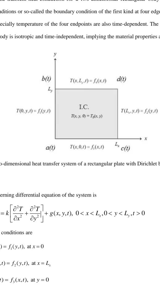
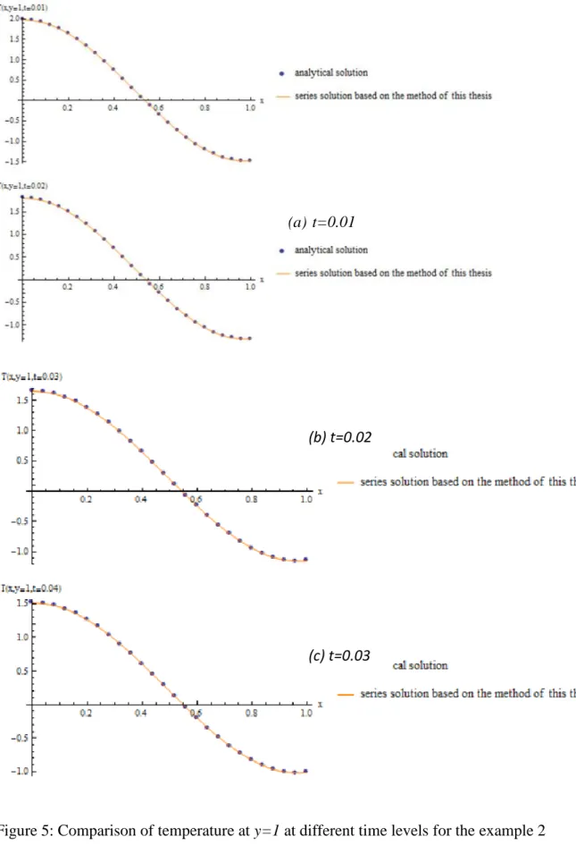
Consider the transient heat conduction for a two-dimensional rectangular body with Dirichlet boundary conditions or so-called the boundary condition of the first kind at four edges, as shown in Figure 1, especially temperature of the four endpoints are also time-dependent. The material of the rectangular body is isotropic and time-independent, implying the material properties are constant.

Figure 1: Two-dimensional heat transfer system of a rectangular plate with Dirichlet boundary conditions

The governing differential equation of the system is

2 2

2 2

( , , ), 0

, 0

, 0

T T T

c k g x y t x L y L t

t x y

 ^  ^^ ^ ^      ⁽¹⁾

the boundary conditions are (0, , ) 1( , ), at 0

T y t  f y t x (2)

( _x, , ) 2( , ), at _x

T L y t  f y t xL (3)

( , 0, ) 3( , ), at 0

T x t  f x t y  (4)

8

( , _y, ) 4( , ), _y

T x L t  f x t at yL (5)

and the initial condition is ( , , 0) 0( , ), 0

T x y T x y at t  (6)

Here, x and y are the space variables and t is the time variable, c is the specific heat, k is the thermal conductivity, T(x, y, t) is the temperature,  is the mass density, Lx and Ly are the thickness of the two-dimensional rectangular body at x and y direction, g(x, y, t) is the heat source inside the rectangular body . For the boundaries, fj (y, t), j = 1, 2 are the general case of temperatures prescribed along the surface at the left end and the right end of the rectangular body. fj (x, t), j = 3, 4 are the general case of temperatures prescribed along the surface at the bottom end and the top end of the rectangular body.

二、 二維熱傳導之解析解

1.

轉換

From the method conducted by Lee [34], there is a restriction that the four endpoints of the plate must be zero. To deal with the restriction, one uses the mathematical technique to enforce the four endpoints to be zero, the transformation is

                   

x y x

x y x

T T a t c t a t b t a t d t b t c t a t

L L L

           

  

  ⁽⁷⁾

where a t( ) is the temperature of endpoint at x=0, y=0, b t( )is the temperature of endpoint at x=0, y=Ly ,c t( )is the temperature of endpoint at x=Lx , y=0,d t( ) is the temperature of endpoint at x=Lx , y=Ly, substituting equation (7) into (1~6), one has the following nonhomogeneous differential equation,

2 2

2 2 ( , , )

T T T

c k g x y t

t X Y

 ^  ^^  ^{ } ⁽⁸⁾

where

9

 

 

( , , ) ( , , )

x y x

x y x

g x y t g x y t c a c a b a d b c a

L L L



            

  

  

  ⁽⁹⁾

in here, a b c d are the differential function of , , ,, , , a b c d with respect to time, the boundary conditions are

(0, , ) 1( , ), 0

T y t  f y t at x (10)

( , , )_x 2( , ), at _x

T L y t  f y t xL (11)

( ,0, ) 3( , ), at 0

T x t  f x t y (12)

( , _y, ) 4( , ), _y

T x L t  f x t at y L (13)

where

     

1( , ) 1( , )

( )

y

f y t f y t a t y b t a t

   L  

 

  ⁽¹⁴⁾

     

2( , ) 2( , )

( )

y

f y t f y t c t y d t c t

L

   

  

  ⁽¹⁵⁾

      

3( , ) 3( , )

x

f x t f x t a t x c t a t

L

    

 

  ₍₁₆₎

4( , ) 4( , ) ( )

( ( ) ( ))

x

f x t f x t b t x

d t b t

   L  

  ⁽¹⁷⁾

and the initial condition is

( , ,0) 0( , ), 0

T x y T x y at t (18)

where

      

            

0( , ) ( , , 0) ^x , 0

y x

a t x c t a t L

T x y T x y at t

y x

b t a t d t b t c t a t

L L

  

  

    

 

 

 

  

  

  

 

(19)

10

2. 疊加原理

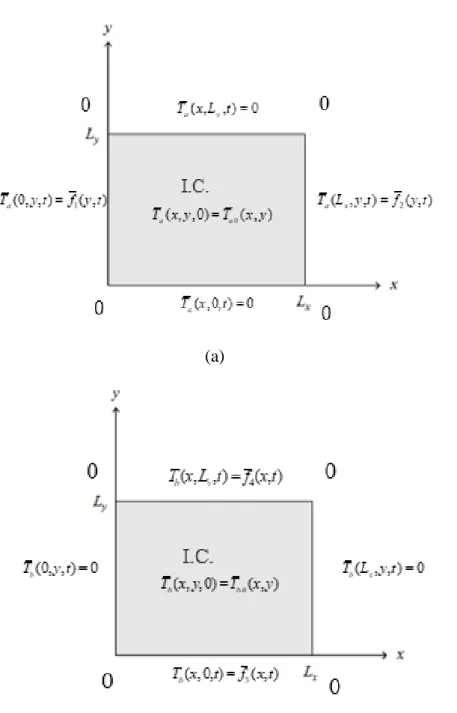
After transformation, since the governing differential equation is linear, one uses the principle of superposition, dividing the equations (8~18) into two parts, which T T_a T_b, gg_a g_b^{, as} shown in Figure 2.

(a)

(b)

Figure 2: The separation subsystems of the two-dimensional heat transfer system with Dirichlet boundary conditions (a) System Ta; (b) System Tb

11

For T_a system governing equation

2 2

2 2 ( , , )

a a a

a

T T T

c k g x y t

t X Y

 ^  ^^  ^ ^  ⁽²⁰⁾

boundary conditions

(0, , ) 1( , ), at 0

Ta y t  f y t x (21)

( , , ) 2( , ), at

a x x

T L y t  f y t xL (22)

( ,0, ) 0, at 0

T xa t  y  (23)

( , , ) 0,

a y y

T x L t  at yL (24)

initial condition

( , ,0) 0( , ), 0

a a

T x y T x y at t (25)

For T_b system governing equation

2 2

2 2 ( , , )

b b b

b

T T T

c k g x y t

t X Y

 ^  ^^ ^ ^ ⁽²⁶⁾

boundary conditions are

(0, , ) 0, at 0

Tb y t  x (27)

( , , ) 0, at

b x x

T L y t  xL (28)

( ,0, ) 3( , ), at 0

T xb t  f x t y  (29)

( , , ) 4( , ),

b y y

T x L t  f x t at yL (30)

initial condition

( , ,0) 0( , ), 0

b b

T x y T x y at t (31)

12

And in terms of the following dimensionless parameters

2 2

0 0

0 0

1 2

1 2

3 3

, , , , , , ,

( , , ) ( , , )

( , , ) , ( , , ) ,

( , ,0) ( , ,0)

( , ,0) , ( , ,0) ,

( , ) ( , )

( , ) , ( , ) ,

( , ) ( , )

y x

a a b b

x y x y y x

a b

a a b b

r r

a b

a b

r r

a a

r r

b

L L

x y t t k

X Y L L

L L L L L L c

T x y t T x y t

X Y X Y

T T

T x y T x y

X Y X Y

T T

f y t f y t

F Y F Y

T T

f x t F X

 

  



   

 

 



      

 

 

 

 ₄ ⁴

2 2

( , )

, ( , ) ,

( , , ) ( , , )

( , , ) , ( , , )

b

r r

a y b x

a a b b

r r

f x t

T F X T

g x y t L g x y t L

G X Y G X Y

kT kT



 



 

(32)

substituting equation (32) into (26~31), one has the following differential equation, For a system

The governing differential equation of the system is

2 2

2

2 2

( , , ) ( , , ) ( , , )

( , , ),

0 1, 0 1, 0

a a a a a a

a a a

a

a

X Y X Y X Y

L G X Y

X Y

X Y

     

 



 

  

  

 









(33)

the boundary conditions are

(0, , ) 1( , ), at 0

a Y a F Y a X

     ⁽³⁴⁾

(1, , ) 2( , ), at 1

a Y a F Y a X

     (35)

( ,0, ) 0, at 0

a X a Y

    ⁽³⁶⁾

( ,1, ) 0, at 1

a X a Y

    (37)

and the initial condition is

0 0

( , ) ( , ,0)

a

r

T x y

X Y T

  (38)

13

For b system

The governing differential equation of the system is

2 2

2

2 2

( , , ) ( , , ) ( , , )

0 1, 0 1,

( , , ),

0

b b b b b b

b b b

b

b

X Y X Y X Y

L G X Y

X Y

X Y

     

 



 

  

  

 

 





(39)

the boundary conditions are (0, , ) 0, at 0

b Y b X

    ⁽⁴⁰⁾

(1, , ) 0, at 1

b Y b X

    (41)

( ,0, ) 3( , ), at 0

b X b F X b Y

     ⁽⁴²⁾

( ,1, ) 4( , ), at 1

b X b F X b Y

     (43)

and the initial condition is

0 0

( , ) ( , ,0) ^b

b

r

T x y

X Y T

  (44)

with the two subsystems, one solves the a system firstly.

3.

簡化成一維問題

As the two opposite edges of the plate, Y=0 and Y=1, are homogeneous boundary conditions, the dimensionless temperature, , and the dimensionless quantity ,

defined in equation (34~35), which can be written respectively as

 

1

( , , ) ( , ) sin

,

a a am a am a

m

X Y X m Y where X

  ^     



 ⁽⁴⁵⁾

   

, 1

1

, 0

( , ) ( ) sin , ( ) 2 ( , ) sin , 1, 2

j a j m a

m

j m a j a

F Y  ^ F  m Y where F  F Y  m Y dY j



     ⁽⁴⁶⁾

  ¹  

0 1

( , , ) ( ) sin , ( , ) 2 ( , , ) sin

a a am a am a a a

m

G X Y  G  m Y where G X  G X Y  m Y dY





    ⁽⁴⁷⁾

For the assumption above, each term of series (45~47) satisfies the boundary conditions. In addition, since the sinusoidal function will construct the orthogonality in its function space. It

14

remains to determine in such a form as to satisfy the boundary conditions on the sides X=0, X=1, and the equation of the governing differential equation as well.

Substituting equations (45~47) into equations (33~35), the following governing differential equation and the non-homogeneous boundary conditions are obtained:

 ^,  ^{2 2}  ₂^,   ,  ( , )

am a am a

a am am a am a

a

X X

L X G X

X

   

   



 

  

  (48)

0,  1, ( ), at 0

am a Fm a X

     (49)

 1, 2, ( ), at 1

am a F m a X

     (50)

where _am 

(

)

To find the solution for the second-order differential equation (48) with non-homogeneous boundary conditions (49~50), one extends the shifting variable method developed by Lee and his colleagues [34], by taking

1, 1, 2, 2,

( , ) ( , ) ( ) ( ) ( ) ( )

am X a am X a Fm a g m X F m a g m X

        (51)

where g_{j m,} ( )X , j=1,2 are shifting functions to be specified, and _am( ,X _a) is the transformed function.

Substituting equation (51) into equations (48~50), which yields the following partial differential equation

2 2

2

1, 2, 2 1, 2,

1, 2, 2 1, 2 2, 2

1, 1, 2, 2,

( ) ( , )

m m m m

am am

m m a m m

a a a

am am m m m m am a

d F d F d g d g

g g L F F

d d X dX dX

F g F g G X

 

  

  

 

    

 

   

 

 

  ⁽⁵²⁾

the associated boundary conditions:

1, 1, 2, 2, 1, , at 0

am F gm m F gm m Fm X

     (53)

1, 1, 2, 2, 2, , at 1

am F gm m F gm m F m X

     (54)

15

4.

移位函數法

To simplify the analysis, the shifting functions are particularly chosen such that they satisfy the following differential equations.

2 ,

2

( ) 0 , 1, 2, 0 1 d gj m X

j X

dX     (55)

and the shifting functions are satisfied the following boundary conditions

, 1, at 0

j m j

g  X  (56)

, 2, at 1

j m j

g  X  (57)

where is the Kroneker symbol. After substituting equations (55~57) into equations (52~54), one

has a differential equation for :

2 2

2 (X, )

am am

a am am am a

a

L G

X

 

  



 

  

  ⁽⁵⁸⁾

where

2

,

, , ,

1

( , ) ( , ) ^{j m}

am a am a am j m j m j m

j a

G X G X F g g d F

   d

 

       

 

 

 

 ⁽⁵⁹⁾

the associated homogeneous boundary conditions:

^0,  ^{0, at 0}

am a X

    (60)

^1,  ^{0, at 1}

am a X

    (61)

and the associated transformed initial condition

    ²

1

0 , ,

0 1

( ,0) 2 , ,0 sin - (0) ( )

am a j m j m

j

X X Y m Y dY F g X

  









These two shifting functions can be easily determined by equation (55~57) as

   

1,_m 1 - , 2,_m

g X  X g X  X (63)