考慮纖維之不可抗壓性的纖維加勁膠墊變形分析

行政院國家科學委員會專題研究計畫 成果報告

考慮纖維之不可抗壓性的纖維加勁膠墊變形分析 研究成果報告(精簡版)

計 畫 類 別 ： 個別型

計 畫 編 號 ： NSC 95-2221-E-011-142-

執 行 期 間 ： 95 年 08 月 01 日至 96 年 07 月 31 日 執 行 單 位 ： 國立臺灣科技大學營建工程系

計 畫 主 持 人 ： 蔡相全

計畫參與人員： 碩士班研究生-兼任助理：廖奕信

處 理 方 式 ： 本計畫涉及專利或其他智慧財產權，2 年後可公開查詢

中 華 民 國 96 年 09 月 27 日

行政院國家科學委員會補助專題研究計畫成果報告 考慮纖維之不可抗壓性的纖維加勁膠墊變形分析

計畫類別：√ 個別型計畫 □ 整合型計畫 計畫編號：NSC 95－2211－E－011－142

執行期間：95 年 8 月 1 日至 96 年 7 月 31 日 計畫主持人：蔡相全

成果報告類型(依經費核定清單規定繳交)：√ 精簡報告 □完整報告

本成果報告包括以下應繳交之附件：

□赴國外出差或研習心得報告一份

□赴大陸地區出差或研習心得報告一份

□出席國際學術會議心得報告及發表之論文各一份

□國際合作研究計畫國外研究報告書一份

處理方式：除產學合作研究計畫、提升產業技術及人才培育研究計畫、列 管計畫及下列情形者外，得立即公開查詢

□涉及專利或其他智慧財產權，□一年√ 二年後可公開查詢

執行單位：國立台灣科技大學營建工程系

中 華 民 國 96 年 7 月 31 日

摘要

利用纖維加勁的彈性層只有在彈性層完全受壓時才可增加其勁度，因為纖維在不受 伸張時會失去其剛性。本研究所建立的纖維加勁彈性層變形分析方法中考慮了此種纖維 加勁僅能承受張力的非線性。除非纖維是在完全張力下，此種非線性纖維加勁會造成壓 力和彎矩的不可分離，而此種不可分離的關係則和纖維受張區的長度有關。增加膠墊承 受的壓力會擴大纖維的張力區並加強膠墊的勁度，但是壓力亦會增加膠墊承受的彎矩進 而擴大膠墊的側向變形。因此考慮纖維加勁僅能承受張力的非線性膠墊，其側屈垂直載 重小於線性纖維膠墊的側屈垂直載重。

關鍵詞﹕橡膠層墊，纖維加勁，隔震。

Abstract

Bonding with fiber reinforcements can increase the stiffness of elastic layers only when the elastic layer is compressed. Fiber loses its rigidity when it is not stretched. The procedure to include this ‘tension-only’ nonlinearity in the deformation analysis of the fiber-reinforced bearing is developed. In the elastic layers bonded with tension-only reinforcements, the responses to the compression force and the bending moment are coupled unless the reinforcements are entirely in tension. The coupled relation, which is not linear, depends on the length of the tension zone in the reinforcement. Increasing the compression force on the bearings will extend the tension zone in the reinforcements and enhance the stiffness of the bearing, but the compression force may add more bending moment to the bearings and increase the lateral deformation. The vertical buckling load of the bearings with tension-only reinforcements varies with the lateral force and is smaller than the buckling load of the bearings with linear reinforcements.

Keywords: Elastomeric bearing; Fiber reinforcement; Seismic isolation.

1. Introduction

A laminated elastomeric bearing consists of elastomeric layers bonded to interleaving reinforcing sheets. High stiffness of reinforcements restrains the lateral expansion of elastomeric layers and results in higher compression stiffness in the vertical direction normal to the layer than an elastomeric layer without bonding to reinforcements. By this characteristic, the laminated elastomeric bearing can provide high vertical rigidity to sustain gravity loading, while still providing the same horizontal flexibility of the elastomer without bonding.

Traditional bearings use steel plates as reinforcement. To analyze the stiffness of the steel-reinforced bearings, the steel reinforcement is treated as completely rigid. The

compression stiffness and tilting stiffness of a single elastomeric layer bonded between two rigid plates have been derived for different shapes of bearings. The simplest approach to solve the stiffness is by assuming the elastomeric layer is an incompressible material (Gent and Lindley, 1959; Gent and Meinecke, 1970; Kelly, 1997). For nearly incompressible materials, such as rubber, the assumption of complete incompressibility tends to overestimate the stiffness of the bonded rubber layer when the shape factor (defined as the ratio of the one bonded area to the force-free area) is high. Including the effect of bulk compressibility can overcome this problem (Chalhoub and Kelly, 1990, 1991; Kelly, 1997). For the compressible elastic layers, there are several stiffness solutions for different shapes of the bearings (Lindley, 1979a, b; Koh and Kelly, 1989; Koh and Lim, 2001; Tsai, 2003, 2005; Tsai and Lee, 1998, 1999), which are suitable for materials of any Poisson’s ratio.

Steel-reinforced bearings are heavy and expensive. Replacing steel reinforcements with fiber reinforcements can significantly reduce both the weight and the cost of bearings (Kelly, 1999, 2002). The fiber reinforcements have high stiffness but cannot be assumed to be completely rigid. The in-plane flexibility of the reinforcements must be considered in the analysis. The compression stiffness and tilting stiffness of the bearings with incompressible elastomeric layers and flexible reinforcements were derived for different shapes (Kelly, 1999;

Tsai and Kelly, 2001, 2002a, b). For the nearly incompressible elastomeric layers, bulk compressibility was included in the stiffness analysis for the fiber-reinforced bearings of the infinite-strip shape (Kelly, 2002; Kelly and Takhirov, 2002). Recently, the compression stiffness of the bearings with compressible elastic layers of any Poisson’s ratio and flexible reinforcements was derived for the infinite-strip shape (Tsai, 2004) and the circular shape (Tsai, 2006).

The fiber reinforcement can provide the in-plane stiffness when it is stretched, but loses the rigidity when compressed. The reinforcement possessing this kind of nonlinear property is referred to as ‘tension-only’ reinforcement here. In the fiber-reinforced bearings, the fiber is stretched when the attached elastic layer is in compression, and is compressed when the attached elastic layer is in tension. Therefore, in the flexural analysis of fiber-reinforced bearings, the deformation of reinforcements is not linear unless the vertical loading of the bearing is so heavy that the elastic layers are entirely in compression. The previous studies on the tilting stiffness of fiber-reinforced bearings do not consider this nonlinear effect and assume the deformation of reinforcements to be linear, which is referred to as ‘linear’

reinforcement here.

In this paper, the effect of bulk compressibility in the elastic layers and the effect of

‘tension-only’ nonlinearity in the reinforcements are considered in the flexural analysis of fiber-reinforced bearings. The reinforcements in the deformed bearing are assumed to remain planar. The bonded elastic layers deform according to two kinematics assumptions: (i) planes parallel to the reinforcements before deformation remain planar after loading; (ii) lines

normal to the reinforcements before deformation become parabolic after loading. The stiffness of a single elastic layer bonded with linear reinforcements is derived first. Then, the method to solve the stiffness of the elastic layer with tension-only reinforcements is developed, which is applied to calculate the displacement of the bearings subjected to the vertical compression and horizontal shear forces. Finally, the stability analysis of the bearings, which includes the shear deformation effect, is carried out.

2. Governing equations

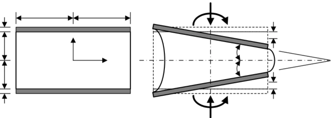
An elastic layer in the infinite-strip bearing, which has a width of 2b and a thickness of t, is shown Fig. 1. The top and bottom surfaces of the elastic layer are perfectly bonded to flexible reinforcements of thickness t . A local coordinate system (x, y, z) is located at the _f center of the elastic layer. The y-axis is attached to the infinite-long direction. The length of the bearings of infinite-strip shape is much larger than the other dimensions, so that the deformation of the bearing is assumed to be in plane strain state and only a unit length of the bearing is analyzed. Under a compression force P and a pure bending moment M, the thickness of the elastic layer is reduced byΔ ; the top and bottom reinforcements rotate to form an angleφ. The displacements of the elastic layer along the x and z directions, denoted as u and w respectively, are assumed to have the form

) ( 4 )

1 )(

( ) ,

( _{2 1}

2

0 u x

t x z u z x

u = − + (1)

t x z z

x

w( , )=−(Δ+φ ) (2)

in which u₁ represents the horizontal displacement of the reinforcements; the term of u ₀ represents the additional bulging or shrinking displacement in the elastic layer which is assumed to be parabolic. The vertical displacement in Eq. (2) fulfills the assumption that planes parallel to the reinforcements remain planar.

For isotropic elastic layers, the mean pressure p has the following relation with the displacements

) (

) ,

(x z u_,x w_,z

p =−κ + (3)

where κ is the bulk modulus of the elastic layer, and the commas imply differentiation with respect to the indicated coordinate. The effective pressure p is defined as

∫

= ^/2

2

/ ( , )

) 1

( ^t

t p x z dz

x t

p (4)

which becomes, when using the displacement assumptions in Eqs. (1)-(2),

t x u t

p u

x x

φ

κ ⁺

+ Δ

−

−

= _{0, 1,} 3

2 (5)

By the principle of virtual work,

∫ ∫

= +

Δ ^b

b t

t zz zzdzdx

M

P ^/2

2

/ σ δε

δφ

δ (6)

where σ , the normal stress of the elastic layer in the z direction, has the form _zz

⎟⎠

⎜ ⎞

⎝

⎛ +

− −

= + _z

zz E p w

2 ,

1

1 ν κ

ν

σ ν (7)

with E and ν being the elastic modulus and Poisson’s ratio of the elastic layer, respectively.

Since the virtual strain is

(

)

δε x

zz =−1t Δ+

(8) the compression force and bending moment acting on the elastic layer become

∫

−

= ^b

b zzdx

P σ (9)

∫

−

= ^b

b zzxdx

M σ (10)

where σ is the effective vertical stress defined as _zz

⎟⎠

⎜ ⎞

⎝

⎛ +Δ+

−

− +

=

=

∫

t t p dz E

z t x

x ^t

t zz

zz

φ κ

ν ν σ ν

σ 1 ( , ) 1 1 2

)

( ^/2

2

/ (11)

Integrating the equilibrium equation of the elastic layer in the x direction through the thickness of the elastic layer leads to

⎟⎠

⎜ ⎞

⎝

⎛− +

−

= −

u t t

p_x φ

ν ν

κ ^{2 0}

, 8

) 1 ( 2

2

1 (12)

The boundary condition of the normal stress at the edge of the elastic layer is σ_xx(± zb, )=0. Substituting Eq. (1) into this boundary condition and then integrating through the thickness of the layer gives

⎟⎠

⎜ ⎞

⎝⎛ ±Δ

−

= −

±

b t t b

p φ

ν ν

κ 1

2 1 )

( (13)

The thickness of the reinforcements is much smaller than the thickness of the elastic layers, so that the stress in the reinforcements can be regarded as being in plane stress state within x-y plane. Let N be the normal force in the x direction acting on a unit length of the _xx reinforcement which has the following relation with the displacement of the reinforcement

) 1 (

)

( E t₂ u_1, x x

N _x

f f f

xx = −ν (14)

with E and _f ν_f being the elastic modulus and Poisson’s ratio of the reinforcement,

respectively. The internal forces acing on the reinforcement have the following equilibrium equation (Tsai, 2004)

0 ) 2 / , ( ) 2 / ,

, + (x−t − x t =

N_xxx τ_xz τ_xz (15)

where )τ_xz(x,−t/2 and τ_xz( tx, /2) are the bonding shear stresses generated by the elastic layers bonded to the top and bottom, respectively, of the reinforcement. Eq. (15) can be revised, from Eqs. (1), (2) and (12), as

⎟⎟⎠

⎜⎜ ⎞

⎝

⎛ −

−

−

= +

t Et p

N_xxx ^x φ

κ ν ν ν

,

, 1 2

1

1 (16)

Integrating Eq. (16) from x to b and using the boundary conditions N_xx(b)=0 and p(b) in Eq. (13) lead to

⎟⎠

⎜ ⎞

⎝

⎛ −Δ−

−

−

= + x

t t p

N_xx Et φ

κ ν ν ν 1 2

1

1 (17)

The shape factor of the bonded elastic layer in infinite-strip shape is defined as t

S = (18) b

The ratio of the elastic layer stiffness to the reinforcement stiffness is defined as

f f

f

t E R Et(1−ν²)

= (19)

Substituting u_0,x, obtained from Eq. (12), and u_1,x, obtained from Eqs. (14) and (17), into Eq.

(5) leads to

⎟⎠

⎜ ⎞

⎝⎛ +Δ

⎟⎠

⎜ ⎞

⎝

⎛ + +

−

− −

=

− x

t t R b

S

p_xx p φ

ν ν

ν α κ

κ 1 1

1 2 6 ₂ 1

2 2

, (20)

with

⎟⎠

⎜ ⎞

⎝

⎛

+ +

−

= −

ν ν

α ν

1 1

2

6 1 R

b

S (21)

The solution of Eq. (20) has a general form

⎟⎠

⎜ ⎞

⎝⎛ +Δ

⎟⎟⎠

⎜⎜ ⎞

⎝

⎛ + −

− + − +

= x

t t b x S

B x

p A φ

α ν

ν ν

α ν

κ α ^{2 2}

2

) 1 ( 1 6 1

2 sinh 1

cosh (22)

where A and B are constants determined from the boundary conditions of p . 3. Solutions for linear reinforcements

The solutions derived in this section are applicable to bearings with reinforcements which

can sustain tension and compression forces and have compression stiffness equal to tension stiffness, referred to as ‘linear’ reinforcements here. Using the boundary conditions p( b− ) and p(b) shown in Eq. (13), the solution of p in Eq. (22) can be derived. Then, substituting this derived p into Eq. (11) gives

⎥⎦

⎢ ⎤

⎣

⎡ ⎟

⎠

⎜ ⎞

⎝

⎛Δ +

+ −

⎟⎠

⎜ ⎞

⎝⎛ +Δ

⎟⎟⎠

⎜⎜ ⎞

⎝

⎛ + −

− −

= b

x t

b b x t

b x S

t t b S E

zz α

α φ α α α

ν ν φ

α ν ν σ ν

sinh sinh cosh

cosh )

1 (

6 )

1 ( 1 6

1 ^{2 2}

2 2 2

2 2 2

2 (23)

from which, using Eqs. (9)-(10), the compression force and bending moment are found as

⎥⎦

⎢ ⎤

⎣

⎡ ⎟

⎠

⎜ ⎞

⎝⎛ − + −

−

= Δ

b b b

S t

Eb P

α α α

ν ν ν

1 tanh )

1 ( 1 6 1

2 1 _{2 2}

2 2

2 (24)

⎭⎬

⎫

⎩⎨

⎧ ⎥

⎦

⎢ ⎤

⎣

⎡ ⎟

⎠

⎜ ⎞

⎝

⎛ −

− −

− +

= 1

tanh )

( 1 3 )

1 ( 1 6 1

1 3

2

2 2

2 2 2 2

2 b

b b

b b S

t Eb

M

α α α

α ν ν ν

φ (25)

which indicate that compression force and bending moment are not coupled. The compression force is only related to thickness reduction, while the bending moment is only related to sectional tilting.

Using Eq. (17), the normal force in the reinforcement can be found as

⎥⎦

⎢ ⎤

⎣

⎡ ⎟

⎠

⎜ ⎞

⎝⎛ −

⎟+

⎠

⎜ ⎞

⎝⎛ −

− Δ

= b

x b

b x b x b

S N_xx E

α φ α

α α α

ν ν

sinh sinh cosh

1 cosh )

1 (

6

2 2 2

2

(26) Fig. 2 plots the distributions of σ_zz and N along the x-axis for different deformation ratios _xx

) /(bφ

Δ , which shows that, when Δ/(bφ)<1, part of the effective vertical stress in the elastic layer is in tension which creates compression force in the reinforcement.

4. Solutions for tension-only reinforcements

The solutions derived in this section are applicable to the bearings with the reinforcements which only have tension stiffness to sustain tension force, but do not have any rigidity to sustain compression force, referred to as ‘tension-only’ reinforcement here. When the elastic layer is under compression in the vertical direction, the attached reinforcements are stretched in the horizontal direction and create the constraint effect on the elastic layer, whereas, when the elastic layer is under tension in the vertical direction, the attached reinforcements are shortened in the horizontal direction and do not have any constraint effect on the elastic layer.

Considering the deformation shown in Fig. 1, denote c as the x-coordinate of the starting point from which the reinforcement is subjected to tension in c<x<b. In −b<x<c, the normal force in the tension-only reinforcements becomes N_xx =0, so that Eq. (17) becomes

⎟⎠

⎜ ⎞

⎝⎛ +Δ

−

= − x

t t

p φ

ν ν κ 1

2

1 (27)

Substituting this into Eq. (11) gives the effective vertical stress in −b<x<c as

⎟⎠

⎜ ⎞

⎝⎛ +Δ

− −

=

− x

t t E

zz

φ

σ ν₂

1 (28)

From Eq. (27), it is known

⎟⎠

⎜ ⎞

⎝⎛ +Δ

−

= − c

t t c

p φ

ν ν

κ 1

2 1 )

( (29)

Based on this equation and p(b) in Eq. (13), the solution of p in Eq. (22) for c<x<b can be derived. Using the derived p , the effective vertical stress defined in Eq. (11) has the form in c<x<b as

⎭⎬

⎟⎫

⎠

⎜ ⎞

⎝⎛ +Δ

⎥⎦

⎢ ⎤

⎣

⎡ + −

−

⎩⎨

⎧ ⎥

⎦

⎢ ⎤

⎣

⎡

−

⎟ −

⎠

⎜ ⎞

⎝⎛ +Δ

− +

⎟ −

⎠

⎜ ⎞

⎝⎛ +Δ

−

= −

+

t x t b S

c b

x c b

t t c b

c b x

t t b S E

zz

φ α

ν ν

α α φ

α α φ

α ν ν σ ν

2 2 2 2 2 2 2 2 2

) 1 ( 1 6

) ( sinh

) ( sinh )

( sinh

) ( sinh )

1 (

6 1

(30)

From Eq. (17), the normal force of the reinforcement in c<x<b is

⎭⎬

⎥⎫

⎦

⎢ ⎤

⎣

⎡

−

− −

−

− − +

⎩⎨

⎧ ⎥

⎦

⎢ ⎤

⎣

⎡

−

− −

−

− −

− Δ

=

) ( sinh

) ( sinh )

( sinh

) ( sinh

) ( sinh

) ( sinh ) ( sinh

) ( 1 sinh )

1 (

6

2 2 2

2

c b

x b b

c c b

c x b

b x

c b

x b c

b c x b

S N_xx E

α α α

φ α

α α α

α α

ν ν

(31)

According to Eqs. (9)-(10), the compression force and bending moment can be found by

⎟⎠

⎜ ⎞

⎝⎛ +

−

=

∫

∫

− b

c zz c

b zzdx dx

P σ σ (32)

∫

∫

− +

= ^b

c zz c

b zzxdx xdx

M σ σ (33)

which give the matrix form as

⎪⎪

⎭

⎪⎪

⎬

⎫

⎪⎪

⎩

⎪⎪

⎨

⎧ Δ

⎥⎥

⎦

⎤

⎢⎢

⎣

=⎡

⎪⎪

⎭

⎪⎪

⎬

⎫

⎪⎪

⎩

⎪⎪

⎨

⎧

t b t a a

a a

Eb M Eb

P

2 φ

3 3 1

2

(34)

with

⎥⎦

⎢ ⎤

⎣

⎡

−

−

− −

− − + −

= −

) ( sinh

1 ) ( 2cosh 1

) )( 1 )(

1 (

6 1

2 2

2 2 1 2

c b b

c b b

c b

a S

α α

α α

ν ν

ν

ν ⁽³⁵⁾

⎥⎥

⎥⎥

⎦

⎤

⎢⎢

⎢⎢

⎣

⎡

−

−

−

− + + −

− − + −

= −

) ( sinh

2 ) ( cosh ) 1 ( ) 3 (

1 3 1

) )( 1 )(

1 (

2 )

1 ( 3

2 ²

2

2 3

3 2 2

2 2 2

c b b

b c c b b

c b

b c b

c b

a S

α α

α α

α ν ν

ν

ν ⁽³⁶⁾

⎥⎦

⎢ ⎤

⎣

⎡

−

− + −

−

− −

= −

) ( sinh

1 ) ( )cosh 1

( 2 1

) )( 1 )(

1 (

3

2 2 2 2

2

3 b b c

c b b

c b

c b

a S

α α

α α

ν ν

ν (37)

It should be noted that the solution presented in this section is based on the tilting deformation shown in Fig. 1 where the reinforcements are subjected to tension in c<x<b, so that the tilting angle φ must always be positive, but the thickness reduction Δ can be positive or negative.

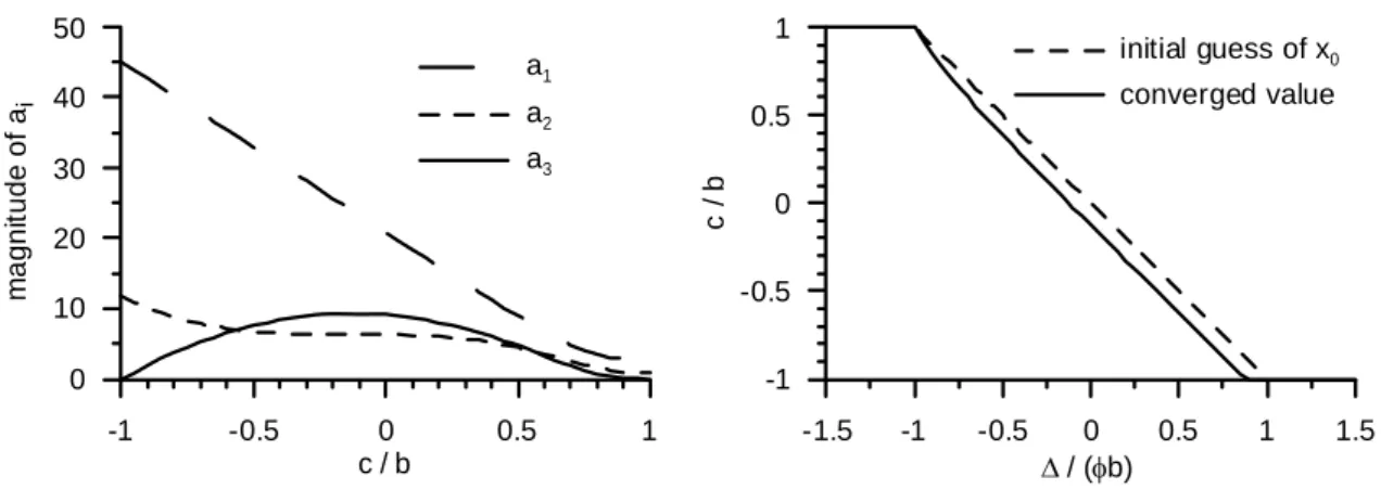
The variations of the coefficients a with the starting point c are plotted in Fig. 3(a) for _i the bearing which hasS =20,R=0.01and ν =0.495. The tension zone of the reinforcement is reduced when the c value is moving from –b to b, which leads the magnitudes of a₁ and

a2 decrease. The magnitude of a has a larger value near ₃ c=0 and becomes zero at b

c=± . When c=−b, the reinforcements are fully in tension; Eq. (34) becomes the same as the force-deformation relation of the elastic layer with linear reinforcements in Eqs. (24)-(25).

When c=b, the reinforcements do not sustain any tension; Eq. (34) becomes t

Eb

P Δ

= − ₂ 1

2

ν ⁽³⁸⁾

t b Eb

M φ

ν ) 1 ( 3

2

2

2 = − (39)

which is the force-deformation relation of the elastic layer without reinforcement. When b

c b< <

− , 0a₃ ≠ means that compression force and bending moment are coupled with thickness reduction and sectional tilting.

The force-deformation relation in Eq. (34) is not linear, because the starting point c shown in the coefficients a of the stiffness matrix is varied with the deformations _i Δ and φ. An iteration scheme must be applied to find the starting point c for the given Δ and φ. The iteration is initiated by setting c⁽¹⁾ =−b and applying the Newton-Raphson method on Eq. (31) to find the root x so that ₀ N_xx(x₀)=0 for the corresponded staring point c⁽¹⁾. The next iteration is carried out by setting c⁽ⁱ⁺¹⁾ =(c⁽ⁱ⁾ +x₀)/2 until the value of c converges. In each iteration, an initial guess for x is required when using the ₀ Newton-Raphson method to find the root x . The following initial guess for the ₀ Newton-Raphson method is applied

φ φ φ

φ φ

b b b

b

b b x

≥ Δ

<

Δ

<

−

−

≤ Δ

⎪⎩

⎪⎨

⎧

− Δ

−

=

if if if

0 / (40)

Fig. 3(b) plots the initial guess of x and the converged value of c as functions of the ₀ deformation ratio Δ/(bφ), which indicates that the initial guess of x₀ can be treated as the upper bond of the starting point c.

Using the solved starting point c, the distributions of σ and _zz N along the x-axis for _xx different deformation ratios Δ/(bφ) are plotted in Fig. 4, which shows that the reinforcement is subjected to tension at the place where the effective vertical stress of the elastic layer is negative; the small positive σ exits at the place where _zz N_xx =0.

Since the staring point c is fixed for a particular deformation ratio Δ/(bφ), the coefficients a are not changed as long as the ratio of _i Δ/t to b /φ t is the same. In other words, when the deformations Δ/t and b /φ t are changed by the same scale, the forces

) /(Eb

P and M /(Eb²) will be linearly varied with the same scale.

The variations of compression force and bending moment with thickness reduction for a fixed tilting angle are plotted in Fig. 5. When Δ≥bφ, the bending moment is constant and the compression force linearly reduces the thickness like an elastic layer with linear reinforcements. When Δ≤−bφ, the bending moment is constant and the tension force linearly increases the thickness like an elastic layer without reinforcement. Therefore, when

=0

φ , the curve of compression force becomes bilinear and the curve of bending moment is

=0 M .

The variations of bending moment and compression force with tilting angle for a fixed thickness reduction are plotted in Fig. 6. When Δ=0, the constant deformation ratio,

0 ) /( =

Δ bφ , gives the fixed c point which means the coefficients a are constant, so that the _i curves for Δ=0 are linearly varied with φ . When Δ t/ =1 and bφ/t ≤1 , the compression force is constant and the bending moment linearly varies with the tilting angle like an elastic layer with linear reinforcements. When Δ t/ =−1 and bφ/t ≤1, the tension force is constant and the bending moment linearly varies with the tilting angle like an elastic layer without reinforcement.

To check the accuracy of the proposed solution procedure, a nonlinear finite element analysis on a bearing of 20 elastic layers has been carried out. In the finite element analysis, each elastic layer is modeled by four layers of the 4-node plane-strain elements with incompatible bending modes. The reinforcement is modeled by the bilinear elastic bar elements which have zero stiffness in compression. The results of the finite element analysis are plotted in Fig. 4 to Fig. 6, which indicates that the solutions of the proposed procedure are

consistent with the finite element solutions.

From Eq. (34), the deformation of elastic layer can be expressed in terms of the applied force and moment,

⎪⎪

⎭

⎪⎪

⎬

⎫

⎪⎪

⎩

⎪⎪

⎨

⎧

⎥⎥

⎦

⎤

⎢⎢

⎣

⎡

−

−

= −

⎪⎪

⎭

⎪⎪

⎬

⎫

⎪⎪

⎩

⎪⎪

⎨

⎧ Δ

2 1

3 3 2

2 3 2

1 )

( 1

Eb M Eb

P

a a

a a

a a b a

t t

φ (41)

A similar iteration scheme can be applied to calculate Δ and φ. The iteration is initiated by setting c⁽¹⁾ =−b and calculating the corresponded coefficients a from Eqs. (35)-(37) for _i the corresponded staring point c⁽¹⁾. Then Δ and φ from Eq. (41) are calculated, which will be applied in Eq. (40) to set the initial guess x for solving ₀ N_xx(x₀)=0 by the Newton-Raphson method. The next iteration is carried out by setting c⁽ⁱ⁺¹⁾ =(c⁽ⁱ⁾ +x₀)/2 until the value of c converges.

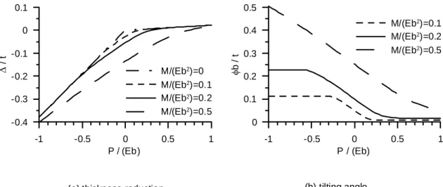
The variations of thickness reduction and tilting angle with compression force for a fixed bending moment are plotted in Fig. 7. The variations of tilting angle and thickness reduction with bending moment for a fixed compression force are plotted in Fig. 8. These figures indicate that increasing the compression force will shorten the thickness of the elastic layer and reduce the tilting angle, and increasing the bending moment will enlarge the thickness of the elastic layer and increase the tilting angle.

5. Flexural analysis of bearings

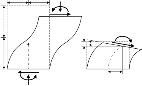
The deformation of an infinite-strip bearing of height H =2h , which consists of multiple elastic layers of width 2b interleaving with reinforcements, is shown in Fig. 9. The bottom of the bearing is fixed against any displacement and rotation, whereas the top of the bearing is allowed to move horizontally and vertically but is still constrained against rotation.

The top of the bearing is subjected to a horizontal shear force F and a vertical compression force P. The ζ -axis denotes the centroidal axis of the bearing in the vertical direction with the origin located at the bottom of the bearing. Deformation of the bearing can be described by the three variables: the horizontal displacement υ and the vertical displacement ω of the centroidal axis, and the rotation angle ψ of the cross-section. Since the thickness of an elastic layer is much smaller than the height of the bearing and is much larger than the thickness of the reinforcement, the deformation of the bearing can be treated as a homogenous column by using the following equivalent relation with the deformation of the elastic layer:

t d

d Δ

ζ ≈

ω (42)

t d

d φ

ζ

ψ ≈ (43)

The shear stiffness of the bearing used for seismic or vibration isolation is usually much less than the compression stiffness or the resistance of bending, so that the shear deformation has to be considered in the deformation analysis of the bearing. The slope of the deformed column axis is equal to the summation of the rotation of the cross-section ψ and the angle of shear deformation γ

γ ζ ψ

υ = + d

d (44)

The constitutive equation for the shear force V is γ

GA

V = (45)

where )G=0.5E/(1+ν is the shear modulus of the elastic layer and A=2b is the cross-sectional area. Substituting Eq. (45) into Eq. (44) and using V =F yield

GA F d

d =ψ + ζ

υ (46)

Since the lateral deformation of the bearing is anti-symmetric to the middle height of the bearing )(ζ =h where dψ dζ =0 and the bending moment M =0, the bending moment acting at the ends of the bearing is

Fh

M₀ = (47)

The bending moment in the bearing can be expressed as ζ

F M

M = ₀ − (48)

The first-order differential equations in Eqs. (42), (43) and (46) for the three dependent variables υ , ψ and ω can be solved by numerical method. The values of Δ/t in Eq.

(42) and φ/t in Eq. (43) are calculated from Eq. (41) by using the bending moment M in Eq.

(48).

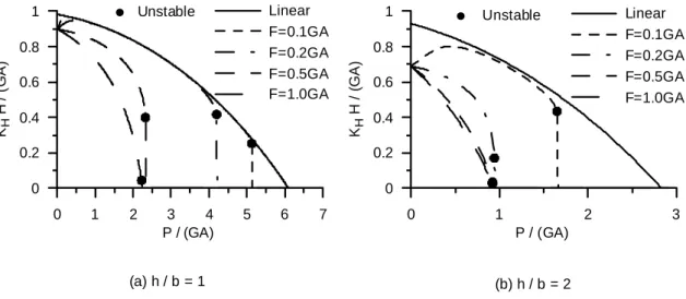
The deformation of the bearings with tension-only reinforcements are solved by the fourth-order Runge-Kutta method with the step size h/50. The vertical displacement at the top of the bearing and the rotational angle of the cross-section at the middle height of the bearing are shown in Fig. 10 as a function of the compression force. The ω value is positive when the vertical displacement is downward. The negative ω value shown in the cases of the smaller compression force indicates that the center of the bearing is uplifted. The cross-section rotation is reduced by increasing the compression force, because the tension zone in the reinforcement is increased and the bearing becomes stiffer. The same phenomenon can also be observed in Fig. 11 where the horizontal displacement at the top of the bearing and the lateral stiffness of the bearing, defined as K_H =F/υ(H), are plotted as a function of the compression force. Figure 11 shows that the bearing has smaller lateral