An Adaptive Nearest Neighbor Classifier Based on Nonparametric Separability

(1)

An Adaptive Nearest Neighbor Classifier Based on Nonparametric Separability

Hsin-Hua Ho

¹

Cheng-Hsuan Li

²

Bor-Chen Kuo

³

ABSTRACT

A k-nearest-neighbor classifier expects the class conditional probabilities to be locally constant.

In this paper, we use the local separability based on nonparametric weighted feature extraction criterion to establish an effective metric for computing a new neighborhood. For each test pattern, the modified neighborhood shrinks in the direction with high separability around this pattern and extends further in the other direction. This new neighborhood can often provide improvement in classification performance. Therefore, any neighborhood-based classifier can be employed by using the modified neighborhood. Then the class conditional probabilities tend to be more homogeneous in the modified neighborhood.

Key Words: pattern recognition, classifier, k-nearest-neighbor (kNN) classifier,

nonparametric weighted feature extraction (NWFE)

1. Introduction

The k-nearest-neighbor (k-NN) classifier is a simple and appealing classifier. When a new sample arrives, k-NN finds the k neighbors nearest to the new sample from the training space based on some suitable similarity or distance metric. A common similarity function is based on the Euclidian distance between two data. k-NN is based on the assumption that locally the class posterior probabilities are approximately constant. However, when an unclassified sample point is near the decision boundary, the class conditional probability of the new sample is not approximately constant.

Therefore, this new sample may probably be labeled incorrect (Hastie and Tibshirani, 1996).

During the past decade various choices of the more suited distance metric have been

investigated to compute the neighborhood. The DANN (discriminant adaptive nearest neighborhood classification) metric, proposed by Hastie and Tibshirani (Hastie and Tibshirani, 1996) for the k-NN classification task is one of the well-known software packages using the separability of linear discriminant analysis (LDA).

In this paper, we create a new metric based on the separability from nonparametric weighted feature extraction (NWFE) (Kuo and Landgrebe, 2004; Fukunaga, 1990). For each test pattern, the modified neighborhood shrinks in the direction with high separability and extends further in the other direction. In two dimension case, it is easy to image that we shrink an original neighborhood in direction approximately orthogonal to the decision boundary, and elongate it approximately parallel

Received Date: Sep. 14, 2007 Revised Date: Nov. 30, 2007 Accepted Date: Dec. 03, 2007 1 Ph. D. Student, Department of Electrical Engineering, National Chung Hsing University

2 Ph. D. Student, Department of Electronic & Control Engineering, National Chiao Tung University

3 Professor, Department of Graduate School of Educational Measurement and Statistics, National Taichung University

(2)

to the boundary. Then the class conditional probabilities tend to be more homogeneous in our method.

The paper is organized as follows. We begin with a review of the nonparametric weighted feature extraction (NWFE) in Section 2. In Section 3, we present our k-nearest neighbor classifier based on adaptive nonparametric separability. The special case using whole training samples of our method is studied in Section 4. The effectiveness of the proposed method is experimentally verified in Section 5. Finally, in the last section, we give the concluding comments.

2. Nonparametric Weighted Feature Extraction

The main ideals of the nonparametric weighted feature extraction (NWFE) are putting different weights on every sample to compute the "weighted means" and compute the distance between samples and their weighted means as their "closeness" to boundary, then defining nonparametric between-class and within-class scatter matrices which put large weights on the samples close to the boundary and de-emphasize those samples far from the boundary. The between-class scatter matrix Sb^NW and the within- class scatter matrix Sw^NW of NWFE are defined as

, )) ( ))(

(

( ⁽⁾ ⁽⁾ ⁽⁾ ⁽⁾

1 1 1

) , (

T i k j i k i k j i k L

i L

i jj

n

k i

j i i k NW

b x M x x M x

P n

S =

∑ ∑∑

ⁱ − −

= ≠= =

λ

, )) ( ))(

( (

1 1

) ( ) ( ) ( ) ( ) ,

∑ ∑

(

= =

−

= ^L

i n k

T i k i i k i k i i k i

i i k i NW w

i x M x x M x

P n

S λ

where ⁽ ⁾ ^,

1 ) ( ) , ( )

(

∑

=

= ^j

n l

j l j i kl i

k

j x w x

M

, )) ( ( dist

)) ( ( dist

1

1 ) ( ) (

1 ) ( ) ( )

(

∑

=

−

=

ni

l

i l j i l

i k j i i,j k

k

x ,M x

x ,M

λ x ,

) ( dist

1

1 ) ( ) (

1 ) ( ) ( )

(

∑

=

−

= ni

l

j l i k

j l i k i,j

kl

,x x

,x w x

n_i denotes the training sample size of class i,

) ( ⁽ⁱ_k⁾

j x

M denotes the weighted mean of x⁽ⁱk⁾ in class j, L is the number of classes and^dist⁽^x^,^z⁾ be the Euclidean distance from^x to ^z.

The goal of NWFE is to find a linear transformationA∈R^d^×^p, ^p^≤^d, which maximizes the between-class scatter and minimizes the within-class scatter. The columns of ^A are the optimal features by optimizing the following criterion,

) )

( tr(

max

arg A S A ¹A S A

A ^T _w^NW ^T _b^NW

A

= − .

This maximization is equivalent to find eigen-pairs (λ_i,v_i),i=1,2,L,d , λ1≥λ2≥L≥λ_d for the generalized eigenvalue problem

v S v

S_b^NW =λ _w^NW .

3. K‐Nearest‐Neighbor Classifier Based on a Novel Metric Using Adaptive NWFE

Separability

In the standard k-NN classifier, the Euclidean distance is used to measure the similarity of unclassified pattern and training samples. Instead of the Euclidean distance, sometimes we could also use the Mahalanobis distance. The Mahalanobis distance between the unknown pattern x*and the training sample x⁽ⁱj⁾

is defined as

),

* ( )

*,

(x x⁽_jⁱ⁾ x x⁽_jⁱ⁾^TC¹ x x⁽_jⁱ⁾

d = − ⁻ −

where C⁻¹ denotes the inverse covariance matrix estimated by the whole training samples.

(3)

In our experiments, kNN-MD means the k-NN classifier using the Mahalanobis distance.

In this section, a k-nearest-neighbor classifier based on a novel metric using adaptive nonparametric separability (kNN-ANS) is proposed. This technique is based on the exploitation of the results of the nonparametric weighted feature extraction (NWFE) performed on a set of Kmpatterns in a nearest neighborhood of unclassified pattern x^*. Only using these Km

patterns can emphasize the influence of the separability around x*.

Suppose R⁽x^*,Km⁾ is the set of these Km

patterns around x^*. The between-class scatter matrix S_b^ANW_{( x}_*) and the within-class scatter matrix S_w^ANW(x*) of NWFE are defined as

, )) ( ))(

( (

*)

( ⁽⁾ ⁽⁾ ⁽⁾ ⁽⁾

1 1 (*, )

) , (

) (

T i k j i k i k j i k L

i L

i

jj x Rx K i

j i k i

ANW

b x M x x M x

P n x S

i m k

−

=

∑ ∑ ∑

= ≠= ∈

λ

, )) ( ))(

( (

*) (

1 (*, )

) ( ) ( ) ( ) ( ) , (

)

∑

(

∑

= ∈

−

= ^L

i x Rx K

T i k i i k i k i i k i

i i k i

ANW w

i m k

x M x x M n x

P x

S λ

where ( ) ,

1 ) ( ) , ( )

(

∑

=

= ⁿ^j

l

j l j i kl i

k

j x w x

M

, )) ( ( dist

)) ( ( dist

1

1 ) ( ) (

1 ) ( ) ( )

(

∑

=

−

= ni

l

i l j i l

i k j i i,j k

k

x ,M x

x ,M

λ x ,

) ( dist

1

1 ) ( ) (

1 ) ( ) ( )

(

∑

=

−

= − ni

l

j l i k

j l i i,j k

kl

,x x

,x w x

n_i denotes the training sample size of class i,

) ( ⁽ⁱ_k⁾

j x

M denotes the weighted mean of xk⁽ⁱ⁾ in class j, L is the number of classes and ^dist⁽^x^,^z⁾ be the Euclidean distance from ^x to ^z.

Let Λ=λ1+λ2+L+λd (λi is the i-th large eigenvalue of ₍S_W^ANW₍x_*))⁻¹S_b^ANW₍x_*) , i=1,2,...,d).

Define a new weighted metric

2 .

2 2 1 1

1 T

d d d T

T vv vv

v

v + + Λ

+Λ

= Λ

Σ λ λ λ

L

Note that

. , 2 , 1

, i d

v

v_i ⁱ _i ∀ = L

= Λ

Σ λ

Thus ( ⁱ,v_i),∀i=1,2,L,d Λ

λ are eigen-pairs of Σ.

Let ^x^T^Σ^x⁼¹^,^x^∈^ℜ^d. Since ^{v1^,v2^,L^,vd^} forms a new basis for ℜ^d, thus x=x1v1+x2v2+L+xdvd. So we have

. ) ( ) (

) (

1 1

2 2 1 1 2

2 1 1

∑∑

= =

Σ

=

+ + + Σ + + +

= Σ

d i

d

j j j

T i i

d d T

v x v x

v x v x v x v x v x v x x

x L L

Since

, , 2 , 1 , , if 0

if ) ( ) (

) ( ) ( ) (

2 i j d

j i

j i x

v v x x

v v x x v x v x

i i

j T j i j i

j T i j i j j T i i

= L

⎪⎩ ∀

⎪⎨

⎧

≠ Λ =

=

= Λ

Σ

= Σ

λ

thus

, ) ( ) ( ) ( 1

2

2 2 2

1 2 1

2 2

2 2 2 1 1

d d

d T d

x x

x

x x

x x x

λ λ

λ

λ λ

λ + Λ Λ + Λ +

=

+ Λ Λ +

Λ +

= Σ

=

L L

i.e., ^{x^|x^TΣx=¹^} forms an ellipse and the lengths of axes are

. 2 , , 2 , 2

2

1 λ λd

λ

Λ Λ

Λ L

From this result it is easy to find that the length of major axis with respect to v1 (and vd) is the shortest (and longest respectively).

This distance measure between the unknown x^* and the training sample x⁽ⁱj⁾ is

).

* ( )

*,

(x x⁽_jⁱ⁾ x x⁽_jⁱ⁾ ^T x x⁽_jⁱ⁾

d = − Σ −

The modification shrinks the neighborhood according to the degree of the separability around x*. We use this to find k nearest points within the points in the training set from the unknown observation x* and assign the label of the unknown observation using the majority vote.

(4)

Figure 1. The first panel shows the spherical neighborhood containing 5 points. The second panel shows the ellipsoidal neighborhood found by the 5NN-ANS procedure, also containing 5 points. The latter is elongated along the direction (approximately parallel to the decision boundary which is around x) of less separability and flattened orthogonal to it.

Fig. 1 shows an example of our metric.

There are two classes in two dimensions. The target point (shown as x) is chosen to be near the class boundary. The first panel shows the 5 nearest neighbors of x using the Euclidean distance. The second panel shows the same size neighborhood using our new weighted metric.

Notice how the modified neighborhood shrinks in the direction (approximately orthogonal to the decision boundary which is around x) with high separability and extends further in the other direction.

These procedures are summarized in kNN- ANS Algorithm.

kNN-ANS Algorithm

Input: d- the problem’s dimension.

N- the number of training samples.

L- the number of pattern classes.

) , (x_i j_i

-

N ordered pairs, where xi is the i-th training sample and ji is its class number (1≤ ^ji≤^L for all i).

k- the order of k-NN classifier.

x*- an incoming pattern.

Km- the number of R(x*,K_m). Output

:

l- the number of class into which x* is classified.

Step 1. Set [ 1, , N]

T x x

X = L and S={(xi,ji)}^N_i₌₁. Step 2. Compute _S_b^ANW_{( x}_*) and _S_w^ANW_{( x}_*) to find

eigen-pairs ⁽λi^,vi⁾, i=1,2,…,d of

*) (

*)) (

(S_W^ANW x ⁻¹S_b^ANW x ,with λd

λ

λ1≥ 2≥L≥ . Step 3. Establish

T d d T d

T vv vv

v

v + + Λ

+ Λ

= Λ

Σ λ λ λ

L

2 2 2 1 1

1 ,

λd

λ λ + + +

=

Λ 1 2 L .

Step 4. Find (^y,^j₀)∈^S which satisfies

*) ( ) ( min arg

) , (

x z

y ^T

S j

z Σ

= ∈

.

Step 5. If k=1 set l= j0 and stop; else initialize a L- dimensional vector IC:

1 ) (

; , 0 )

(i^' = i^'≠ j₀ IC j₀ = IC

and set S=S−{(y,j₀)}. Step 6. For i₀=1,2,L,k−1do steps 7-8.

Step 7. Find (^y,^j₀)∈^S such that

*) ( ) ( min arg

) , (

x z

y ^T

S j

z Σ

= ∈

.

Step 8. Set IC⁽j0⁾=IC⁽j0⁾+¹ and S=S−{⁽y^,j0⁾}. Step 9. Set l=max(IC(i)),1≤i≤L and stop.

The value of Km must be reasonably large corresponding to the problem’s dimension d, since the initial neighborhood R(x*,K_m) is used to estimate the scatter matrices. Often a smaller number k of neighbors is preferable for the final classification rule.

4. A Simplified version of the knn‐Ans

1

x

1

2 1

1 2 2

2

1

1 1

1 2

2 1

1 1

1

1 1

1

1 1

1

1 1

1

2

2 2

2

2 2 2

2

2 2 2

2

2 2 2 1

1 1 1

1

1 Re

1 ¹

1

x

1

2 1

1 2 2

2

1

1 1

1 2

2 1

1 1

1

1 1

1

1 1

1

1 1

1

2

2 2

2

2 2 2

2

2 2 2

2

2 2 2 1

1 1 1

1

1 1

1 ¹

(5)

So far our technique outperforms enormously original k-NN but the shortcoming is "time consuming," in that for every unclassified pattern x^*, it is necessary to be recomputed S_bÂNW( x*), ^SwÂNW^{( x}^*), and all eigen- pairs of ₍S_WÂNW₍x_*))⁻¹S_bÂNW₍x_*).

Sometimes using the separability of NWFE with whole training samples (i.e., the eigen-pairs of b^NW

NW

W S

S ) ¹

( ⁻ ) still has not bad performance. In particular, the ratio of the number of training samples to the dimension d is small. This method is denoted by kNN-NS, a special case of kNN-ANS with K_m which is equal to the number of training samples. However, in kNN-NS, the weighted metric is the same for all unclassified patterns and so it can get over the problem of

"time consuming."

The kNN-NS can be summarized in the following steps:

1. Compute the eigen-pairs ⁽λi^,vi⁾, i=1,2,…,d of b^NW

NW

W S

S )¹

( ⁻ , where Sb^NW and ^S^w^NW are the scatter matrices of NWFE with whole training samples.

2. Establish

T d d d T

T vv vv

v

v + + Λ

+ Λ

= Λ

Σ λ λ λ

L

2 2 2 1 1

1

,

where

Λ=λ1+λ2+L+λd

.

3. Do steps 4-9 in kNN-ANS Algorithm.

Fig. 2 shows the main difference of kNN- ANS and kNN-NS. There are two classes, one of which almost surrounds the other in two dimensions. The first panel shows the "unit sphere," an ellipsoid using kNN-ANS metric around the unclassified samples which are chosen to be near the class boundary. The second panel shows the "unit sphere," an ellipsoid using kNN-NS metric on the same samples. The red lines in the first panel are the axes using the method kNN-ANS. We can image

that the axes will change when the different unclassified sample is coming. The blue lines in the second panel are the axes using the method kNN-NS. It is easy to point that the axes are the same for all unclassified samples. Notice that the local class posterior probabilities around unclassified patterns in the first panel are approximately constant. As we will see in our experiments, kNN-ANS can often provide improvement in classification performance.

Figure 2. The first panel shows the "unit sphere," an ellipsoid using kNN-ANS metric around the unclassified samples which are chosen to be near the class boundary. The second panel shows the

"unit sphere," an ellipsoid using kNN-NS metric on the same samples. The red lines in the first panel are the axes using the method kNN-ANS. The blue lines in the second panel are the axes using the method kNN-NS.

(6)

5. Experiment Design and Results

The design of Experiment is to compare the multiclass classification performances of five classifiers: kNN-ANS, kNN-NS, k-NN, kNN- MD, support vector classifier using cross- validation (SVC-CV), and Parzen (Duin, 2002).

Three real data experiment results are displayed.

One is the Fisher’s Iris data published by Fisher (Fisher, 1936), and then, the Heart disease dataset (Shervais and Zwick, 2003), and eventually, the Washington, DC Mall image data (Landgrebe, 2003). In the Fisher’s Iris data and the Washington, DC Mall image data, 10 training and testing data sets are selected for computing the accuracies of algorithms.

5.1. Fisher’s Iris data

The Iris flower data were originally published by Fisher (Fisher, 1936), for examples in discriminant analysis and cluster analysis.

Four parameters, including sepal length, sepal width, petal length, and petal width, were measured in millimeters on fifty iris specimens from each of three species, Iris setosa, Iris versicolor, and Iris virginica. One class (Iris setosa) is linearly separable from the two other;

the latter (Iris versicolor and Iris virginica) are not linear separable from each other. So the set of data contains 140 examples with 4 dimensions and 3 classes. In every data set, we randomly choose 10 samples from every class to form the training data and the other 40 samples in every class are assigned to the testing data.

Fig. 3 shows the Iris versicolor and virginica in the training samples of the first data

set using 2 and 3 features. The Iris versicolor and virginica are denoted by "2*" and "．3,"

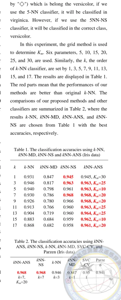
respectively. For a unclassified pattern (denoted by "◇") which is belong the versicolor, if we use the 5-NN classifier, it will be classified in virginica. However, if we use the 5NN-NS classifier, it will be classified in the correct class, versicolor.

In this experiment, the grid method is used to determine Km. Six parameters, 5, 10, 15, 20, 25, and 30, are used. Similarly, the k, the order of k-NN classifier, are set by 1, 3, 5, 7, 9, 11, 13, 15, and 17. The results are displayed in Table 1.

The red parts mean that the performances of our methods are better than original k-NN. The comparisons of our proposed methods and other classifiers are summarized in Table 2, where the results k-NN, kNN-MD, kNN-ANS, and kNN- NS are chosen from Table 1 with the best accuracies, respectively.

Table 1. The classification accuracies using k-NN, kNN-MD, kNN-NS and kNN-ANS (Iris data)

k k-NN kNN-MD kNN-NS kNN-ANS 1 0.931 0.847 0.945 0.945, Km=30 3 0.946 0.817 0.963 0.963, Km=25 5 0.940 0.798 0.961 0.963, Km=10 7 0.930 0.786 0.968 0.968, Km=20 9 0.926 0.780 0.966 0.968, Km=20 11 0.913 0.766 0.960 0.963, Km=25 13 0.904 0.719 0.960 0.964, Km=25 15 0.883 0.684 0.959 0.962, Km=10 17 0.868 0.682 0.958 0.961, Km=20

Table 2. The classification accuracies using kNN- ANS, kNN-NS, k-NN, kNN-MD, SVC-CV, and

Parzen (Iris data) kNN-ANS kNN-

NS k-NN kNN- MD

SVC -CV

Parze n 0.968

k=7, Km=20

0.968 k=7

0.946 k=3

0.847 k=1

0.95 1

0.941

(7)

Tables 1 and 2 show the following.

1. The results using modified metric are better than using the Euclidean distance and Mahalanobis distance.

2. For decreasing degree of accuracies, our methods outperform k-NN and kNN-MD when k is increasing.

3. In this case, the differences of kNN-ANS and kNN-NS are not remarkable.

4. Overall, kNN-ANS is a good and robust choice.

5.2. Heart Disease dataset

The University of California at Irvine maintains a repository of machine learning datasets, including a collection of data used for predicting the presence or absence of heart disease. The dataset we used is a cleaned version of the UCI Cleveland heart disease dataset, obtained from the University of Porto, in Portugal (Shervais and Zwick, 2003).

Figure 3. It represents the local region with respect to

"◇" of 5-NN and 5NN-NS, respectively. In the first panel, this region is a "sphere" with center " ◇ ."

However, this region is an "ellipsoid" with center "◇

" in the second panel.

The dataset contains 270 records, with 13 independent attributes, which have been extracted from a larger set of 75. These attributes include 5 continuous variables (A, D, E, H, J), one ordered variable (K), one integer (L), three binaries (B, F, I), and three multivalue nominal (E, C, M).

Table 3 displays the classification accuracies of Heart Disease dataset using 10- fold cross validation. It is obvious that the performance of kNN-ANS is the best. Although the result of the simple version kNN-NS does not outperform the results of kNN-MD and SVC-CV, it still has not bad performance.

Table 3. The classification accuracies using kNN- ANS, kNN-NS, k-NN, kNN-MD, SVC-CV, and

Parzen (Heart Disease dataset) kNN-

ANS

kNN-

NS k-NN kNN-

MD

SVC-

CV Parzen 0.848

k=7, K_m=100

0.826 k=7

0.674 k=7

0.833 k=7

0.844 0.674

(8)

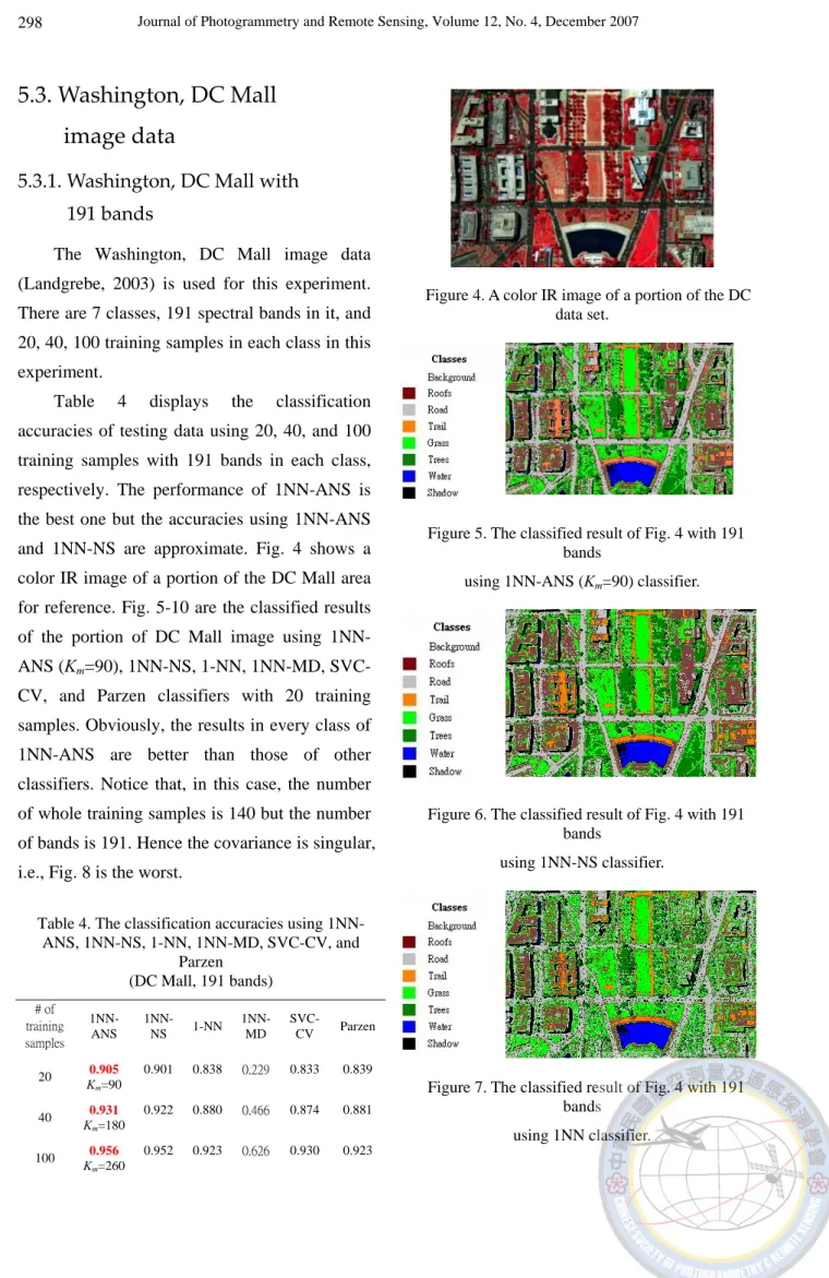
5.3. Washington, DC Mall image data

5.3.1. Washington, DC Mall with 191 bands

The Washington, DC Mall image data (Landgrebe, 2003) is used for this experiment.

There are 7 classes, 191 spectral bands in it, and 20, 40, 100 training samples in each class in this experiment.

Table 4 displays the classification accuracies of testing data using 20, 40, and 100 training samples with 191 bands in each class, respectively. The performance of 1NN-ANS is the best one but the accuracies using 1NN-ANS and 1NN-NS are approximate. Fig. 4 shows a color IR image of a portion of the DC Mall area for reference. Fig. 5-10 are the classified results of the portion of DC Mall image using 1NN- ANS (Km=90), 1NN-NS, 1-NN, 1NN-MD, SVC- CV, and Parzen classifiers with 20 training samples. Obviously, the results in every class of 1NN-ANS are better than those of other classifiers. Notice that, in this case, the number of whole training samples is 140 but the number of bands is 191. Hence the covariance is singular, i.e., Fig. 8 is the worst.

Table 4. The classification accuracies using 1NN- ANS, 1NN-NS, 1-NN, 1NN-MD, SVC-CV, and

Parzen (DC Mall, 191 bands)

# of training samples

1NN- ANS

1NN-

NS 1-NN 1NN- MD

SVC-

CV Parzen

20 0.905 Km=90

0.901 0.838 0.229 0.833 0.839

40 0.931 Km=180

0.922 0.880 0.466 0.874 0.881

100 0.956 Km=260

0.952 0.923 0.626 0.930 0.923

Figure 4. A color IR image of a portion of the DC data set.

Figure 5. The classified result of Fig. 4 with 191 bands

using 1NN-ANS (Km=90) classifier.

using 1NN-NS classifier.

using 1NN classifier.

(9)

using 1NN-MD classifier.

using SVC-CV classifier.

using Parzen classifier.

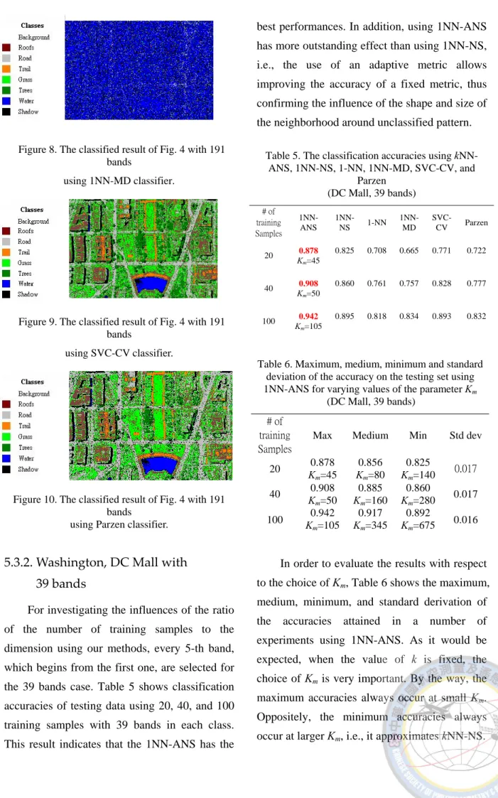
5.3.2. Washington, DC Mall with 39 bands

For investigating the influences of the ratio of the number of training samples to the dimension using our methods, every 5-th band, which begins from the first one, are selected for the 39 bands case. Table 5 shows classification accuracies of testing data using 20, 40, and 100 training samples with 39 bands in each class.

This result indicates that the 1NN-ANS has the

best performances. In addition, using 1NN-ANS has more outstanding effect than using 1NN-NS, i.e., the use of an adaptive metric allows improving the accuracy of a fixed metric, thus confirming the influence of the shape and size of the neighborhood around unclassified pattern.

Table 5. The classification accuracies using kNN- ANS, 1NN-NS, 1-NN, 1NN-MD, SVC-CV, and

Parzen (DC Mall, 39 bands)

# of training Samples

1NN- ANS

1NN-

NS 1-NN 1NN- MD

SVC-

CV Parzen

20 0.878

Km=45

0.825 0.708 0.665 0.771 0.722

40 0.908

Km=50

0.860 0.761 0.757 0.828 0.777

100 0.942 Km=105

0.895 0.818 0.834 0.893 0.832

Table 6. Maximum, medium, minimum and standard deviation of the accuracy on the testing set using 1NN-ANS for varying values of the parameter Km

(DC Mall, 39 bands)

# of training Samples

Max Medium Min Std dev

20 0.878 Km=45

0.856 Km=80

0.825

Km=140 0.017 40 0.908

Km=50

0.885 Km=160

0.860

Km=280 0.017 100 0.942

Km=105

0.917 Km=345

0.892

Km=675 0.016

In order to evaluate the results with respect to the choice of Km, Table 6 shows the maximum, medium, minimum, and standard derivation of the accuracies attained in a number of experiments using 1NN-ANS. As it would be expected, when the value of k is fixed, the choice of Km is very important. By the way, the maximum accuracies always occur at small Km. Oppositely, the minimum accuracies always occur at larger Km, i.e., it approximates kNN-NS.

(10)

Fig. 11-16 are the classification results of the portion of DC Mall image with 39 bands using 1NN-ANS (Km=45), 1NN-NS, 1-NN, 1NN-MD, SVC-CV, and Parzen classifiers with 20 training samples. Comparing Figure 11 and 12, we see that the performance of 1NN-ANS is similar to that of 1NN-NS, although the accuracy of 1NN-ANS is higher than that of 1NN-NS. Obviously, the results of 1NN-ANS and 1NN-NS are better than those of other classifiers.

Figure 11. The classified result of Fig. 4 with 39 bands using 1NN-ANS (Km=10) classifier.

Figure 12. The classified result of Fig. 4 with 39 bands using 1NN-NS classifier.

Figure 13. The classified result of Fig. 4 with 39 bands using 1-NN classifier.

Figure 14. The classified result of Fig. 4 with 39 bands using 1-NN-MD classifier.

Figure 15. The classified result of Fig. 4 with 39 bands using SVC-CV classifier.

Figure 16. The classified result of Fig. 4 with 39 bands using Parzen classifier.

6. Concluding Comments

In this paper we proposed a new approach using k-nearest neighbor classification scheme based on adaptive separability metric of NWFE (kNN-ANS) and its special case kNN-NS. Iris data, Heart Disease dataset, and real hyperspectral images show that the average classification accuracy of applying kNN-ANS is better than those of applying other classifiers.

Some findings are summarized in the following:

1. All performances of kNN-ANS are the best.

(11)

2. kNN-ANS and kNN-NS are more robust than traditional k-NN and kNN-MD.

3. The thematic maps of 1NN-ANS outperform those of other classifiers.

4. From above experiences, it is valid that using the adaptive separability of NWFE estimates an effective metric for computing a new neighborhood. The modified neighborhood shrinks in the direction with high separability and extends further in the other direction. Then the class conditional probabilities tend to be more homogeneous.

From the above findings, we may say that the use of kNN-ANS is more beneficial and yielding better results than other classifiers.

References

Baudat, G. and Anouar, F., 2000,

“Generalized discriminant analysis using a kernel approach,” Neural computation, 12(2000), pp.2385-2404.

Duin, R. P. W., 2002, “PRTools, a Matlab Toolbox for Pattern Recognition,”

[Online]. Available:

http://www.ph.tn.tudelft.nl/prtools/, Aug.

2002.

Fisher, R.A., 1936, “The use of multiple measurements in taxonomic problems,”

Annual Eugenics, 7, Part II, 179-188.

Friedman, J., 1994, “Flexible metric nearest neighbour classification,” Tech. Rep., Stanford University, November 1994.

Fukunaga, K., 1990, Introduction to Sataistical Pattern Recognition. San Diego, CA: Academic.

Hastie, T. and Tibshirani, R., 1996,

“Discriminant adaptive nearest neighbor classification,” IEEE Trans. on Pattern Analysis and Machine Intelligence, Vol.

18, No. 6, pp. 607-615.

Kuo, Bor-Chen and Landgrebe, David A., 2004, “Nonparametric weighted feature extraction for classification,” IEEE Trans. Geosci. Remote Sens., Vol. 42, No. 5, pp.1096-1105, May 2004.

Landgrebe, D. A., 2003, Signal Theory Methods in Multispectral Remote Sensing, John Wiley and Sons, Hoboken, NJ: Chichester.

Menahem Friedman and Abraham Kandel, 1999. Introduction to Pattern Recognition: Statistical, Structural, Neural, and Fuzzy Logic Approaches.

World Scientific, Singapore.

Shervais, S. and Zwick, M., 2003, “Using reconstructability analysis to select input variables for artificial neural networks,”

Proceedings of the International Joint Conference on Neural Networks, Vol. 4, pp. 3017-3021.

Short, R. and Fukanaga, K., 1980, “A new nearest neighbor distance measure,” in Proc. 5th IEEE Int. Conf. on Pattern Recognition, pp. 81-86.

(12)

以無參數的分散量為基礎的 k 最近鄰分類器

何省華

¹

李政軒

²

郭伯臣

³

摘要

k 最近鄰分類器是一個直覺且簡單的分類器。一個好的 k 最近鄰分類器期望類別的條件機率為局部一致。在本研究裡，我們使用 NWFE 的分散量建立一個有效的量測，進而找出新的鄰近區域。這個新的測量會將原來用歐式距離建立的鄰近區域延著分散量大的方向收縮且延著分散量小的擴張。而在修正後的鄰近區域的類別條件機率會趨向於更一致性。在實驗裡，k 最近鄰分類器使用修正後的鄰近區域會比原來的 k 最近鄰分類器及其它分類器分類效果好。因此，本文所提之方法可改善原始的 k 最近鄰分類器，而增進分類的效果。

關鍵詞: 樣式辨識、分類器、k 最近鄰分類器、nonparametric weighted feature extraction

收到日期:民國 96 年 09 月 14 日修改日期:民國 96 年 11 月 30 日接受日期:民國 96 年 12 月 03 日

1國立中興大學電機工程學系博士生

2國立交通大學電機與控制工程學系博士生

3國立台中教育大學教育測驗統計研究所教授