Capacity and Delay Tradeoffs of MotionCast with Base Stations

(1)

Capacity and Delay Tradeoffs of MotionCast with Base Stations

Luoyi Fu, Sen Yang, Xinbing Wang, Xiaoying Gan

Dept. of Electronic Engineering, Shanghai Jiaotong University, China Email: {fly, syang, xwang8, gxy}@sjtu.edu.cn

Abstract—In this paper, we study the multicast capacity-delay tradeoff of a wireless network consisting of mobile wireless nodes and base stations. m = n^b base stations are regularly placed in a square region and n is the number of mobile nodes in the network. We assume that mobile nodes move according to an independent and identical distributed (i.i.d.) pattern and each desires to send packets to k = n^d distinctive destinations. Under this basic network model, we study capacity, delay tradeoff in two transmission protocols: 2-hop relay algorithm with and without redundancy. We derive that the upper bound of per-node capacity of 2-hop relay algorithm without redundancy is O(n− min{1,1−b+d}) and its corresponding delay is Θ(nmin{1,1−b+d}). The lower bound of delay of this protocol is Θ(n¹^−b), with a smaller capacity O(n^b⁻²). For 2-hop relay algorithm with redundancy, the largest capacity and its corre- sponding delay are O(n− min{1,1−b+d}) and Θ(nmin{1,1−b+d}

2 ).

The smallest delay and its corresponding capacity are Θ(n^1−b² ) and O(n^b⁻³² ). When d > ¹₂ or b > min{^1+d₃ , 1− d}, adding base stations will improve the tradeoff mentioned in [7].

I. INTRODUCTION

Multicast is predominant in many practical situations due to its reduction of the total bandwidth. Li et al. in [4] studied the capacity of a large-scale random wireless network for multicast. As a generalization of the previous capacity bounds on unicast by Gupta and Kumar [5], they showed that the total multicast capacity is Θ(√

n

log n · ^√^W_k) when k = O(_{log n}ⁿ ), and Θ(W ) when k = Ω(_{log n}ⁿ ), where k is the number of destinations and W is the bandwidth of wireless channel.

Then, Li extended his research to a hybrid network consisting of static wireless nodes and base stations in [3]. Li et al.

compared the capacity of infrastructure mode and ad-hoc mode under static multicast model [2] and further extend the capacity study to three-dimensional space [11]. Capacity performance in sensor networks is analyzed by Liu et al. in [10].

All the results mentioned above are static cases. Different from them, Wang et al. [7] studied multicast for ad-hoc network through nodes’ mobility, defined as MotionCast, where nodes move according to an i.i.d. pattern and each packet has k distinctive destinations. They find that the per-node capacity and delay for 2-hop algorithm without redundancy (For each time-slot, if more than one nodes are performing as relays for a packet, they defined there is redundancy in the network.) are Θ(1/k) and Θ(n log k), respectively; and for 2-hop algorithm with redundancy they are Ω(1/k√

n log k) and Θ(√

n log k), respectively. Besides above, they first pointed out a tradeoff in multicast. Following that, they further investigate the tradeoff

of motioncast by adjusting the speed of mobile nodes [8].

More sophisticated technique such as MR-MC is adopted at the aim of capacity improvements in [9].

So far, intuitively, there still remains an open question: what are the capacity and delay if wireless nodes in hybrid networks have the ability to move? The key feature of this question is the combination of infrastructure and mobility. It means unlike static cases, packets are able to be sent to base stations via mobility, which may lead to a smaller delay. On the other hand, with the help of base stations, two mobile nodes in MotionCast model are easier to communicate. Hence, although the situation is more complicated than considering only one of them, a better capacity and delay tradeoff is expected.

To solve these problems, we investigate the per-node capacity, delay and their tradeoffs in a hybrid network. The hybrid network consists of two types of network terminals:

base stations and mobile wireless nodes. We assume that base stations are placed regularly in a square region and their transmission power is large enough to cover the whole region without overlapping. In addition, nodes are reshuffled at the beginning of each timeslot according to independent and identical distribution. The network model we raise is a generalized version of important models appeared before.

Removing the mobility, our model is reduced to Fang’s model in [2]. When the number of base stations is 0, it becomes Hu’s model in [7]. And if we set the number of destinations to a constant order after shutting down all the base stations, it turns to Neely’s unicast model in [1].

To start with, we propose a 2-hop relay algorithm without redundancy. This algorithm is a generalized version of the algorithm presented in [7]. The variation is that m base stations are included to help transmission. Thus, packets can be not only sent by ad-hoc mode, but also through base stations (Since the part of ad-hoc has been done in [7], we just consider the situation of transmission through base stations in this paper). A packet could be first cut and paste to another node or a base station before being delivered to destinations directly.

Next, we employ redundant packets transmissions to reduce the delay. In a 2-hop relay strategy with redundancy, a source first duplicates its packets till the number of duplications reaches a certain threshold before all the destinations receive the packet. Since packets have duplications, the probability that a certain packet meet its destinations or base stations increases, which may result in a smaller delay than that of 2-hop relay strategy without redundancy.

(2)

With the assumption that the number of base stations m = n^b and the number of destinations k = n^d. The main results of this paper are summarized as following: In 2-hop relay strategy without redundancy, the upper bound of capacity is Θ(¹_n) when k = Ω(m) and Θ(n^b^−d−1) when k = o(m), the corresponding delay are Θ(n) and Θ(n¹^−b+d) respectively.

The smallest delay is Θ(n¹^−b) while the capacity is O(n^b⁻²).

In these two cases, tradeoffs are _n¹2 and Θ(n^2b^−2d−2) respec- tively. When b > min{^1+d₂ ,²^−d₂ } or d = 1, it has a better tradeoff than using ad-hoc only. For 2-hop relay algorithm with redundancy, the largest capacity is Ω(¹_n) when k = Ω(m), Ω(n^b^−d−1) when k = o(m). The corresponding delay is Θ(√

n) and Θ(n^1−b+d² ) respectively. If we lower the capacity to O(n^b−3² ), we can obtain the smallest delay Θ(n^1−b² ). In addition, when d > ¹₂ or b > min{^1+d₃ , 1−d}, passing through base stations will improve the tradeoff mentioned in [7], which equals to _{kn log k}¹ . As to random walk mobility model, when we use 2-hop relay algorithm with redundancy, the delay is Θ(n^1+b² ) when k = Ω(m), and Θ(n¹^−b+2d² ) when k = o(m).

Other situations make small change to the results under i.i.d.

mobility model.

The rest of the paper is organized as follows. In next section, we establish the model that we are working on. In Section III, we calculate the tradeoff in 2-hop relay algorithm without redundancy while we study the one with redundancy in Section IV. In Section V, we discuss the results. Finally, we conclude in Section VI.

II. NETWORKMODEL

Cell Partitioned Network Model With Base Station: Suppose there are n mobile users randonly distributed in a square of length a. Then we divide this square into c non-overlapping cells with equal size as depicted. In order to avoid huge interference, we set the order of c is equal to the order of n. Thus, the node density q = n/c scales as Θ(1). We assume that nodes can send packets from one to another if both sender and receiver are in the same cell.

Then m = n^b(0≤ b ≤ 1) regularly distributed base stations divide the original region into m super cells. All these base stations are connected by wires so that they can communicate in Θ(1) delay. Every super cell containing one base station in the center includes c/m cells. A base station can communicate to any node in the same super cell while a node could only pass packet to base station when it is in the same cell with the base station.

Interference Model: We suppose uplink and downlink use different frequency to avoid interference. In a cell, only one node is allowed to transmit and only one node or a base station is allowed to receive. Users in neighboring cells are required to transmit over orthogonal frequency bands.

Mobility Model: Dividing time into constant duration slots, we adopt the i.i.d. mobility model. At the beginning of every time slot, all the n nodes are reshuffled so that they are randomly distributed in c cells with equal possibility. And, all these nodes are independent when choosing the cells to stay in the next time slot.

Traffic Pattern: We set the source-destination relationship before transmissions. Every node is an independent source corresponding to k destinations out of other n− 1 nodes.

Assume k = n^d(0≤ d ≤ 1). One source has to pass a packet to all the k destinations in order to make a successful pass. In addition, packets can be sent to a relay first and then transmit to destination through relay. And both mobile users and base stations can be regarded as relays. A mobile user relay can only send packet to one destination in one timeslot while a base station relay can send packet to many destinations in one timeslot.

Definition of Capacity: Assume packets arrive at node i with probability λi during each timeslot, i.e. as a Bernoulli process of arrival rate λipackets/slot. The maximum value of λ_i, which, in a certain schedule, can ensure every queue in nodes and base station will not accumulate to infinity as time goes to infinity, is called capacity of node i. For this model, because of symmetry, capacity of each node should be equal.

We denote it as λ and regard this value as the capacity of this network.

Definition of Delay: We define the expected time it takes a packet to reach all k destinations after it arrives the head of queue in source.

Definition of Redundancy: At each timeslot, if more than one nodes or base stations hold the same packet acting as a relay, we call this network “the network with redundancy”.

Otherwise it is “the network without redundancy”.

III. CAPACITY ANDDELAY IN THE2-HOPRELAY

ALGORITHMWITHOUTREDUNDANCY

In this section, we discuss the capacity and delay when packets are sent all by infrastructure in the same condition.

A. Upper bound of capacity

In this subsection, we calculate the upper bound of the capacity and it corresponding delay. Here we must note that in this paper although we state the specific algorithms before we analyze the bounds of capacity and delay, them are not algorithm-dependent and can be applied to any other algorithms.

Under the conditions mentioned above, we consider the following scheme:

2-hop Relay Algorithm Without Redundancy - capacity : During each timeslot, in each cell containing a base station, a node is chosen as a source to base station uniformly randomly. If this node has a new packet to transport, it sends this packet to the base station in the cell. If not, remain idle.

1) When k = ω(m): First, we consider the situation that the number of destinations is much larger than that of base stations, i.e. 0 ≤ b < d ≤ 1. Under this condition, we have the following lemma.

Lemma 1: In each super cell, there are at most ^3k_m nodes w.h.p., where k = n^d, the number of destinations, m = n^b, the number of base stations, and b < d.

Proof: One can refer to [6] for the proof.

(3)

As we know, one base station can only send one packet in one timeslot. For any packet, due to Lemma 1, there are at most ^3k_m destinations which can be reached by a base station.

In the other words, in one timeslot, one base station, w.h.p., can make ^3k_m significant transmission at most.

Each base station has a queue to store the packets to be sent. Assume the input rate is λ_i and output rate is µ_i. Then the number of packets arriving at m base stations in an interval [0, T ] is λiT m. To make a successful pass, a packet has to be sent k times at least, which leads to the fact that the total number of transmissions is λiT mk. As mentioned above, for a certain packet, one base station can at most make ^3k_m significant transmissions in one timeslot. We have the following equation:

λiT mk≤ 3k

mT m (1)

i.e., λi ≤ _m³. As a result, the upper bound of input rate of each queue in base station is Θ(_m¹).

As mentioned before, base stations can pass packets in one hop if destinations are in its transmission range, which will lead to a constant order time cost. Thus, the waiting time in the queue of source contributes the main part of delay. There are m base stations distributed in c cells. Thus, every timeslot, the probability that a node could meet a base station is ^m_c. Since the input rate of each queue in base station is Θ(_m¹), the probability that a given packet is sent from source-node to a base station can be calculate as following: P ≤ Θ(^m_c×_m¹)×¹_q, q is the density of nodes in network. Recall that m = n^b and c = Θ(n), P ≤ Θ(¹_n). Thus, delay of 2-hop Relay Algorithm Without Redundancy is D = 1/P ≥ Θ(n).

Since input rate of each queue in base stations is Θ(_m¹), during time interval [0, T ], the total number of packets sent to base stations is Θ(_m¹)× T m. To guarantee a stable network, the throughput of whole network cannot exceed the packets that base stations are able to serve in time interval [0, T ]. We have:

λT n≤ Θ(1

m)× T m (2)

i.e., λ ≤ Θ(¹_n). Therefore, the upper bound of capacity in 2-hop Relay Algorithm Without Redundancy is Θ(_n¹).

2) When k = Θ(m): When k = Θ(m), i.e. b = d, we will show the situation is quite similar to k = ω(m) by the following Lemma.

Lemma 2: When the number of base stations and the num- ber of destinations are in the same order, n^b, and destinations are uniformly distributed into m supercell, the number of base stations which contain at least one destination, denoted as v = n^t w.h.p., is order n^b.

Proof: Consider the probability that all k destinations are in n^t supercells, where 0 ≤ t < b ≤ 1. This probability consists two parts. One is randomly choosing n^t supercells out of n^b ones. The other is all k destinations are in these chosen supercells. By combining these two parts, we get the

probability:

P = C_nⁿb^t× (n^t

n^b)ⁿ^b < n^bn^t^−(t−b)n^b

Since 0 ≤ t < b ≤ 1, P → 0 when n → ∞. Thus, w.h.p., t = b, i.e. the number of base stations which contain at least one destination, w.h.p., is order n^b.

Due to Lemma 2, ^m_v = Θ(1), which leads to the fact that during one timeslot, m base stations, w.h.p., can only finish constant order transmissions of packets. Thus, the output rate of the waiting queue in one base station is Θ(_m¹).Similarly, when k = ω(m), we get λ = Θ(_n¹) and D = Θ(n).

To sum up, we have the following theorem:

Theorem 1: Under 2-hop without redundancy scheme, us- ing infrastructure mode only, if k = Ω(m), i.e. d ≥ b, the capacity and delay of network are ¹_n, n, respectively. And the tradeoff is λ/D = _n¹2.

3) When k = o(m): Clearly, when k = o(m), the expectation of the number of supercells which contain at least one destination isE(v) = k, w.h.p. from Lemma 3.

Lemma 3: When k = o(m) and m→ ∞, for any supercell S_i which contains at least one destination, S_icontains exactly one destination with high probability.

Assume ε = b− d − δ > 0, where δ is a tiny positive constant. Then k× n^ε = n^b^−δ = o(n^b) = o(m). Applying Lemma 3, these kn^ε destinations, w.h.p., are distributed in kn^ε different supercells and every supercell only contain one destination. Thus, at least, kn^εdestinations can receive packets from base stations in one timeslot simply by the scheme that one base station passes a packet to one destination in the same supercell. As a result, during one timeslot, the whole network can make at least n^ε successful passes. The output rate of the queue in each base station is ⁿ_n^ε_b = n^−d−δ. Similar to the first two situation, The probability that a given packet is sent from source-node to a base station is P = Θ(^m_c × n^−d−δ)×

1

q = Θ(n^ε), q is the density of nodes in network, which is in a constant order. And capacity λ = Θ(n^ε⁻¹) and delay D = Θ(n¹^−ε). Because δ can be any tiny positive constant, ε can be quiet close to b− d, ε → b − d. Therefore, we have the following theorem:

Theorem 2: Under 2-hop without redundancy scheme, us- ing infrastructure mode only, if k = o(m), i.e. d < b, the capacity and delay of network are Θ(n^b^−d−1), Θ(n¹^−b+d), respectively. And the tradeoff is λ/D = Θ(n^2b^−2d−2).

B. Lower bound of delay

The result we get above has a large capacity. But in some applications such as voice transmission, we consider more on delay rather than capacity. In this subsection will show another algorithm which sacrifices capacity to improve delay.

2-hop Relay Algorithm Without Redundancy - delay : Re- gard all n queues in n nodes as one big queue. All the packets arrived in each queue are sent one by one, which means every time slot there is only one packet transmitting in the network.

The order is determined by the rule first comes, first sends.

(4)

If two packets arrive in different nodes in the same time slot, choose the packet from the session i which maximizes (tp+ i) mod n to be sent first, others wait in the queue. The chosen one is sent by the following: when the node and one of base stations are in the same cell. The node sends the packet to the base station and the base station transmit it to all the destinations. Else, remain idle.

The above protocol is ‘fair’ in that in case of ties, session i packets are given top priority every n timeslots. First, let TN

denote that when a new packet reaches the head of the line at its source queue, the time required for the packet to reach its destination. The probability that a certain node meets a base station is ^m_n. Thus, the expectation of time that a packets is sent to a base station is _mⁿ. That means, TN =_mⁿ.

Then we use the following lemma to calculate the delay and capacity.

Lemma 4: Suppose inputs to a single server queue are Poisson with memoryless service times that are independently bounded in expectation by a value TN. If the arrival rate is λ, where λ < 1/TN, then average delay satisfies:

D≤ 1 2+ TN

1− ρ (3)

where ρ , λTN. The expression on the right hand side of the above inequality is the standard expression for delay in an M/M/1 queue with i.i.d. service times TN that are restricted to start on slot boundaries.

The proof of this lemma is from [1]. According to Lemma 4, we have:

Theorem 3: For Poisson inputs with rates λifor each source i, the network under the protocol is stable whenever Σiλi<

1/TN, with average end-to-end delay satisfying:

D≤ 1 2+ TN

1− ρ (4)

where ρ , ΣiλiTN. Note that TN = _mⁿ. Thus, when all sources have identical input rates λ, stability and logarithmic delay is achieved when λ = O(_n^m2).

Given that m = n^b, the tradeoff between capacity and delay is λ/D = O(n^2b⁻³).

Applying 2-hop Relay Algorithm Without Redundancy - de- lay, delay is able to achieve the same order as TN. Obviously, there are no methods or algorithms that could obtain a delay smaller than TN, which is the number of timeslots spent on passing a single packet in network. Thus, we could conclude that the lower bound of delay is n¹^−b with the capacity λ = n^b⁻².

IV. CAPACITY ANDDELAY IN THE2-HOPRELAY

ALGORITHMWITHREDUNDANCY

In this section, we will discuss the situation in the 2-hop relay algorithm with redundancy. Just like the part without redundancy, we compute the largest capacity and smallest delay respectively.

A. Upper bound of capacity

In this subsection, we calculate the upper bound of capacity.

In order to obtain maximum capacity, the relationship between the number of destinations, k and the number of base stations, m is taken into account.

1) When k = Ω(m): We change the 2-hop Relay Algorithm Without Redundancy - capacity by duplicate packet first before capture. Noticing that all base stations in network can still only make constant order successful passes in one timeslot, which is the same as the strategy without redundancy, we conclude that the upper bound of per-node capacity is also _n¹. The following algorithm achieves this upper bound.

2-hop Relay Algorithm With Redundancy - capacity I: Di- vide timeslot into two parts. One is odd, and the other is even.

During every odd timeslot, we do the following things:

Source-to-Relay Transmission: The sender transmits packet SN , and does so upon every transmission opportunity until

√n duplicates have been delivered to distinct relay nodes (possible be some of the destinations), or until the k destina- tions have entirely obtained SN . After such a time, the sender number is incremented to SN + 1. If the sender does not have a new packet to send, stay idle.

Relay-to-Destination Transmission: When a node is sched- uled to transmit a relay packet to its destinations, the following handshake is taking place:

• The receiver delivers its current RN number for the packet it desires.

• The transmitter sends packet RN to the receiver. If the transmitter does not have the requested packet RN , it stays idle for that slot.

• If all k destinations have already received RN , the transmitter will delete the packet which has SN number equal to RN in its buffer.

During every even timeslot, we do the following things:

In each cell containing a base station, a node is chosen as a source to base station uniformly randomly. If this node has at least a packet to transport, it randomly picks one packet and sends this packet to the base station in the cell. If not, remain idle.

Next, we demonstrate the performance of this scheme by providing theorem 4.

Theorem 4: When k = Ω(m), 2-hop Relay Algorithm With Redundancy scheme can achieve Θ(√

n) delay bound with the capacity in order O(_n¹).

2) When k = o(m): Since the number of successful passes that all base stations in network are able to make in one timeslot remains same although we apply redundancy to help transmission, the upper bound of capacity is still O(n^b^−d−1).

The scheme when k = o(m) is quite similar to that when k = Ω(m), with a little change on the number of duplications to n^1−b+d² . Due to page limitations, we put the detailed algorithm to our technical report [6].

Using similar techniques, we can obtain the delay TN = Θ

( n^1−b²

)

. And the following lemma shows the delay.

(5)

Tradeoff

k 2

2 d b −

=

) / 1

( n

Θ )

/ 1 ( n² Θ

) / (m² n³ Θ

) / 1 ( n Θ

) (m

Θ Θ(n)

2 b 1 d+

= )

/ (m² n² Θ

upper capacity

lower D reference

curve in [2]

) 1 ( Θ

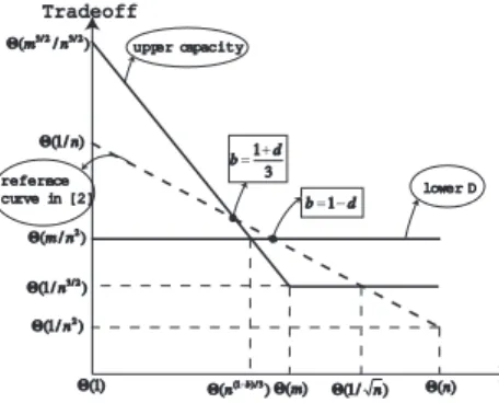
Fig. 1: Tradeoff against destinations in 2-hop w.o. redundancy

Theorem 5: For Poisson inputs with rates λifor each source i, the network under the protocol is stable whenever Σiλ_i<

1/T_N, with average end-to-end delay satisfying: D≤ ¹₂+₁^T_−ρ^N , where ρ, ΣiλiTN.

Note that T_N = Θ(n^1−b² ). Thus, when all sources have identical input rates λ, stability and logarithmic delay is achieved when λ = O(n^b−3² ). The tradeoff between capacity and delay is λ/D = O(n^b⁻²). The lower bound of delay is n^1−b² with the capacity λ = n^b−3² .

V. DISCUSSION

It can be seen from our results that applying redundancy reduces delay and due to base stations, without an expense of the capacity. The ratio between per-node capacity and delay for these two protocols are O(n−2 min{1,1−b+d}) and Θ(n⁻3 min{1,1−b+d}

2 ), respectively. Redundancy provides a better tradeoff. Moreover, if we expect to obtain their lower bound of delay, we see that redundancy improves both per- node capacity and delay. By using redundancy, the tradeoff increases to n^b⁻² from n^2b⁻³.

Further more, compared with the motioncast capacity-delay tradeoffs of ad-hoc mode developed in [7], we find that tradeoff of the 2-hop relay algorithm without redundancy is better when b > min{^1+d₂ ,²^−d₂ } or d = 1. Figure 1 shows the tradeoff against the number of destinations, k. The line achieving the upper bound of capacity declines as the number of destinations increases until k = Θ(m), and then it remains Θ(_n¹₂). Meanwhile, the line achieving the lower bound of delay is horizontal, which means the capacity and delay tradeoff has nothing to do with the number of destinations.

When it comes to 2-hop relay algorithm with redundancy, combination of infrastructure and mobility also helps transmission. The tradeoff is shown in Figure 2. The trend of tradeoff-destination line in Figure 2 is similar to Figure 1, but the tradeoff is larger with the same number of destinations. In comparison with the results in [7], transmission through base stations will be a better choice when d > ¹₂ or b > min{^1+d₃ , 1− d} than using ad-hoc in [7].

VI. CONCLUSION

This paper studies capacity and delay tradeoffs of Motion- Cast using infrastructure. We present the performance of the

Tradeoff

k )

/ 1 ( n³^/² Θ

) / 1 ( n² Θ

) / (m³^/²n³^/² Θ

) / 1 ( n Θ

) / (mn² Θ

) (n⁽¹⁺^b⁾^/³

Θ Θ(m) Θ(1/ n) Θ(n) )

1 ( Θ

3 b 1 d+

=

d b= 1− upper capacity

lower D reference

curve in [2]

Fig. 2: Tradeoff against destinations in 2-hop w. redundancy

2-hop relay algorithm without redundancy and then utilize redundancy to improve the tradeoff largely. After that, we consider random walk mobility instead of i.i.d. mobility. By comparing with the results in ad-hoc mode under i.i.d. mobility, we found that in 2-hop relay algorithm without redundancy scheme, with some conditions satisfied, using infrastructure mode is better than ad-hoc mode. And in 2-hop relay algorithm with redundancy scheme, in some specific conditions, using infrastructure mode is better than ad-hoc mode.

VII. ACKNOWLEDGMENT

This work is supported by National Basic research grant (2010CB731803), NSF China (No. 60832005,60972050);

China Min- istry of Education Fok Ying Tung Fund (No.122002); Qual- comm Research Grant; National Key Project of China (2009ZX03003-006-03, 2010ZX03003-001- 01, 2010ZX03002-007-01).

REFERENCES

[1] M. J. Neely and E. Modiano, “Capacity and delay tradeoffs for ad hoc mobile networks,” IEEE Trans. Inform.Theory, vol. 51, no. 6, pp. 1917- 1937, June 2005.

[2] P. Li and Y. Fang, “Impacts of Topology and Traffic Pattern on Capacity of Hybrid Wireless Networks,” IEEE Trans. Mobile Computing, vol. 8, no. 12, pp. 1585-1595, Dec. 2009.

[3] X. Mao, X. Li and S. Tang, “Multicast Capacity for Hybrid Wireless Networks,” in Proc. ACM MobiHoc, May 2008.

[4] X. Li, S. Tang, O. Frieder, “Multicast Capacity for Large Scale Wireless Ad Hoc Networks,” in Proc. ACM MobiCom, Sept. 2007.

[5] P. Gupta and P. R. Kumar, “The capacity of wireless networks,” IEEE Trans. Inform. Theory, vol. 46, no. 2, pp. 388-404, Mar. 2000.

[6] L. Fu, S. Yang, X. Wang, X. Gan, “Capacity Delay Tradeoff of Motioncast with Base Station,” [Online], technical report. Available at http://iwct.sjtu.edu.cn/Personal/xwang8/paper/MotioncastBS.pdf [7] X. Wang, W. Huang, S. Wang, J. Zhang and C. Hu, “Delay and Capacity

Tradeoff Analysis for MotionCast,” in IEEE/ACM Trans. Networking, No. 99, 2011. DOI:10.1109/TNET.2011.2109042.

[8] X. Wang, Y. Bei, Q. Peng and L. Fu, “Speed Improves Delay-Capacity Tradeoff in MotionCast,” in IEEE Trans. Parallel and Distributed Systems, No. 99, pp:729 - 742, 2011. DOI: 10.1109/TPDS.2010.126.

[9] H. Li, Y. Cheng, C. Zhou and P. Wan, “Multi-dimensional conflict graph based computing for optimal capacity in MR-MC wireless networks”, in Proc. IEEE ICDCS, Genoa, Italy, Jun. 2010.

[10] Y. Liu, Y. He, M. Li, J. Wang, K. Liu, L. Mo, W. Dong, Z. Yang, M. Xi, J. Zhao and X. Li, “Does Wireless Sensor Network Scale?

A Measurement Study on GreenOrbs”, in IEEE INFOCOM 2011, Shanghai, China, Apr. 2011.

[11] P. Li, M. Pan and Y. Fang, “The Capacity of Three-Dimensional Wireless Ad Hoc Networks”, in IEEE INFOCOM’11, Shanghai, China, Apr.

2011.