Predicting Protein Subcellular Location Using Hybrid Approach
Shih-Hao Chen, Han-Wen Hsiao*, Wen-Hung Hsiao
Institute of Bioinformatics, Taichung Healthcare and Management University
*E-mail: [email protected]
摘要
蛋白質功能與其在細胞中的胞器位置非常相關,因 此藉由預測蛋白質在細胞中的位置可瞭解蛋白質功 能,特別是許多生物都已被定序出來,需要有效的 方法快速且大量地分析序列。文獻中已有不少相關研 究,但結果仍有改善空間。本文提出一套混合的方法 結合數種特徵向量對 17655 條蛋白質進行分析,其 總精確度可達到 91.5%。
關鍵字:胞器位置、蛋白質功能預測 Abstract
Biologically, the function of a protein is highly related to its subcellular localization. It is necessary to develop a reliable method for protein subcellular localization pre- diction, especially when large-scale genome sequences are to be analyzed. Various methods have been proposed to perform the task. The results, however, are not satis- factory in terms of effectiveness and efficiency. A hybrid approach using naïve Bayesian classifier with informa- tion gain ratio and k-nearest neighbor classifier is pre- sented. The total accuracy for a set of 17655 proteins can reach up to 91.5%.
Keywords: subcellular localization, function prediction Introduction
According to the central dogma of molecular biology, a eukaryotic DNA sequence is transcribed to an RNA se- quence, and then translated to a protein, which can be addressed for different target organelles or compartment, depending on its function [12]. Conventionally, three techniques are necessary to identify the subcellular local- ization of a protein [24]: cell fractionation, electron and fluorescence microscopy images. Kumar et al. [20], for example, determined the subcellular localization of 2744 yeast proteins by immunolocalization of tagged gene products. However, wet lab experiments are usually time-consuming and not cost-effective. It is possible to alleviate these problems and reduce the time span of re- search by using in silico approaches to perform predic- tion tasks prior to conducting laboratory experiments.
Nakai and Kanehisa [26, 27] were the first to predict protein localization sites systematically, and the results were helpful to the biologists. Later, numerous works re- garding subcellular localization prediction for protein function analysis have been reported in the literature [8, 10, 11, 14]. In general, these works can be reviewed from two perspectives: feature representation and classi- fication approach.
It is known that the subcellular localization of a protein is determined by sorting signal [1] of around 15 to 60 amino acid residues at the N-terminal. It was found out that positively charged amino acid residues tend to con- gregate at the front part of the signal peptide, hydropho-
bic at the middle, and polar at the rear [33]. Another dis- covery is that Ser and Thr are frequent in chloroplast tar- geting peptides, while the negatively charged amino acid residues, like Asp and Glu, are less [34]. Consequently, recognizing sorting signal as a feature of protein is meaningful [13, 25]. A serious problem of using sorting signal is that protein sequences from draft genomes are usually incomplete and lack of signal peptides [21].
Amino acid composition is the simplest feature by calcu- lating the frequencies of 20 kinds of amino acid residues [17, 29, 30]. It has a very high coverage but is not char- acteristic [17]. Dipeptide composition [28] is a variation that the frequencies of 202 combinations of two adjacent amino acid residues form a vector in a feature space of 400 dimensions. Different features may be extracted by a generalized autocorrelation function of the physicochem- ical properties, such as hydrophobicity and polarity, along an amino acid sequence [5, 6, 7]. Recently, func- tional domain composition [4, 9] has been utilized popu- larly due to its representative characteristics that proteins having particular domains often localize to specific or- ganelles [23].
Various algorithms have been applied to the problem of protein subcellular localization prediction. Reinhardt and Hubbard [29] used amino acid composition in combina- tion with neural network approach to predict subcellular localization of prokaryotic and eukaryotic proteins. The total accuracies achieved 81% for 3 subcellular locations in prokaryotic organisms and 66% for 4 locations in eu- karyotic organisms. Yuan [35] adopted Markov chain models to achieve better accuracies of 89% and 73% for prokaryotic and eukaryotic sequences on the same data set. Lately, support vector machines (SVM) introduced by Vapnik [32] have been gaining popularity in the aca- demic areas due to many attractive features for super- vised classification and regression. Hua and Sun [17]
proposed a method using amino acid composition and SVM to work on the same data set. The total prediction accuracies reached 91.4% for 3 subcellular locations in prokaryotic organisms and 79.4% for 4 locations in eu- karyotic organisms. Different from the previous cases, Chou and Cai [9] used functional domain composition and SVM for subcellular localization prediction. Later, Cai et al. [4] applied the same approach to predict mem- brane protein types by supervised classification per- formed in a hyperspace with dimensions up to 2005, and reached an overall accuracy up to 87.3%. Instead of us- ing functional domain composition, Mott et al. [23]
turned their attention to the co-occurrence of pairs of do- mains extracted from the SMART domain databank [31].
The co-occurrence matrix was then projected to a two- dimensional Euclidean space by multidimensional scal- ing, and thus the domains scattered as clusters of dots over this space. A number of Gaussian kernels as proba-
bility functions were applied to fit to the clusters. Fi- nally, the subcellular location of a protein was deter- mined by its domains locating on which Gaussian hills of the landscape and each hill represented a specific subcel- lular location. Their approach achieved an accuracy of 92% but was inefficient. Huang and Li [18] utilized dipeptide composition and fuzzy k-nearest neighborhood method to achieve an overall accuracy about 80% in a jackknife test. Cai and Chou [8] used both functional do- main composition and pseudo-amino acid composition as features to perform prediction separately by using the nearest neighborhood method. The result of using pseudo-amino acid composition as feature, however, was a supplement only when proteins without (known) func- tional domain.
In this paper, a considerably straightforward yet greatly effective approach based on weighted naïve Bayesian classifier and nearest neighborhood method is presented.
Three commonly used features are considered as protein sequence descriptors, i.e. functional domain, amino acid composition, and dipeptide amino acid composition. The paper is organized as follows. The following section de- scribes the datasets and the proposed methods, including the evaluation method. The experimental results as well as discussion are provided subsequently. The final sec- tion concludes the study.
Materials and Methods
In this study, three different datasets of eukaryotic pro- teins shown in Table 1 were all generated from the SWISSPROT database [2]. The first dataset D1 was gen- erated by Park and Kanehisa [28] from release 33.0; the second dataset D2 was generated by Chou and Elrod [10]
from release 35.0 and later used by Chou and Cai [9].
We generated the third dataset D3 from release 42.0. Ac- cording to the protein’s subcellular localization, each dataset was divided into twelve categories: chloroplast, cytoplasm, cytoskeleton, nucleus, extracellular, endo- plasmic reticulum, Golgi apparatus, lysosome, plasma membrane, peroxisome, mitochondria, and vacuole.
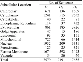
Table 1. The number of protein sequences within each subcellular localization category.
Subcellular Location No. of Sequence
D1 D2 D3
Chloroplast 671 136 1609
Cytoplasmic 1241 515 2632
Cytoskeletal 40 22 81
Endoplasmic Reticulum 114 37 432
Extracellular 861 185 3926
Golgi Apparatus 47 15 186
Lysosomal 93 35 151
Mitochondrial 727 66 1414
Nuclear 1932 209 3331
Peroxisomal 125 25 321
Plasma Membrane 1674 592 3493
Vacuole 54 20 79
Total 7579 2191 17655
Notice that proteins in dataset D2 were elaborately se- lected by the following five criteria [9, 10]. However, only the first three criteria were applied to D1 and D3: 1. Sequences annotated as fragments were not selected;
2. Sequences contained ambiguous amino acids were not considered;
3. Sequences annotated multiple subcellular locations were filtered out;
4. Sequences without clear annotation were removed;
and
5. Only one sequence was selected from a number of proteins with identical name but from different species.
Moreover, three sequence descriptors were considered in this study: amino acid composition, dipeptide amino acid composition, and functional domain composition. To re- trieve the functional domains of each protein from the Conserved Domain Database (cdd v1.65), the Reverse Position Specific BLAST (RPS-BLAST 2.2.6) was used with E value set as 10-2.
In this study, three frequently used features were consid- ered for sequence classification to predict the subcellular localization of proteins: functional domain composition, amino acid composition, and dipeptide amino acid com- position. However, the integrated feature vector could be up to thousands of dimensions and difficult for classifi- cation. The naïve Bayesian classifier was adopted in the first phase of classification task due to its demonstrated performance in many areas [15]. Suppose that a protein is expressed as a set of attributes a1, a2, ... , an with an annotated subcellular location s S, where S is a finite set of ns subcellular locations. The Bayesian approach to classifying the subcellular localization of a new protein, giving its attributes, is to maximize a posterior hypothe- sis of assigning the most probable sMAP to the protein.
) ( )
| , , , ( max arg
) , , , (
) ( )
| , , , max ( arg
) , , ,
| ( max arg
2 1
2 1 2 1
2 1
j j S n
s
n j j n S
s
n S j
MAP s
s P s a a a P
a a a P
s P s a a a P
a a a s P s
j j j
(1)
where j = 1 ... ns and P(a1, a2, ... , an) is a constant that can be disregarded. The two terms in the above equation can be estimated from the training dataset. Estimating P(sj) is straightforward, while the P(a1, a2, ... , an | sj) term is not that simple. An assumption to simplify the computation is that the attributes are conditionally inde- pendent, which can yield a result of replacing the first term by the product of the conditional probability for the individual attributes, i.e.
n
i
j i S j
NB s P s P a s
s
j 1
)
| ( ) ( max
arg (2)
where sNB means the output of naïve Bayesian classifier.
In the case of binary attributes ai representing functional domain composition, P(ai | sj) is basically the portion of proteins belonging to subcellular location sj. For numeric attributes ai describing dipeptide amino acid composition and amino acid composition, P(ai | sj) is calculated from a Gaussian density function of ai
2 2
2 ) exp (
2 1
) , , ( )
| (
ij ij i ij
ij ij i j i
a a
g s a P
(3)
where ij and ij are the mean and standard deviation of attribute ai of training samples belonging to subcellular localization sj. Preferably, the values for comparison are normalized within a finite range. In reality, one protein could be represented by thousands of attributes, and thus the product of n probabilities would result in a numerical problem. In order to remedy this problem, Equation 2 is modified as follows:
/ )
| ( log )
( log exp
) ( max arg
1 n i
j i j
j
S j NB s
s a P s
P p
p s
j
(4)
where 0 < pj < 1 and is a regulatory parameter.
One rational assumption is that some attributes ai may be strongly associated with a specific subcellular location sj. Instead of treating each attribute as equally important, a weighted version of Equation 4 is presented as
/ )
| ( log )
( log exp
) ( max arg
1 n i
j i i
j j
S j NB s
s a P w s
P p
p s
j
(5)
where the weights wi should be self-decided by the dataset. Numerous attribute selection techniques have been reviewed in the literature [16]. The information gain ratio is considered for its simplicity. First, the infor- mation or entropy of np proteins relative to classification of ns subcellular locations is defined as
ns
j
j
j P s
s P E
1
) ( log )
( (6)
After partitioning the set of proteins in accordance with no outcomes of an attribute ai, the expected information can be acquired as the weighted sum of entropies over the subsets
o ns
j j k j k
n
k k
i P o P s o P s o
a E
1 1
)
| ( log )
| ( ) ( )
(
(7)
where ok is one of no outcomes of attribute ai and P(ok) is the portion of proteins having outcome ok in attribute ai. For binary attributes ai, it is rather simple to get P(sj | ok) by counting the number of proteins at subcellular loca- tion sj under the condition of outcome ok. Data sets with numeric attributes should be converted to discrete values prior to information calculation. A simple conversion of ai to oi is defined as
0 otherwise ) (
if
1 i ij ij
i
o a
(8) where ij and ij are mentioned previously. The informa- tion gain with respect to attribute ai is
) ( )
(ai E E ai
Gain (9)
The information gain is further normalized by the split information to obtain the gain ratio. The larger the gain ratio value is, the more important the attribute is.
) ( log ) ( )
(
) (
) ) (
(
1
k n
k
k i
i i i
o P o
P a
SplitInfo
a SplitInfo
a a Gain
GainRatio
o
(10)
The result of naïve Bayesian classifier with information gain ratio is considered as the input for the second phase of classification. The dimensionality of input vector can still be up to hundreds of dimensions. Thus, the k-nearest neighborhood method is adopted for its effectiveness and simplicity. The nearest neighbors of an instance in such a space n are defined in terms of the Euclidean distance
n
k
j k i k j
i x a x a x
x d
1
)2
( ) ( )
,
( (11)
To compare with other works, the experimental results were evaluated by the same testing procedures [17, 28].
Let N be the total number of protein sequences in a dataset and S be the category number of subcellular lo- calizations, i.e. S = 12 in this study. Moreover, TPi, TNi, FPi, and FNi are defined as the numbers of true positive, true negative, false positive, and false negative se- quences of location i, respectively. Accordingly, the in- dividual accuracy (IA), location accuracy (LA), total ac- curacy (TA), and Matthew’s Correlation Coefficient (MCC) [22] are defined as follows:
N TP TA
S IA LA
FP TN FN TN FP TP FN TP
FN FP TN MCC TP
FP TP IA TP
S i
i S i
i
i i i i i i i i
i i i i i
i i
i i
1 1
) )(
)(
)(
(
where i = 1 ... S. It is clear from the definition of MCC that a completely correct classification yields a result of one.
Results and Discussion
In this study, amino acid composition, dipeptide amino acid composition, and functional domain composition were utilized to form a feature vector. After extracting domains from each protein by RPS-BLAST 2.2.6, the
datasets D1, D2, and D3 contained 3824, 2968, and 8418 different conserved domains, respectively. The amino acid composition and dipeptide amino acid composition of each protein also formed a vector of 20+400 dimen- sions. The final vector dimensionality describing each protein in dataset D1, for example, was 3824+20+400.
Each dataset was classified by weighted naïve Bayesian classifier with information gain ratio. The result for each protein was in fact a vector of probabilities with respect to twelve subcellular locations. This vector was then re- combined with the 420-dimensional vector obtained pre- viously to form a vector of 432 dimensions. Finally, all proteins representing by a 432-dimensional vector were classified by the k-nearest neighborhood method, where k = 3 was the optimal number to achieve the best result.
The procedure is illustrates in Figure 1.
Figure 1. Flow chart for predicting subcellular location.
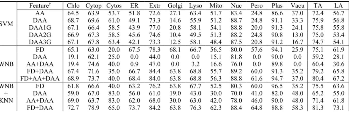
The SVM part of Table 2 replicates the prediction results by Park and Kanehisa [28], where the task was done by RBF-kernel SVM and evaluated by 5-fold cross valida- tion. The features they used were amino acid composi- tion, dipeptide amino acid composition with 0, 1, 2, and 3 gaps. Their dataset was adopted as dataset D1 for per- formance comparison. The approaches were weighted naïve Bayesian classifier without and/or with k-nearest neighborhood method or with learning vector quantiza- tion, denoted as WNB, WNB+KNN, and WNB+LVQ, respectively.
The results about actual and predicted classification of dataset D1 by WNB+KNN using those three composi- tions as features can be presented as a confusion matrix [19] in Table 3. As shown in Tables 2 and 3, it is inter- esting that the classes of plasma membrane, extracellu- lar, and nucleus have a very high accuracy. On the con- trary, proteins belong to the categories of chloroplast, mitochondrial, and nuclear tend to be predicted incor- rectly as that of cytoplasmic, and vice versa. Further- more, vacuolar, cytoskeleton, peroxisomal, Golgi, endo- plasmic reticulum, and lysosomal classes contain very few protein sequences and have unreliable and inaccu- rate result. The phenomena may be due to the proteins involved in a secretory pathway or driven by protein in- teractions.
Another comparison was made in Table 4 that the pre- diction accuracies were evaluated using 5-fold cross val- idation test for both datasets 1 and 2. Owing to the changes of code naming, very few proteins in the origi- nal datasets could not be found. In the second dataset,
Chou and Cai [9] performed the classification task by SVM using functional domain composition as the input feature for each protein and reached a total accuracy of 75%. The proposed hybrid approach combining three compositions could achieve better total accuracies of 82% and 79% for D1 and D2, respectively, especially for those classes containing fewer proteins.
The same feature and approach were applied to the dataset D3, where valid sequences were arbitrarily se- lected as many as possible from the SWISSPROT data- bank. The predicted results shown in Table 5 were evalu- ated by the 5-fold cross-validation test as well. Interest- ingly, the total accuracy of the set of 17655 proteins could achieve up to 91.5%. This result might be im- proved by increasing the number of samples.
Conclusion
In this paper, a hybrid approach of two-stage classifica- tion for subcellular localization prediction of eukaryotic proteins is presented. Three different compositions are used to form a feature vector. The results indicate that functional domain composition is of significant impor- tance. Due to the large volume of protein sequences, the proposed hybrid approach demonstrates its effectiveness and efficiency in prediction task. The total accuracy for the third set of 17655 proteins has achieved 91.5%. The future work will focus on the part of data reduction.
References
1. B. Alberts, A. Johnson, J. Lewis, M. Raff, K.
Roberts, and P. Walter (2002), Molecular Biology of the Cell, Garlan Science.
2. A. Bairoch and R. Apweiler (1997), The SWIS- SPROT protein sequence data bank and its supple- ment TrEMBL, Nucleic Acids Research, 25(1), pp.
31-36.
3. Y.D. Cai and K.C. Chou (2003), Nearest neighbour algorithm for predicting protein subcellular location by combining functional domain composition and pseudo-amino acid composition, Biochemical and Biophysical Research Communications, 305(2), pp.
407-411.
4. Y.D. Cai, G.P. Zhou, and K.C. Chou (2003), Sup- port vector machines for predicting membrane pro- tein types by using functional domain composition, Biophysical Journal, 84(5), pp. 3257-3263.
5. K.C. Chou (2000), Prediction of protein subcellular locations by incorporating quasi-sequence-order ef- fect, Biochemical and Biophysical Research Com- munications, 278(2), pp. 477-483.
6. K.C. Chou (2001), Prediction of protein cellular at- tributes using pseudo-amino acid composition, Pro- teins, 43(3), pp. 246-255.
7. K.C. Chou and C.T. Zhang (1995), Prediction of protein structural classes, Critical Reviews in Bio- chemistry and Molecular Biology, 30(4), pp. 275- 8. K.C. Chou (2000), Review: prediction of protein349.
structural classes and subcellular locations, Current Protein and Peptide Science, 1(2), pp. 171-208.
9. K.C. Chou and Y.D. Cai (2002), Using functional domain composition and support vector machines for prediction of protein subcellular location, Jour- nal of Biological Chemistry, 277(48), pp. 45765- 45769.
10. K.C. Chou and D.W. Elrod (1999), Protein subcellu- lar location prediction, Protein Engineering, 12(2), pp. 107-118.
11. K.C. Chou and D.W. Elrod (1999) Prediction of membrane protein types and subcellular locations, Proteins: Structure, Function, and Genetics, 34(1), pp. 137-153.
12. F. Eisenhaber and P. Bork (1998), Wanted: Subcel- lular localization of proteins based on sequence, Trends in Cell Biology, 8(4), pp. 169-170.
13. O. Emanuelsson, H. Nielsen, S. Brunak, and G. Hei- jne (2000), Predicting subcellular localization of proteins based on their N-terminal amino acid se- quence, Journal of Molecular Biology, 300(4), pp.
1005-1016.
14. Z.P. Feng (2002), An overview on predicting the subcellular location of a protein, In Silico Biology, 2, 0027.
15. N. Friedman, D. Geiger, and M. Goldszmidt (1997), Bayesian Network Classifiers, Machine Learning, 29, pp. 131-163.
16. M.A. Hall and G. Holmes (2003), Benchmarking at- tribute selection techniques for discrete class data mining, IEEE Transactions on Knowledge and Data Engineering, 15(6), pp. 1437-1447.
17. S. Hua and Z. Sun (2001), Support vector machine approach for protein subcellular localization predic- tion, Bioinformatics, 17(8), pp. 721-728.
18. Y. Huang and Y. Li (2004), Prediction of protein subcellular locations using fuzzy k-NN method, Bioinformatics, 20(1), pp. 21-28.
19. R. Kohavi and F. Provost (1998), Glossary of Terms, Machine Learning, 30(2/3), pp. 271-274.
20. A. Kumar, S. Agarwal, J.A. Heyman, S. Matson, M.
Heidtman, S. Piccirillo, L. Umansky, A. Drawid, R.
Jansen, Y. Liu, K.H. Cheung, P. Miller, M. Gerstein, G.S. Roeder, and M. Snyder (2002), Subcellular lo- calization of the yeast proteome, Genes & Develop- ment, 16(6), pp.707-719.
21. E.S. Lander, L.M. Linton, B. Birren, C. Nusbaum, M.C. Zody, J. Baldwin, K. Devon, K. Dewar, M.
Doyle, W. FitzHugh, et al. (2001), Initial sequenc- ing and analysis of the human genome, Nature, 409, pp. 860-921.
22. B.W. Matthews (1975), Comparison of predicted and observed secondary structure of T4 phage lysozyme, BIOCHIMICA ET BIOPHYSICA ACTA, 405, pp. 442-451.
23. R. Mott, J. Schultz, P. Bork, and C.P. Ponting (2002), Predicting protein cellular localization using a domain projection method, Genome Research, 12(8), pp. 1168-1174.
24. R.F. Murphy, M.V. Boland, and M. Velliste (2000), Towards a systematics for protein subcelluar loca- tion: quantitative description of protein localization patterns and automated analysis of fluorescence mi- croscope images, Proceedings of the 8th Interna- tional Conference on Intelligent Systems for Molec- ular Biology, San Diego, USA, 8, pp. 251-259.
25. K. Nakai (2000), Protein sorting signals and predic- tion of subcellular localization, Advances in Protein Chemistry, 54, pp. 277-344.
26. K. Nakai and M. Kanehisa (1991), Expert system for predicting protein localization sites in Gram-neg- ative bacteria, Proteins: Structure, Function, and Genetics, 11(2), pp. 95-110.
27. K. Nakai and M. Kanehisa (1992), A knowledge base for predicting protein localization sites in eu- karyotic cells, Genomics, 14(4), pp. 897-911.
28. K.J. Park and M. Kanehisa (2003), Prediction of protein subcellular locations by support vector ma- chines using compositions of amino acids and amino acid pairs, Bioinformatics, 19(13), pp. 1656-1663.
29. A. Reinhardt and T. Hubbard (1998), Using neural networks for prediction of the subcellular location of proteins, Nucleic Acids Research, 26(9), pp. 2230- 2236.
30. G. Schneider (1999), How many potentially secreted proteins are contained in a bacterial genome? Gene, 237(1), pp. 113-121.
31. J. Schultz, R.R. Copley, T. Doerks, C.P. Ponting, and P. Bork (2000), SMART: A web-based tool for the study of genetically mobile domains, Nucleic Acids Research, 28(1), pp. 231-234.
32. V. Vapnik (1995), The Nature of Statistical Learn- ing Theory, Springer, New York.
33. G. von Heijne (1990), The signal peptide, Journal of Membrane Biology, 115(3), pp. 195-201.
34. G. von Heijne, J. Steppuhn, and S.G. Hermann (1989), Domain structure of mitochondrial and chloroplast targeting peptides, European Journal of Biochemistry, 180(3), pp. 535-545.
35. Z. Yuan (1999), Prediction of protein subcellular lo- cations using Markov chain models, FEBS Letter, 451(1), pp. 23-26.
Table 2. Comparison of different composition information.
SVM
Feature† Chlo Cytop Cytos ER Extr Golgi Lyso Mito Nuc Pero Plas Vacu TA LA AA 64.5 63.9 53.7 51.8 72.6 27.1 63.4 51.7 83.4 24.8 86.6 37.0 72.4 56.7 DAA 68.7 69.6 61.0 49.1 73.3 14.6 55.9 51.2 88.7 24.8 91.1 33.3 75.9 56.8 DAA1G 67.1 66.4 58.5 43.9 77.0 20.8 58.1 54.1 88.8 20.0 91.3 24.1 75.8 55.8 DAA2G 66.9 67.3 58.5 45.6 74.6 10.4 49.5 51.3 88.2 24.8 90.8 13.0 75.0 53.4 DAA3G 67.1 67.8 63.4 42.1 73.3 12.5 58.1 48.4 87.5 20.8 91.2 16.7 74.7 54.1 WNB
FD 65.1 63.0 20.0 67.5 78.3 68.1 66.7 56.5 80.0 57.6 94.1 25.9 75.1 61.9 DAA 19.1 62.1 25.0 0.0 44.0 0.0 0.0 15.1 81.8 0.0 90.0 0.0 59.2 28.1 AA+DAA 19.4 74.6 40.0 0.9 47.0 0.0 3.2 16.6 76.0 0.0 89.8 0.0 60.4 30.6 FD+DAA 67.4 71.6 35.0 66.7 84.4 63.8 68.8 55.7 89.2 60.0 91.3 35.2 79.2 65.8 FD+AA+DAA 68.9 73.7 40.0 68.4 84.0 63.8 68.8 56.3 88.8 61.6 94.7 37.0 80.4 67.2 WNB
+ KNN
FD 61.8 66.6 40.0 63.2 76.2 63.8 67.7 52.5 80.3 60.0 96.5 35.2 75.5 63.6 DAA 59.0 67.0 83.0 56.0 61.0 19.0 43.0 30.0 70.0 41.0 82.0 48.0 65.2 55.0 AA+DAA 69.0 63.7 83.0 62.0 68.0 30.0 63.0 42.0 78.0 46.0 90.0 48.0 71.4 61.8 FD+DAA 72.7 78.9 65.0 73.7 84.2 63.8 76.3 62.3 88.4 64.8 88.8 58.3 81.3 73.1
FD+AA+DAA 73.0 77.2 68.0 74.0 85.0 64.0 74.0 62.0 90.0 62.0 92.0 57.0 82.0 73.1 WNB
+ LVQ
FD 56.2 58.6 15.0 57.9 76.0 63.8 40.9 42.8 90.8 65.6 85.9 42.6 72.7 58.0 FD+AA 58.6 62.2 20.0 57.9 78.0 68.1 45.2 40.2 91.4 60.0 83.8 33.3 73.1 58.2 FD+DAA 60.2 59.3 17.5 57.0 75.7 63.8 52.7 42.2 92.2 64.0 86.4 29.6 73.5 58.4 FD+AA+DAA 66.6 56.1 15.0 50.0 76.0 63.8 52.7 41.7 93.3 64.8 87.5 33.3 74.0 58.4
† AA: amino acid composition; DAA: dipeptide amino acid composition; FD: functional domain composition; DAA1G:
dipeptide amino acid composition with one gap, etc.
Table 3. The confusion matrix for prediction results of D1
Predicted
Chlo Cytop Cytos ER Extr Golgi Lyso Mito Nuc Pero Plas Vacu Sum
Actual
Chlo 489 70 3 3 9 1 0 47 24 2 22 1 671
Cytop 33 958 10 9 26 1 1 67 90 12 25 9 1241
Cytos 0 7 27 0 1 0 0 1 4 0 0 0 40
ER 1 18 0 84 3 0 2 1 1 0 3 1 114
Extr 3 37 5 4 731 1 5 4 34 5 28 4 861
Golgi 0 9 0 0 3 30 0 0 2 0 2 1 47
Lyso 0 1 0 2 12 0 69 0 0 0 6 3 93
Mito 42 139 4 0 6 0 0 451 48 11 25 1 727
Nuc 9 108 10 1 23 0 0 14 1737 0 26 4 1932
Pero 4 18 0 0 3 0 0 9 5 77 9 0 125
Plas 2 53 3 0 19 0 1 12 40 5 1534 5 1674
Vacu 1 9 1 0 5 0 1 0 4 0 2 31 54
Sum 584 1427 63 103 841 33 79 606 1989 112 1682 60 7579
Table 4. Accuracy comparison between algorithms of two datasets.
Subcellular Location
Dataset D1 Dataset D2
Park and Kanehisa Chen et al. Chou and Cai Chen et al.
No. of Seq. Accuracy No. of Seq. Accuracy No. of Seq. Accuracy No. of Seq. Accuracy
Chloroplast 671 72% 671 73% 145 57% 138 57%
Cytoplasmic 1245 72% 1241 77% 571 88% 535 85%
Cytoskeletal 41 59% 40 68% 34 44% 29 45%
ER 114 47% 114 74% 49 31% 42 40%
Extracellular 862 78% 861 85% 224 57% 206 69%
Golgi Apparatus 48 15% 47 64% 25 12% 20 40%
Lysosomal 93 62% 93 74% 37 54% 36 50%
Mitochondrial 727 57% 727 62% 84 42% 78 43%
Nuclear 1932 90% 1932 90% 272 73% 246 80%
Peroxisomal 125 25% 125 62% 27 4% 25 40%
Plasma Membrane 1677 92% 1674 92% 699 91% 627 95%
Vacuole 54 25% 54 57% 24 25% 23 17%
Total Accuracy 7589 78% 7579 82% 2191 75% 2005 79%
Table 5 The predicted accuracies of subcellular locations for dataset D3.
Subcellular location Number of Proteins MCC Accuracy
Chloroplast 1609 0.85 92.3%
Cytoplasmic 2632 0.84 85.7%
Cytoskeletal 81 0.71 70.4%
Endoplasmic Reticulum 432 0.86 86.3%
Extracellular 3926 0.96 96.3%
Golgi Apparatus 186 0.74 69.9%
Lysosomal 151 0.92 92.1%
Mitochondrial 1414 0.86 84.5%
Nuclear 3331 0.89 90.2%
Peroxisomal 321 0.84 80.4%
Plasma Membrane 3493 0.97 97.7%
Vacuole 79 0.70 60.8%
Total accuracy 91.5%