Chapter 2
Graph-Partition Approach
This chapter introduces the graph-partition approach for deductive games. Cooperating with properties of the game trees introduced in Chapter 1, the approach has been successfully applied to the games. By using this technique, we develop optimal strategies for 2×n AB and Mastermind games in both the expected and worst cases. The optimal strategies will be demonstrated in Sections 2.2 and 2.3. We also design a new model, called recursive state transition diagram (RSTD), to describe optimal strategies for the games. We will present the model in Section 2.4.
2.1 Graphic Model
In this section, we present a graphic model to represent the guessing process of the deductive games. The main idea behind the proposed method is to represent the set of codewords compatible with the responses given so far as the graphs for 2×n games. By using this methodology, we can easily discover the symmetric, isomorphic, and recursive properties, and hence are able to reduce the search space of the game.
2.1.1 Graphic Representation
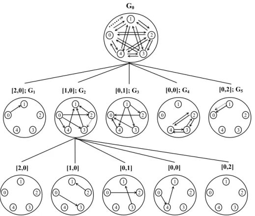
First, we introduce the graphic model by means of a 2×5 AB game for simplicity. We start with some definitions. The game tree for the 2×5 AB game is shown in Fig. 2.1. Any moment in the game is expressed by a node, represented by a game graph Gi=<Vi, Ei>, in the game tree. The root G0=<V0, E0> of the game tree is a complete directed graph with 5 vertices and 20 edges. We map the game graphs to 2×n AB games as follows:
Vertex: Each vertex in a game graph Gi corresponds to a symbol in the AB game; for example, 0, 1, 2, 3, and 4 are five symbols in the 2×5 AB game. Notice that we use the term
“node” in the game tree and “vertex” in the game graphs.
Edge: Each directed edge in a game graph Gi refers to a possible codeword, so there are 5×4=20 edges in the root G0of the game tree. In the medium stages, the edges in a game graph Gi, i 1, refer to the remaining candidates, i.e., the codewords compatible with responses given so far.
Partition edge: the edge codebreaker chooses to partition the game graph; for instance, the dashed arrow (0,1) shown in G0 of Fig. 2.1 refers to the first guess (0,1) in a 2×5 AB game.
Notice that, according the rules of this game, we can choose arbitrary partition edge e E0 (not necessarily e Ei) in the medium stage, for example, (2,3) can be chosen as the partition edge in G2.
Each class, represented as a node in the game tree, in level 2 refers to one response [A, B]
Fig. 2.1. A partial game tree for 2×5 AB game, where (0, 1) and (2,3) are the partition edges in G0and G2, respectively.
G0 1
0
4
2
3
1 0
4 2
3
[2,0]; G1 [1,0]; G2 [0,1]; G3 [0,0]; G4 [0,2]; G5
1 0
4 2
3 1
0
4 2
3 1
0
4 2
3 1
0
4 2
3
1 0
4 2
3
[2,0] [1,0] [0,1] [0,0] [0,2]
1 0
4 2
3 1
0
4 2
3 1
0
4 2
3 1
0
4 2
3
after guessing (0,1) in the game. The five classes in level 2, i.e., [2,0], [1,0], [0,1], [0,0], and [0,2], partition the set of 20 edges in the complete directed graph G0in the root node. Moreover, only one edge (0,1) remains in G1, which refers to class [2,0]. It means that the edge (0,1) was hit. On the other hand, if there is only one edge in a class, except for the class [2,0], then this edge is said to be identified, and one more guess is required to hit it. For example, there is only one edge (1,0) in G5. We need one more guess (1,0) to finish the AB game.
2.1.2 Principles of Partition
Now we will present how to partition the edges on the graph. Remember that a game graph Gi is a directed graph. If the partition edge is (j, k), then vertex j is called the origin vertex, and vertex k is called the destination vertex. We can partition all the edges in the game graph Giaccording to the following simple rules:
(1) The outgoing edges (j, m) from the origin vertex j and the incoming edges (m, k) to the destination vertex k are classified as [1,0], where m≠k, m≠j.
(2) The outgoing edges (k, m) from the destination vertex k and the incoming edges (m, j) to the origin vertex j are classified as [0,1] , where m≠j, m≠k.
(3) The edges that are not adjacent to the origin and destination vertices are classified as [0,0].
(4) The edge (j, k) that is both an outgoing edge from the origin vertex j and an incoming edge to the destination vertex k is classified as [2,0].
(5) The edge (k, j) that is both an outgoing edge from the destination vertex k and an incoming edge to the origin vertex j is classified as [0,2].
As depicted in Fig. 2.1, at the initial stage, the partition edge (0,1) in G0 partitions the 20 edges into five classes. The outgoing edges from the origin vertex 0, i.e., (0,2), (0,3), and (0,4), and incoming edges to the destination vertex 1, i.e., (2,1), (3,1), and (4,1), are classified into class [1,0], i.e., G2. The edge (0,1) is both an incoming edge to vertex 1 and an outgoing edge from vertex 0, so it is classified into class [2,0], i.e., G1. Similar extensions can be given for the
other classes.
2.1.3 Strategies for the 2×5 AB Game
Now we will describe the goals in this study and show how we can achieve them using the graphic model. By means of the partition rules given above, we can translate the game-guessing process into a sequence of graph partition and tree traversal procedures. Notice that all the leaves in the game tree are “hits nodes”; i.e., one candidate is hit in each of the leaf nodes. Therefore, we can directly apply the results described in Observations 1.1 and 1.2 to obtain the optimal strategy for 2×n AB games. Our goals are, thus, to minimize the height H of the game tree for the worst case and to minimize the external path length L of the game tree in the expected case. The key to achieving these goals is simply to choose the best partition edge to partition the remaining edges at each stage, like playing the real game.
In Lemma 2.1, we show how to calculate the total number of guesses required to hit 2 remaining candidates (or 2 remaining edges) in a class (or a game graph). This lemma can be applied to m×n AB games with arbitrary m, n.
Lemma 2.1. If a game graph that is the root node of a game tree contains only two remaining edges, then the minimum possible values for the external path length L and the height H of the game tree are 3 and 2, respectively.
Proof. Sufficient. We can choose one of the two remaining edges as the partition edge. Then, this edge will be hit, and the other edge will be identified and one more guess is required. Therefore, a possible value for the external path length L of the game tree is 1+2=3, and that for the height H of the game tree is 2.
Necessary. For the situation where two edges remain in a game graph, there are only three possibilities for choosing the partition edge.
Case 1. Choose one of these two remaining edges as the partition edge. As described in the sufficient condition, the external path length L of the game tree is 1+2=3, and the height
H of the game tree is 2.
Case 2. Choose an edge adjacent to at least one of the two remaining edges. The best result of these guesses is able to identify the two remaining edges simultaneously, each of which requires one more guess to be hit. So the external path length L of the game tree is 2+2=4, and the height H of the game tree is 2.
Case 3. Choose an edge that is not adjacent to the two remaining edges. The result of this guess makes no contribution to further guesses since the game graph after the guess is the same as the one before the guess. Thus, we can omit this possibility.
Therefore, to hit 2 remaining edges in a game graph (or a class), the external path length L of the game tree must be at least 3, and the height H of the game tree must be at least 2. In other words, the total number of guesses required to hit the two remaining candidates is at least 3. Hence, the number of guesses in the expected case is 3/2=1.5. In addition, the number of guesses in the
worst case is at least 2. ■
Now we will present a strategy for playing the 2×5 AB game on the graphic model and show how to calculate the external path length L and the height H of the game tree. In this way, we can develop sophisticated strategies for higher dimension games. To demonstrate the variety of strategies, the strategies used in the following examples are not necessarily optimal choice.
Observing the first guess in Fig. 2.1, since G0is a symmetric and complete graph, choosing any edge as the partition edge will obtain the same result. We choose (0,1) as the partition edge. After the first guess, there is only one remaining edge (0,1) in G1 (class [2,0]). Notice that Fig. 2.1 shows only one leaf G1, and the distance from the root G0 to G1 is 1. Therefore, edge (0,1) only requires one guess to be hit. Although the edge (1,0) is also the only edge in G5(class [0,2]), one more guess is required to "hit" the edge (1,0), so it requires 2 guesses. Furthermore, it is easy to show that the game graphs G2 and G3 for classes [1,0] and [0,1] are isomorphic; that is, if we exchange vertex 0 and vertex 1 in the game graph G2for class [1,0], then it will be equivalent to the game graph G for class [0,1]. Intuitively, they have the same number of guesses in both the
worst case and the expected case. Therefore, we will concentrate on classes [1,0] and [0,0]. In the following paragraphs, we describe the general procedures used to calculate the number of guesses for the 2×5 AB game in the worst and expected cases.
In G2of Fig. 2.1, the partition edge (2,3) partitions the remaining six edges into three nonempty classes, [1,0], [0,1], and [0,0], each of which has two remaining edges. By Lemma 2.1, the two remaining edges can be hit in one and two more guesses, respectively. Therefore, the external path length for G2, L2= 2+3+2+3+2+3=15; hence, by Observation 1.2, the expected number of guesses for G2is L2/6=2.5.
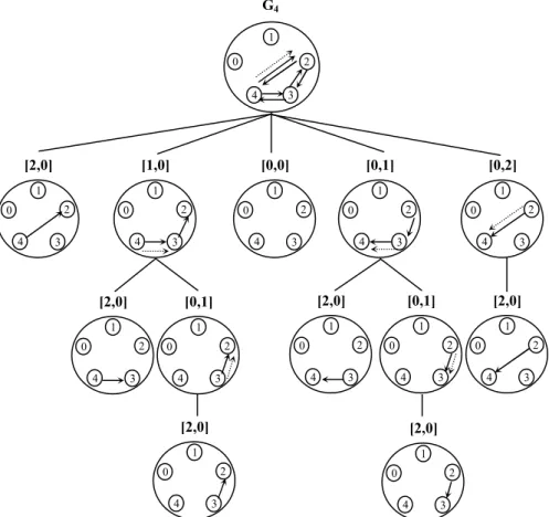
We now consider how to calculate the total number of guesses (or the external path length L4) for the 2×3 AB game in the expected case. In G4shown in Fig. 2.2, there is a complete subgraph with three vertices and six directed edges, which represents the 2×3 AB game. If (4,2) is chosen as the partition edge, as shown in Fig. 2.2, we need 1, 2, 3, 2, 3, and 2 guesses to hit edges (4,2),
1 0
4 2
3
[2,0]
1 0
4 2
3
1 0
4 2
3
[1,0]
1 0
4 2
3
[0,0]
1 0
4 2
3
[0,1]
1 0
4 2
3
[0,2]
1 0
4 2
3
[2,0]
1 0
4 2
3
[2,0]
1 0
4 2
3
[0,1]
1 0
4 2
3
[0,1]
1 0
4 2
3
[2,0]
1 0
4 2
3
[2,0]
1 0
4 2
3
[2,0]
G4
Fig. 2.2. The game tree for G4, which represents the 2×3 AB game.
(4,3), (3,2), (3,4), (2,3), and (2,4), respectively. Therefore, the total number of guesses (or the external path length L4) for the six edges in G4 is L4=1+2+3+2+3+2= 13; thus the expected number of guesses for the game graph G4is L4/6=13/6.
Finally, let us combine Figs. 2.1, and 2.2. If we choose (2,3) and (4,2) as the partition edges in G2 and G4, respectively, then the height of the game tree is 4; that is, by using our analysis technique the number of guesses in the worst case is 4. The total number of guesses L0for G0can be computed as follows: L0= (L1+ L2+ L3+ L4+ L5)+ (the total number of edges in G0) = (L1+1) + (L2+6) + (L3+6) + (L4+6) + (L5+1) = (0+1)+(15+6)+(15+6)+(13+6)+(1+1)=64. Where L1+1 is for G1, L2+6 is for G2, and so on. Therefore, the expected number of guesses for G0=64/20=3.2.
2.2 Optimal Strategies for 2×n AB Games
In this section, the graphic model described in Section 2.1 is used to develop an optimal strategy for 2×n AB games. We first simplify the graph for the games by a recursively graphic representation. Afterward, the optimal strategies for the games in the expected and the worst cases are demonstrated.
2.2.1 Graphic Representation
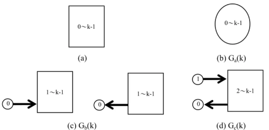
We simplify the graphic representation for the game and define three types of subgraphs, denoted by Ga(k), Gb(k), and Gc(k) in Figs. 2.3(b), 2.3(c), and 2.3(d), respectively. The rectangle shown in Fig. 2.3(a) and the ellipse shown in Fig. 2.3(b), denoted by “i〜j” inside, refer to a graph with only j-i+1 separate vertices named i, i+1, …, j, and a complete directed graph with j-i+1 vertices named i, i+1, …, j, respectively. Notice that the bold arrows in Figs. 2.3(c) and 2.3(d) refer to
“one to all” or “all to one” edges, each of which connects the vertex outside the rectangle to all the vertices inside the rectangle. Hence, there are n-1 and 2(n-2) edges in Figs. 2.3(c) and 2.3(d), respectively.
Definition 2.1. T(k), T1(k), and T2(k) are the minimal external path lengths of the game trees whose roots are the nodes for Ga(k), Gb(k), and Gc(k), respectively. In a similar way, we define H(k), H1(k), and H2(k) as the minimal possible values for the height of the game trees for Ga(k), Gb(k), and Gc(k), respectively.
Lemma 2.2. The minimal number of guesses required for 2×n AB games is T(n)/n(n-1) for the expected case and H(n) for the worst case.
Proof. Since the initial state for 2×n AB games is Ga(n), by Definition 2.1, the minimal external path length and the minimal height of the game tree are T(n) and H(n), respectively. From Observations 1.1 and 1.2, the results of this Lemma follow. ■ 2.2.2 Optimal Strategy in the Expected Case
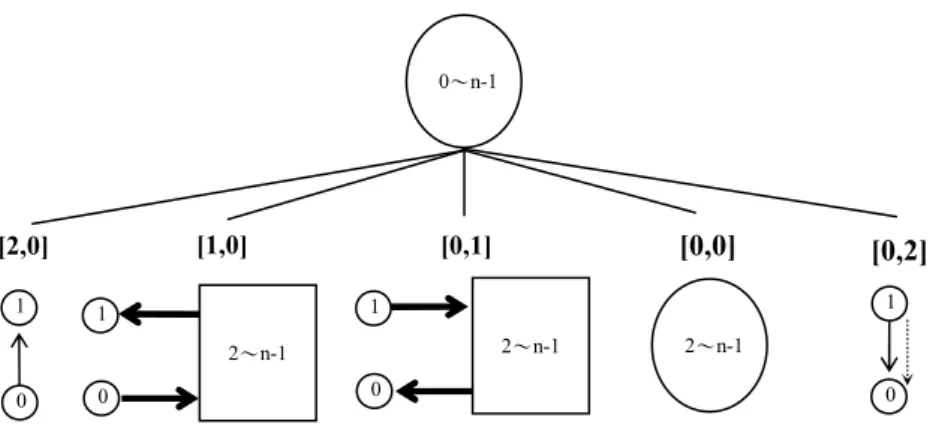
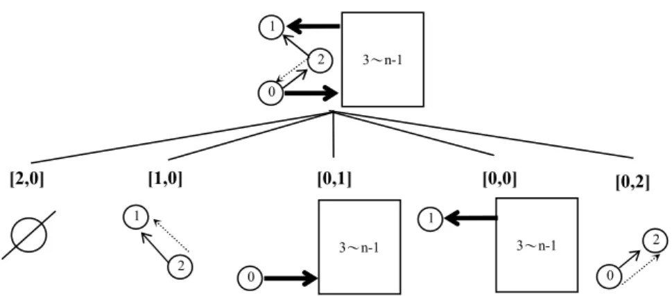
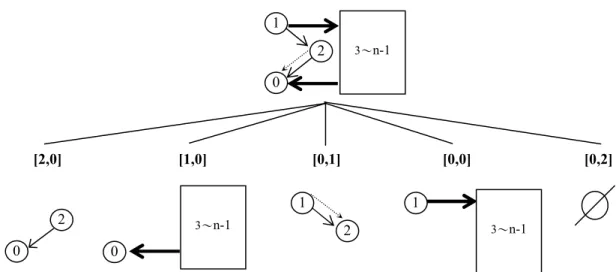
Now we will demonstrate our procedure for deriving T(n) and H(n), by which we can obtain the optimal strategies for 2×n AB games in the expected and worst cases. At the initial state, since the graph Ga(n) is a symmetric and complete graph, we can choose any edge, (0,1) in this example, as the partition edge; consequently, we will obtain the same result. The game tree after the first guess is shown in Fig. 2.4. The minimal numbers of further guesses required for classes [2,0], [1,0], [0,1], [0,0], and [0,2] (the external path lengths of the subtrees whose roots are the
Fig. 2.3. (a) A graph with k vertices and no edges. (b) A complete directed graph, Ga(k), with k vertices and k(k-1) edges. (c) Two types of graphs, Gb(k)s, with k-1 edges. (d) A graph, Gc(k), with 2(k-2) edges.
(d) Gc(k) (b) Ga(k)
0〜k-1
0 1
2〜k-1
(c) Gb(k) (a)
0〜k-1
0
1〜k-1
0
1〜k-1
nodes for classes [2,0], [1,0], [0,1], [0,0], and [0,2]) are 0, T2(n), T2(n), T(n-2), and 1, respectively. In addition, since the number of guesses for each remaining candidate (the length from root to each leaf) will be increased by one after the first guess, we have to add n(n-1) to compute T(n), where n(n-1) is the number of edges before the guess(i.e., in the root node). Hence, T(n) = 0+ T2(n)+ T2(n)+ T(n-2) +1+n(n-1) = T(n-2)+2T2(n)+ n2-n+1.
In Fig. 2.4, since the game graphs for classes [1,0] and [0,1] are isomorphic, and since the game graph for class [0,0] can be solved recursively, we only consider the class [1,0]. The four possible ways to partition the class [1,0], i.e., Gc(n), and their recurrences are described as follows:
1. Choose (0, y) or (y, 1) as the partition edge, where y {2, 3, 4, …, n-1}. The game tree after Fig. 2.4. The game tree for 2×n AB games, where (0,1) is chosen as the partition
edge. T(n)=0+ T2(n)+ T2(n)+T(n-2)+1+n(n-1)= T(n-2) + 2T2(n)+ n(n-1) +1.
[2,0] [1,0] [0,1] [0,0] [0,2]
2〜n-1 0〜n-1
0 1
2〜n-1 0 1
2〜n-1
0 1
0 1
Fig. 2.5. The game tree for graph Gc(n), where (0,2) is chosen as the partition edge.
The notation “ ” in class [0,2] refers to an empty set.
T2(n) 0+T1(n-2)+1+T1(n-2)+2(n-2) = 2 T1(n-2)+2n-3.
[2,0] [1,0] [0,1] [0,0] [0,2]
0 1
3〜n-1 2
2 1
0
2 1
3〜n-1 0
3〜n-1
Fig. 2.6. The game tree for graph Gc(n), where (2,0) is chosen as the partition edge. T2(n) 0+1+T1(n-2) +T1(n-2) +1+2(n-2)=2 T1(n-2)+2n-2.
[2,0] [1,0] [0,1] [0,0] [0,2]
2 1
0 2 0
1
3〜n-1 2
1
3〜n-1 0
3〜n-1
Fig. 2.8. The game tree for graph Gc(n), where (0,1) is chosen as the partition edge. T2(n) T2(n)+2(n-2)= T2(n)+2n-4.
[2,0] [1,0] [0,1] [0,0] [0,2]
0 1
2〜n-1
1
0
2〜n-1
Fig. 2.7. The game tree for graph Gc(n), where (2,3) is chosen as the partition edge. T2(n) 3+3+ T2(n-2)+2(n-2)= T2(n-2)+2n+2.
[2,0] [1,0] [0,1] [0,0] [0,2]
4〜n-1
1
4〜n-1 0
0 1 2
3
0 2 1
0 3 1 2
3
the first guess is shown in Fig. 2.5, where we choose (0,2) as the partition edge. Now, the numbers of further guesses required for the classes [2,0], [1,0], [0,1], and [0,0] are 0, T1(n-2), 1, and T1(n-2), respectively. In addition, we have to add 2(n-2) to compute T2(n), where 2(n-2) is the number of edges before the guess (0,2). Therefore, T2(n) 0 + T1(n-2)+ 1+T1(n-2) +2(n-2) = 2 T1(n-2)+ 2n- 3.
2. Choose (y, 0) or (1, y) as the partition edge, where y {2, 3, 4, …, n-1}. For example, in Fig.
2.6, we choose (2,0) as the partition edge. The numbers of further guesses required for the classes [2,0], [1,0], [0,1], [0,0], and [0,2] are 0, 1, T1(n-2), T1(n-2), and 1, respectively.
Therefore, T2(n) 1+ T1(n-2) +T1(n-2) +1 +2(n-2)=2 T1(n-2)+ 2n-2. Choosing (1,2) as the partition edge will lead to the same result according to similar analysis, so we omit it here.
3. Choose (y1, y2) as the partition edge, where y1, y2 {2, 3, 4, …, n-1} and y1≠y2. For example, in Fig. 2.7, we choose (2,3) as the partition edge. Now, T2(n) 3+3+T2(n-2)+2(n-2) = T2(n-2) +2n +2.
4. Choose (0,1) or (1,0) as the partition edge. As shown in Fig. 2.8, if we choose (0,1) as the partition edge, then there is only one nonempty class [1,0], which contains all 2(n-2) edges;
similarly, if (1,0) is chosen, the only nonempty class is [0,1]. That is, we cannot derive further partition from this guess and also have to add 2(n-2) to compute T2(n). Therefore, T2(n) T2(n)+ 2(n-2).
Observing the above recurrences, the total number of guesses for strategy 2 is always one more than that for strategy 1. In addition, we cannot derive further partition by using strategy 4.
Therefore, we can ignore strategies 2 and 4 here. Now, we can simply investigate strategies 1 and 3 to determine which one is the better. That is, we can determine the optimal strategy for T2(n) = Min(2T1(n-2)+2n-3, T2(n-2)+2n+2 ).
Now we will focus on the graph Gb(n). There are two types of graphs, between which only the edge direction is different, as shown in Fig. 2.3(c). Hence, we can obtain the same numbers of further guesses for these two types of graphs by changing the direction of the partition edge.
Therefore, without loss of generality, we only need to consider one type of graph. Now we will describe the three possible ways to partition Gb(n) and their recurrences as follows:
(i) Choose (0, y) as the partition edge, where y {1, 2, 3, …, n-1}. In Fig. 2.9(a), we choose (0, 1) as the partition edge, which partitions the graph Gb(n) into two nonempty classes, [2, 0] and [1, 0]. The numbers of further guesses for these two classes are 0 and T1(n-1), respectively. In addition, there are n-1 edges in the graph Gb(n). Therefore, T1(n) 0+ T1(n-1)+n-1= T1(n-1) +n-1.
(ii) Choose (y, 0) as the partition edge, where y {1, 2, 3, …, n-1}. We choose (1,0) as the partition edge, which partition the graph Gb(n) into two nonempty classes, [0, 2] and [0, 1].
The numbers of further guesses for these two classes are 1 and T1(n-1), respectively.
Therefore, T1(n) 1+ T1(n-1)+n-1= T1(n-1) +n.
(iii) Choose (y1, y2) as the partition edge, where y1, y2 {1, 2, 3, …, n-1} and y1≠y2. For example, we choose edge (1, 2) as the partition edge, as shown in Fig. 2.9(b). Now, T1(n) 1+ T1(n-2) +1+n-1= T1(n-2)+n+1.
Form the above analysis, we have T1(n)=Min(T1(n-2)+n+1,T1(n-1)+n,T1(n-1)+n-1) = Min (T1(n-2)+n+1, T1(n-1)+n-1).
Fig. 2.9. (a) Strategy (i), where (0,1) is the partition edge. T1(n) 0+T1(n-1)+n-1.
(b) Strategy (iii), where (1,2) is the partition edge. T1(n) 1+ T1(n-2)+1+n-1.
[1,0] [0,0] [0,1]
[2,0] [1,0]
(a) (b)
0
2〜n-1
0
3〜n-1 0
1
2〜n-1 0
1
0 1 3〜n-1
0 2 1
0 2
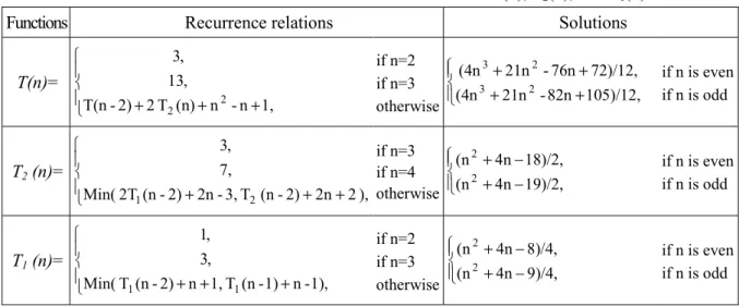
Table 2.1. The recurrence relations and their solutions for T(n), T2(n), and T1(n).
Functions Recurrence relations Solutions
T(n)=
+ +
+2T (n) n -n 1, 2)
- T(n
, 13
, 3
2 2
if n=2 if n=3
otherwise + +
+ +
105)/12, 82n
- 21n (4n
72)/12, 76n
- 21n (4n
2 3
2
3 if n is even
if n is odd
T2(n)=
+ +
+2n-3,T (n-2) 2n 2), 2)
- (n 2T Min(
, 7
, 3
2 1
if n=3 if n=4
otherwise + +
19)/2, 4n (n
18)/2, 4n (n
2
2 if n is even
if n is odd
T1(n)=
+ +
+n 1,T(n-1) n-1), 2)
- (n T Min(
, 3
, 1
1 1
if n=2 if n=3
otherwise + +
9)/4, 4n (n
8)/4, 4n (n
2
2 if n is even
if n is odd
To minimize the total number of guesses, we list the recurrences developed above and their solutions in Table 2.1. Theorem 2.1 demonstrates the minimum number of guesses required for 2×n AB games in the expected case.
Theorem 2.1. The minimum number of guesses required for 2×n AB games in the expected case is (4n3+21n2-76n+72)/12n(n-1) if n is even, and it is (4n3+21n2-82n+105)/12 n(n-1) if n is odd.
Proof. By induction, the recurrences T(n), T2(n), and T1(n) listed in Table 2.1 can be solved as collapsing sums, whose detailed proofs are shown in Appendix A. ■ 2.2.3 Optimal Strategy in the Worst Case
To determine the number of guesses for 2×n AB games in the worst case, we consider the height instead of the external path length of the game tree. We can obtain the recurrences for H(n), H1(n), and H2(n) by slightly modifying the recurrences T(n), T1(n), and T2(n) shown in Table 2.1.
Observing Fig. 2.4, the height of the game tree will be 1 plus the height of the highest among the five subtrees whose roots are the nodes for the five classes. Therefore, we have H(n)=Max(0, H2(n), H2(n), H(n-2), 1)+1= Max(H2(n), H(n-2))+1. We can also obtain this recurrence from the recurrence T(n) = T(n-2) + 2T2(n) +n2-n+1. That is, we can change coefficient 2 associated with the recurrence function T2(n) to 1, the cost (n2-n+1) for each iteration into 1, and the sum operations between the recurrence functions in the right side to Max function. The recurrences
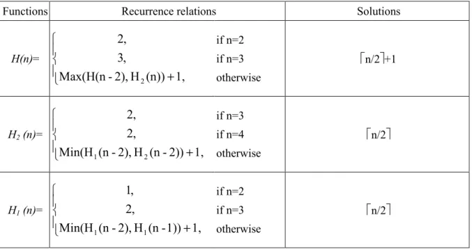
H1(n) and H2(n) can be obtained in a similar way. The recurrence relations and their solutions for H(n), H1(n), and H2(n) are shown in the Table 2.2. Theorem 2.2 demonstrates the minimum number of guesses required for 2×n AB games in the worst case.
Table 2.2. The recurrence relations and their minimum solutions for H(n), H2(n), and H1(n).
Theorem 2.2. n/2 +1 guesses are necessary and sufficient for 2×n AB games in the worst case.
Proof. By induction, the recurrences H(n), H1(n), and H2(n) listed in Table 2.2 can be solved as collapsing sums, whose detailed proofs are shown in Appendix A. ■
We apply the optimum strategy obtained in this section to the 2×5 AB game. The height of the game tree for the strategy used in Section 2.1 for the 2×5 AB game is 4, which has already achieved the best result, H(n) = n/2 +1= 5/2 +1= 4, in Theorem 2.2. Nevertheless, the strategy achieved in G2 of Fig. 2.1, i.e., choosing (2,3) as the partition edge, is not the best choice if we consider the external path length. As proven in Theorem 2.1, if we use the best strategy, i.e., choosing (0, y) or (y, 1) as the partition edge, where y {2, 3, 4}, then the external path length L2
of the game tree will be 13 instead of 15. Thus, the total number of guesses required for the 2×5 AB game is L0=(L1+ L2+ L3+ L4+ L5)+ (the total number of edge in G0)= (0+13+13+13+1) +20
=60. Therefore, the minimum number of guesses required for G0=60/20=3, which achieves the Functions Recurrence relations Solutions
H(n)=
+1, (n)) H 2), - Max(H(n
, 3
, 2
2
if n=2 if n=3 otherwise
n/2 +1
H2(n)=
+1, 2)) - (n H 2), - (n Min(H
, 2
, 2
2 1
if n=3 if n=4 otherwise
n/2
H1(n)=
+1, 1)) - (n H 2), - (n Min(H
, 2
, 1
1 1
if n=2 if n=3 otherwise
n/2
result, (4n3+21n2-82n+105) / 12n(n-1) = (4*53+21*52-82*5+105)/(12*5*4) = 3, in Theorem 2.1.
2.3 Optimal Strategies for 2×n Mastermind Games
In this section, we consider optimal strategies for 2×n Mastermind games. The difference between AB games and Mastermind games is that repetition of colors is allowed in Mastermind games, whereas repetition of symbols (colors) is prohibited in AB games. In Section 2.2, we have used a similar but simpler graphic model to completely solve the 2×n AB games. However, due to the difference between AB game and Mastermind game, the graphic representation for Mastermind games contains self-cycle edges to each vertex. This property introduces lots of analytical difficulties and complexities. That is, much more possible guessing strategies and recursive patterns have to be analyzed and discovered for 2×n Mastermind games. Therefore, the graphic model and optimal strategy for 2×n Mastermind games are more complicated than that for 2×n AB games.
2.3.1 Graphic Representation
To develop an optimum strategy for 2×n Mastermind games, we simplify the graphic representation and define six functions for 2×n Mastermind games as shown in Fig.2.10. The rectangle shown in Fig. 2.10(a), denoted by “i〜j” inside, refers to a graph with only j-i+1 separate vertices named i, i+1, …, j, and without any edge. On the other hand, the ellipse shown in Fig. 2.10(b) refers to a complete directed graph with j-i+1 vertices named i, i+1, …, j. Let T(n), T2(n), T1(n), T12(n), T10(n), and T20(n) denote the minimal external path lengths (the minimal number of guesses required to hit all the candidates) for the six types of game graphs with n vertices, as shown in Figs. 2.10(b), 2.10(c), 2.10(d), 2.10(e), 2.10(f), and 2.10(g), respectively.
Notice that the bold arrows in these Figures refer to “one to all” or “all to one” edges, each of which connects the vertex outside the rectangle to all the vertices inside the rectangle. Hence there are n2, 2(n-2), n-1, 2(n-1), n, and 2(n-1) edges in Figs. 2.10(b), 2.10(c), 2.10(d), 2.10(e),
2.10(f), and 2.10(g), respectively. The subscript for T notation is just used as a symbol to depict the framework of the corresponding graph, as described as follows: T2(n) depicts two vertices outside the rectangle. Tij(n) indicates that i vertices are outside the rectangle, and each of the outside vertices contains a self-circle edge if j=”0”, and the outside vertex is bidirectionally connected to all other vertices within the rectangle if j=”2”. For example, T20 depicts that each of the two outside vertices contains a self-cycle edge, and T12 depicts that there is one vertex outside the rectangle and it is bidirectionally connected to all other vertices within the rectangle.
2.3.2 Optimal Strategy in the Expected Case
Now we will demonstrate our procedure for minimizing the external path length L and the height H of the game tree for 2×n Mastermind games, by means of which we can obtain the minimum number of guesses in the expected and worst cases. Since the initial game graph is symmetric and complete, there are only two possibilities to choose partition edges at the initial stage, (0,1) Fig. 2.10. (a) A graph with n vertices and no edges. (b) A complete directed graph with n vertices and
n2edges. T(n) is the total number of guesses. (c) A graph with 2(n-2) edges. (d) Two types of graph with n-1 edges. T1(n) is the total number of guesses. (e) A graph with 2(n-1) edges. (f) A graph with n edges. (g) A graph with 2(n-1) edges.
0〜n-1
(b) T(n) (a)
0〜n-1
0 (d) T1(n)
1〜n-1
1
0
(c) T2(n) 2〜n-1
0
1〜n-1
0 (f) T10(n)
1〜n-1
0
1〜n-1
(e) T12(n)
0
1〜n-1
(g) T20(n) 1
0
2〜n-1
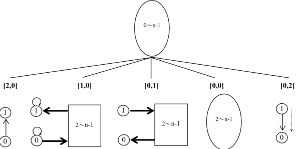
and (0,0). In Fig. 2.11, we choose (0,1) as the partition edge. The numbers of further guesses required for classes [2,0], [1,0], [0,1], [0,0], and [0,2] (the external path lengths of the subtrees whose roots are the nodes for classes [2,0], [1,0], [0,1], [0,0], and [0,2]) are 0, T20(n), T2(n), T(n-2), and 1, respectively. In addition, since the number of guesses for each remaining candidate (the length from root to each leaf) will increase by one after the first guess, we have to add the quantity n2to compute T(n), where n2is the number of edges in the root node. Hence, the minimal number of guesses (the minimal external path length of the game tree) T(n) 0+
T20(n)+ T2(n)+ T(n-2) +1+ n2= T(n-2)+ T20(n)+ T2(n) + n2+1. Likewise, if we choose (0,0) as the partition edge, then T(n) T(n-1)+ T12(n)+ n2. Notice that we use inequality to compute T(n) because T(n) is the minimal value of results derived from 2 cases, (0,0) and (0,1) as the partition edge, in this example.
In Fig. 2.11, since the game graph for class [0,0] can be solved recursively, we only consider classes [1,0] and [0,1]. We first analyze the 6 ways to partition the class [0,1] and then derive the recurrence for T2(n) as follows:
1. Choose (y, 0) or (1, y) as the partition edge, where y {2, 3, 4, …, n-1}. The game graph after this guess is shown in Fig. 2.12, where (2,0) is chosen as the partition edge. Now, The
0〜n-1
Figure 2.11. The game tree for 2×n Mastermind games, where (0,1) is chosen as the partition edge. T(n) 0+ T20(n)+ T2(n)+T(n-2)+1+n2= T(n-2) + T2(n)+ T20(n) +n2+1.
2〜n-1
0 1
0 1
2〜n-1 0
1
2〜n-1
0 1
[2,0] [1,0] [0,1] [0,0] [0,2]
numbers of further guesses required for classes [2,0], [1,0], [0,1], [0,0], and [0,2] are 0, T1(n-2), 1, T1(n-2), and 0, respectively. In addition, we have to add the quantity 2(n-2) to compute T2(n), where 2(n-2) is the number of edges before the guess (0,2). Therefore, T2(n) 0 + T1(n-2)+ 1+T1(n-2) +0 +2(n-2) = 2 T1(n-2)+ 2n- 3.
2. Choose (0, y) or (y, 1) as the partition edge, where y {2, 3, 4, …, n-1}. For example, we choose (0,2) as the partition edge. The numbers of further guesses required for the classes [2,0], [1,0], [0,1], [0,0], and [0,2] are 0, 1, T1(n-2), T1(n-2), and 1, respectively. Therefore, T2(n) 1+
T1(n-2) +T1(n-2) +1 +2(n-2)=2 T1(n-2)+ 2n-2. Choosing (2, 1) as the partition edge will lead to the same result according to a similar analysis, so we omit it here.
3. Choose (y1, y2) as the partition edge, where y1, y2 {2, 3, 4, …, n-1} and y1≠y2. For example, we choose (2,3) as the partition edge. Now, T2(n) 3+3+T2(n-2)+2(n-2) = T2(n-2)+2n +2.
4. Choose (1,0) or (0,1) as the partition edge. If we choose (1,0) as the partition edge, there is only nonempty class [1,0], which contains all 2(n-2) edges; similarly, if (0,1) is chosen, then the only nonempty class is [0,1]. That is, we cannot derive further partition from this guess and also have to add the quantity 2(n-2) to compute T2(n). Therefore, T2(n) T2(n)+ 2(n-2).
5. Choose (0,0) or (1,1) as the partition edge. There are only two nonempty classes, [1,0] and [0,0], for both of which the number of further guesses required is T1(n-1). Therefore, T2(n) 2T1(n-1)+2(n-2).
6. Choose (y, y) as the partition edge, where y {2, 3, 4, …, n-1}. T2(n) 0+3 +0 +T2(n-1) +2(n-2)= T2(n-1)+2n-1.
Observing the above recurrences, the total number of guesses for strategy 2 is always one more than that for strategy 1. In addition, we cannot derive further partition by using strategy 4.
Therefore, we can ignore strategy 2 and strategy 4 here. Now, we can just investigate which is the best of strategies 1, 3, 5, and 6. That is, we can determine the optimal strategy for T2(n) = Min(2T1(n-2)+2n-3, T2(n-2)+2n+2, 2T1(n-1)+2(n-2), T2(n-1)+2n-1).
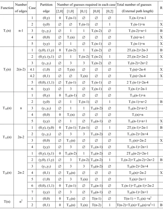
In a similar way, we can obtain all cases of recurrence relations for T(n), T (n), T (n), T (n),
T10(n), and T20(n), as summarized in Table 2.3. The X mark in column R refers that the number of further guesses required is always more than other cases or that it cannot derive further partition, by using the strategy. Moreover, the B mark means that the case would be the best among all strategies, which we will prove in the following paragraphs.
To minimize the total number of guesses, we list the recurrences developed above and their solutions in Table 2.4, whose proofs are shown in Theorem 2.3.
Theorem 2.3. The minimum number of guesses required for 2×n Mastermind games in the expected case is (8n3+51n2 -74n+48)/24n2if n is even, and it is (8n3+51n2-80n+69)/24n2 if n is odd, where n 4.
Proof. By induction, the recurrences listed in Table 2.4 can be solved as collapsing sums, whose
detailed proofs are shown in Appendix A. ■
Fig. 2.12. The game tree for graph T2(n), where we choose (0,2) as the partition edge. The notation “ ” in the class [0,2] refers to an empty set. T2(n) 0+T1(n-2)+1+T1(n-2)+2(n-2)=2 T1(n-2)+2n-3.
0
3〜n-1 1
0
2 3〜n-1
1
3〜n-1 0
2 1
2
[2,0] [1,0] [0,1] [0,0] [0,2]
Table 2.3. The recurrence relations for all strategies for T1(n), T2(n), T10(n), T12(n), T20(n), and T(n).
Number of guesses required in each case Function Number
of edges Case Partition
edge [2,0] [1,0] [0,1] [0,0] [0,2]
Total number of guesses (External path length) R
1 (0,y) 0 T1(n-1) T1(n-1)+n-1
2 (y,0) T1(n-1) 1 T1(n-1)+n X
3 (y1,y2) 1 1 T1(n-2) T1(n-2)+n+1 B
4 (0,0) T1(n) T1(n)+n-1 X
T1(n) n-1
5 (y,y) 1 T1(n-1) T1(n-1)+n X
1 (y,0), (1,y) 0 T1(n-2) 1 T1(n-2) 2T1(n-2)+2n-3 B 2 (0,y), (y,1) 1 T1(n-2) T1(n-2) 1 2T1(n-2)+2n-2 X
3 (y1,y2) 3 3 T2(n-2) T2(n-2)+2n+2
4.1 (1,0) T2(n) T2(n)+2n-4 X
4.2 (0,1) T2(n) T2(n)+2n-4 X
5 (0,0), (1,1) T1(n-1) T1(n-1) 2 T1(n-1)+2n-4 T2(n) 2(n-2)
6 (y,y) 3 T2(n-1) T2(n-1)+2n-1
1 (0,y) 0 T10(n-1) T10(n-1)+n
2 (y,0) 1 T1(n-1) 1 T1(n-1)+n+2 B
3 (y1,y2) 1 1 T10(n-2) T10(n-2)+n+2
4 (0,0) 0 T1(n) T1(n)+n
T10(n) n
5 (y,y) 1 T10(n-1) T10(n-1)+n+1 X
1 (0,y), (y,0) 0 T1(n-1) T1(n-1) 1 2T1(n-1)+2n-1 B
2 (y1,y2) 3 3 T12(n-2) T12(n-2)+2n+4
3 (0,0) T12(n) T12(n)+2n-2 X
T12(n) 2n-2
4 (y,y) 3 T12(n-1) T12(n-1)+2n+1
1 (0,y), (y,1) 0 T10(n-2) 1 T10(n-2) 2T10(n-2)+2n-1
2 (y,0), (1,y) 3 T1(n-2) T10(n-2) 1 T1(n-2)+T10(n-2)+2n+2 B
3 (y1,y2) 3 3 T20(n-2) T20(n-2)+2n+4
4 (0,1) T20(n) T20(n)+2n-2 X
5 (1,0) 3 T2(n) T2(n)+2n+1
6 (0,0), (1,1) 0 T1(n-1) T10(n-1) T1(n-1)+T10(n-1)+2n-2 T20(n) 2n-2
7 (y,y) 3 T20(n-1) T20(n-1)+2n+1
1 (0,0) 0 T12(n) T(n-1) T(n-1) + T12(n) +n2 T(n) n2
2 (0,1) 0 T20(n) T2(n) T(n-2) 1 T(n-2)+T2(n)+T20(n)+n2+1 B
Table 2.4. The recurrence relations and their solutions for T1(n), T2(n), T10(n), T12(n), T20(n), and T(n).
Function and its recurrence relations Solutions
1, if n=2
3, if n=3
T1(n)=
Min( T1(n-1)+n-1, T1(n-2)+n+1 ), otherwise + +
9)/4, 4n (n
8)/4, 4n (n
2
2 if n is even if n is odd
3, if n=3
7, if n=4
T2(n)=
Min
+ +
+ +
+
1 n 2 ) 1 n ( T
, 4 n 2 ) 1 n ( T 2
, 2 n 2 ) 2 n ( T
, 3 n 2 ) 2 n ( T 2
2 1 2
1
, otherwise + +
19)/2, 4n (n
18)/2, 4n (n
2
2 if n is even if n is odd
3, if n=2
6, if n=3
T10 (n)=
Min
+ + +
+ +
+
n ) n ( T
, 2 n ) 2 n ( T
, 2 n ) 1 n ( T
, n ) 1 n ( T
1 10
1 10
, otherwise + +
3)/4, 6n (n
4)/4, 6n (n
2
2 if n is even if n is odd
3, if n=2
7, if n=3
T12 (n)=
Min
+ +
+ + +
1 n 2 ) 1 n ( T
, 4 n 2 ) 2 n ( T
, 1 n 2 ) 1 n ( T 2
12 12
1
, otherwise + +
)/2, 3 1 6n (n
)/2, 14 6n (n
2
2 if n is even if n is odd
7, if n=3
13, if n=4
T20 (n)=
Min
+ +
+ +
+ +
+ +
+ + +
+
1 n 2 ) 1 n ( T
, 2 n 2 ) 1 n ( T ) 1 n ( T
, 1 n 2 ) n ( T
, 4 n 2 ) 2 n ( T
, 2 n 2 ) 2 n ( T ) 2 n ( T
, 1 n 2 ) 2 n ( T 2
20 10 1
2 20
1 10
10
, otherwise
(n2+5n-8)/2
8, if n=2
21, if n=3
T(n)=
Min + + + +
+ +
1 n ) n ( T ) n ( T ) 2 n ( T
, n ) n ( T ) 1 n ( T
20 2 2
12 2
, otherwise + + + +
)/24, 9 6 80n - 51n (8n
48)/24, 74n
- 51n (8n
2 3
2
3 if n is even if n is odd
2.3.3 Optimal Strategy in the Worst Case
To determine the number of guesses for 2×n Mastermind games in the worst case, we consider the height instead of the external path length of the game tree. Let H(n), H2(n), H1(n), H12(n), H10(n), and H20(n) denote the minimum height of the game trees for the game graphs shown in Figs. 2.10(b), 2.10(c), 2.10(d), 2.10(e), 2.10(f), and 2.10(g), respectively. We can obtain the recurrences for H(n), H2(n), H1(n), H12(n), H10(n), and H20(n) by slightly modifying the recurrences T(n), T2(n), T1(n), T12(n), T10(n), and T20(n) shown in Table 2.4. Observing Fig. 2.11, the height of the game tree will be 1 plus the height of the highest among the five subtrees whose roots are the nodes for the five classes. Therefore, we have H(n)=Max(0, H20(n), H2(n), H(n-2), 1)+1= Max(H20(n), H2(n), H(n-2))+1. We can also obtain this recurrence from the recurrence T(n)
= T(n-2) + T20 (n) +T2 (n) +n2 +1. That is, we can change the sum operations between the recurrence functions in the right side to Max function and the cost (n2+1) for each iteration to 1.
The other recurrences can be obtained in a similar way. The recurrence relations and their solutions for H(n), H2(n), H1(n), H12(n), H10(n), and H20(n) are shown in the Table 2.5. We show how to obtain the solutions in Theorem 2.4.
Theorem 2.4. n/2 +2 guesses are necessary and sufficient for 2×n Mastermind games in the worst case.
Proof. By induction, the recurrences listed in Table 2.5 can be solved as collapsing sums, whose
detailed proofs are shown in Appendix A. ■
Table 2.5. The recurrence relations and their solutions for H1(n), H2(n), H 10(n), H 12(n), H 20(n), and H(n).
Function and its recurrence relations Solutions
1, if n=2
2, if n=3
H1(n)=
Min( H1(n-1), H1(n-2) )+1 otherwise n/2
2, if n=3
2, if n=4
H2(n)=
Min( H1(n-2), H2(n-2), H1(n-1), H2(n-1) )+1, otherwise n/2
2, if n=2
2, if n=3
H10(n)=
Min(H10(n-1), H1(n-1), H10(n-2), H1(n) )+1 otherwise
n/2 +1
2, if n=2
2, if n=3
H12(n)=
Min( H1(n-1), H12(n-2), H12(n-1))+1 otherwise n/2 +1
2, if n=3
3, if n=4
H20(n)=
Min( H10(n-2),Max(H10(n-2), H1(n-2)),
H20(n-2), H2(n), H20(n-1) )+1 otherwise
n/2 +1
3, if n=2
3, if n=3
H(n)=
Min( Max(H(n-1), H12(n)), Max(H(n-2), H2(n),H20(n)) )+1, otherwise
n/2 +2
Observing Theorems 2.3 and 2.4, the same strategy can be used to find the optimal solutions for the both cases. Besides, the coefficient of the first term of formulas can be worked out by back-of-the-envelope calculations. Intuitively, the best strategy is to guess two new colors each time until we get two pegs. In the worst case, the second peg won’t happen until n/2 guesses so the total number of guesses is n/2+k. In the average case, the second peg shows up 2/3 of the way to n so the average number of guesses is half of 2n/3+k'=n/3+k"; we further solve the recurrences and derive exact formulas for both the worst and expected cases in Theorems 2.3 and 2.4, respectively.
2.4 Recursive State Transition Diagrams (RSTD)
In this section, we introduce a structure to illustrate optimal strategies obtained in this chapter.
Since the number of the states for general 2×n games is infinite, it is impossible to be describe by a “finite state” transition diagram. We define a new transition diagram, called recursive state transition diagram (RSTD), to illustrate the infinite states. We now introduce an abstract model of RSTD, which is a 6-touple RSTD = (Sr, Sn, d0, R, T, C(d)). The definitions of the elements are described as follows:
1. An integer d0, referred to the dimension of the game. For example, d0=5 for the 2×5 game.
2. A finite set of recursive states Sr= {s0(d), s1(d), s2(d), …}, where d Z. A special element of the set Sr, s0(d0), is referred to the initial state.
3. Three nonrecursive states Sn= {rejecting, identifying, hitting}.
4. A finite set of input responses R = {r0, r1, r2, …}.
5. A function T from S×R to S, referred to the transition function, where S=Sr Sn.
6. A constraint, C(d), referred to the feasible condition. For example, the feasible condition for 2×n AB games is d 2.
At first, the diagram starts at its initial state s0(d0). At any instance afterward, the diagram is in one of its states. If any state does not satisfy the feasible condition, then it will go to the rejecting state. Upon the input response, it will go to another state according to the transition function. Finally, it will terminate in the hitting or rejecting states.
The RSTD for 2×n AB games is shown in Fig. 2.13. The diagram contains six states, i.e., s0(d), s1(d), s2(d), identifying, hitting, and rejecting states. s0(d), s1(d), and s2(d) are recursive states, the graphs for which are Ga(d), Gb(d), and Gc(d) as shown in Figs. 2.3(b), 2.3(c), and 2.3(d), respectively. In a recursive state, although the states are different for different parameter d, the graphs in those states will remain the same recursive structure. We show the name of the recursive state and the optimal strategy in upper and lower parts inside each state, respectively. If a secret code was hit or identified, then the RSTD goes to the identifying or hitting states,